A Spatio-Temporal Analysis of Heat Island Intensity Influenced by the Substantial Urban Growth between 1990 and 2020: A Case Study of Al-Ahsa Oasis, Eastern Saudi Arabia

Abstract

Rapid urbanization has recently led to a significant propagation of heat islands. This study aimed to analyze the spatio-temporal variation in urban heat islands (UHIs) at Al-Ahsa Oasis in Saudi Arabia, in addition to exploring the urbanization influence on UHI distribution over the last 30 years. The spatial variability in UHIs was assessed, the key determinant elements were identified, and the forms of distribution were delineated. Change detection, hot spots, and spatial autocorrelation were employed to study UHI distribution and intensity and to identify the clustering and correspondence between heat and urbanization. The results revealed a considerable increase in built-up areas from 17.15% to 45.8% of total land use/cover (LULC) from 1990 to 2020. No significant variations in UHI intensity were observed (10.4 °C in 1990 and 8.7 °C for 2020). However, a remarkable link was found between urbanization and heat, confirmed by hot spot clustering over intense urban complexes, while cold spot clustering was observed over date and palm tree areas, with 99% confidence for both. Lastly, the link between temperature and urbanization was also confirmed through spatial autocorrelation, producing Moran’s indices of 0.41 and 0.45 for 1990 and 2020, respectively, with an overall significance (p-value) of 0.001. The mechanisms applied have proven their robustness in assessing the effect of urbanization on heat island distribution and quantification.

1. Introduction

The variation between a city’s temperature and that of its countryside area generally relies on the geometry of buildings (for example, their shape and orientation, as well as their construction and street size), in addition to particular built-up cover characteristics (i.e., heat, albedo, wetness, etc.) [1]. The geometry and distribution of streets in metropolis areas significantly affect the development of the surface temperature, leading to heat islands. A change in these attributes transforms the balanced radiation, heat capacity, and energy division into latent heat, as well as sensible heat [2]. Substantial amounts of impermeable surfaces within the urban environment are a result of rapid growth, which is actually regarded as an essential contributing element to UHIs. Reducing the quantity of impermeable surfaces within metropolitan areas is essential in order to diminish UHIs and preserve habitats [3].

Elevated temperatures aggravate power requirements within towns and cities, as they necessitate air-cooling to keep properties cool [4]. Additionally, the use of air cooling units throughout both domestic and industrial areas increases the UHI intensity [5]. Consequently, stress on electrical power availability increases on summer afternoons, which is the time of highest demand. The quality of the air, along with greenhouse gas emissions, should also be considered; emissions of greenhouse gases are boosted as a consequence of increasing power demand [6]. Such emissions negatively affect people’s health and can contribute to atmospheric complications, such as acid rain. Additionally, CO₂ released from power plants that are run by fossil fuels contributes to global changes in the climate [7].

Land use transformation brought about by urbanization [8] is the major driving force behind UHIs [9]. A lower albedo, as well as the greater sealing level of urban areas, considerably affect the energy budget at the surface, bringing about greater heat than in non-urban locations [10]. The assessment of urban heat island intensity (UHII) relies on descriptions of pixels that represent urban and/or rural land [11]. Urban areas tend to be significantly impacted by anthropological behaviors, higher variability in impervious cover, and diverse ecosystems present in the adjacent countryside [12]. An understanding of how UHIs may respond, in terms of intensity and distribution, to these human activities was crucial to precisely estimate the imminent UHI effects over the study area. Typical data on these effects are principally significant for oases, as variations in LULC might occur as a reaction to human interventions and climatic changes.

To solve UHI problems, an assessment of UHIs should be conducted, taking into account the spatiotemporal changes between all surface cover aspects. With the aim of quantifying alterations in LULC and UHIs, GIS utilization, along with remote sensing data, have become progressively more essential. Such technologies are usually affordable and enable monitoring of the degree of, and also the spatial and temporal differences in, UHIs [13]. The most popular indices used for estimating the spatiotemporal deviation in land surface temperatures (LSTs) are the “normalized difference vegetation index (NDVI)” and the “normalized difference built-up index (NDBI)”, which can be determined via satellite data [14]. These two indices are usually used as measures of LULC dynamics [15]. Several researchers have explored the interactions between LULC and LST utilizing satellite images and GIS at the local, regional, and even global scales [16]. However, few research works have focused on arid and semiarid urban oases, where intense surface UHIs are predicted. Several studies have investigated and utilized numerous techniques to determine UHIs [13,17,18]. For example, Tran et al. [19] applied spatial information to evaluate the highest surface UHI. Hafner and Kidder [20] employed an approach in order to determine surface UHIs, where they were assessed in certain scientific studies as a comparison of averages, as well as ultimate heat levels, among settled and non-settled areas. Zhou and Chen [21] have documented that a decline in lake features may increase UHI intensity. Others have evaluated heat during certain periods; for instance, on a seasonal, monthly, annual, or daily basis. In some circumstances, UHIs have been determined by measuring heat alterations over time [22]. Furthermore, Magee et al. [23] determined UHIs by measuring the mean transformed heat over both built-up and rural surfaces. Regarding surface UHI assessment, the comparison between average urban and non-urban forms has offered strong results. The development of LSTs in pre- and post-urbanized locations has highlighted the impact of substantial urban growth on heat islands; however, several towns did not have historical information on surface temperature prior to urban growth, making surface UHI assessment difficult [23]. Recent research performed by Maskooni et al. [13] discovered that spatial changes within LULC can lead to changes in LST patterns.

Furthermore, several studies have recently documented the impact of urban development and land use/cover (LULC) changes on land surface temperature, landscape thermal conditions, and urban heat island (UHI) intensity [24,25,26]. For example, built-up areas correlate positively with LST, while vegetation cover correlates negatively with LST [27]. Furthermore, the density of vegetation and impervious cover—its position, randomness, and accumulation—were found to be highly correlated with LST [25]. A subsequent study, conducted in the Atlanta and Minneapolis metropolitan areas in the United States, documented the magnitude and temporal variations of UHIs [26], and they found that UHIs differ substantially between urban and non-urban areas.

However, very few UHI studies within the literature focused on arid areas have been performed. Some investigators have examined the influence of LULC on UHI intensity over the Al-Ahsa Oasis of Saudi Arabia through utilizing both terrestrial data and satellite images [28]. One constraint of the applied method was assessing UHIs in urban areas compared to the surrounding towns, disregarding the bare soils and sands around the city, which are expected to have a substantial LST influence in arid and semi-arid areas. Other work, however, has directly evaluated LST images with no customization [29], which produced results that were lacking scientific rigor since the atmospheric circumstances were not identical during the image acquisition period.

Throughout the literature review, issues and areas for further study were highlighted. For instance, information regarding the spatiotemporal difference of UHIs in the semi-arid environment of the Al-Ahsa area were lacking detail on the particular impact of LULC development on UHIs. Therefore, this study aimed to quantify and analyze the spatiotemporal variation in UHIs in the arid Al-Ahsa region, in addition to exploring the extent to which urban growth during the last 30 years could have affected heat island distribution. The specific objectives were (1) quantifying the spatial variety in the UHIs in a semi-arid climate-based region, (2) assessing the key determinant elements and the spatial and temporal forms of NDBI and surface temperature distribution, and (3) measuring the influence in LULC evolution on land surface temperature over a time period of 30 years. The outcomes will be a significant step forward in understanding how urban development and a decline in green vegetation cover, particularly in arid and semi-arid oases, may affect habitat stability and human activities through the increase of UHI intensity and changes in spatial distribution.

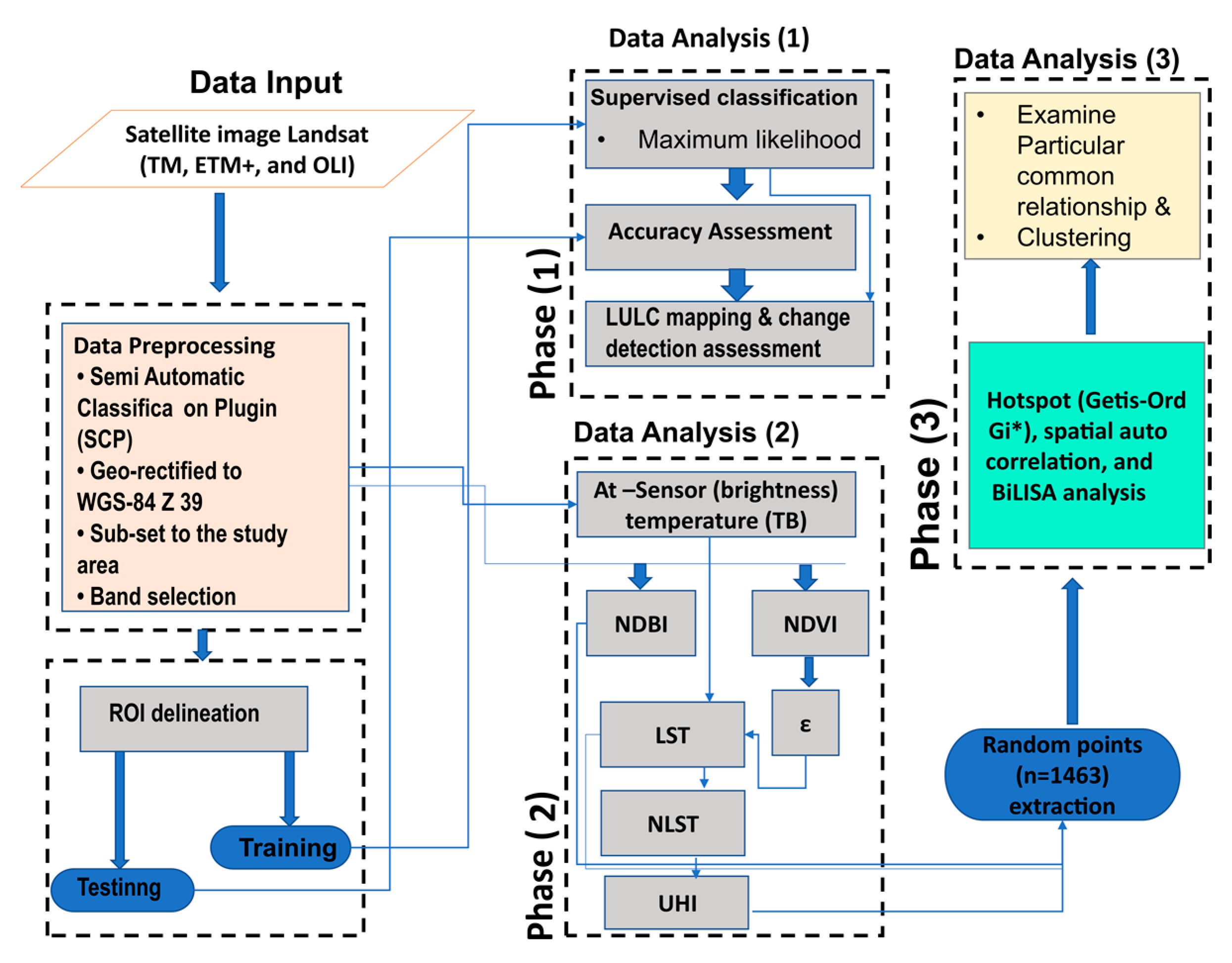
2. Materials and Methods

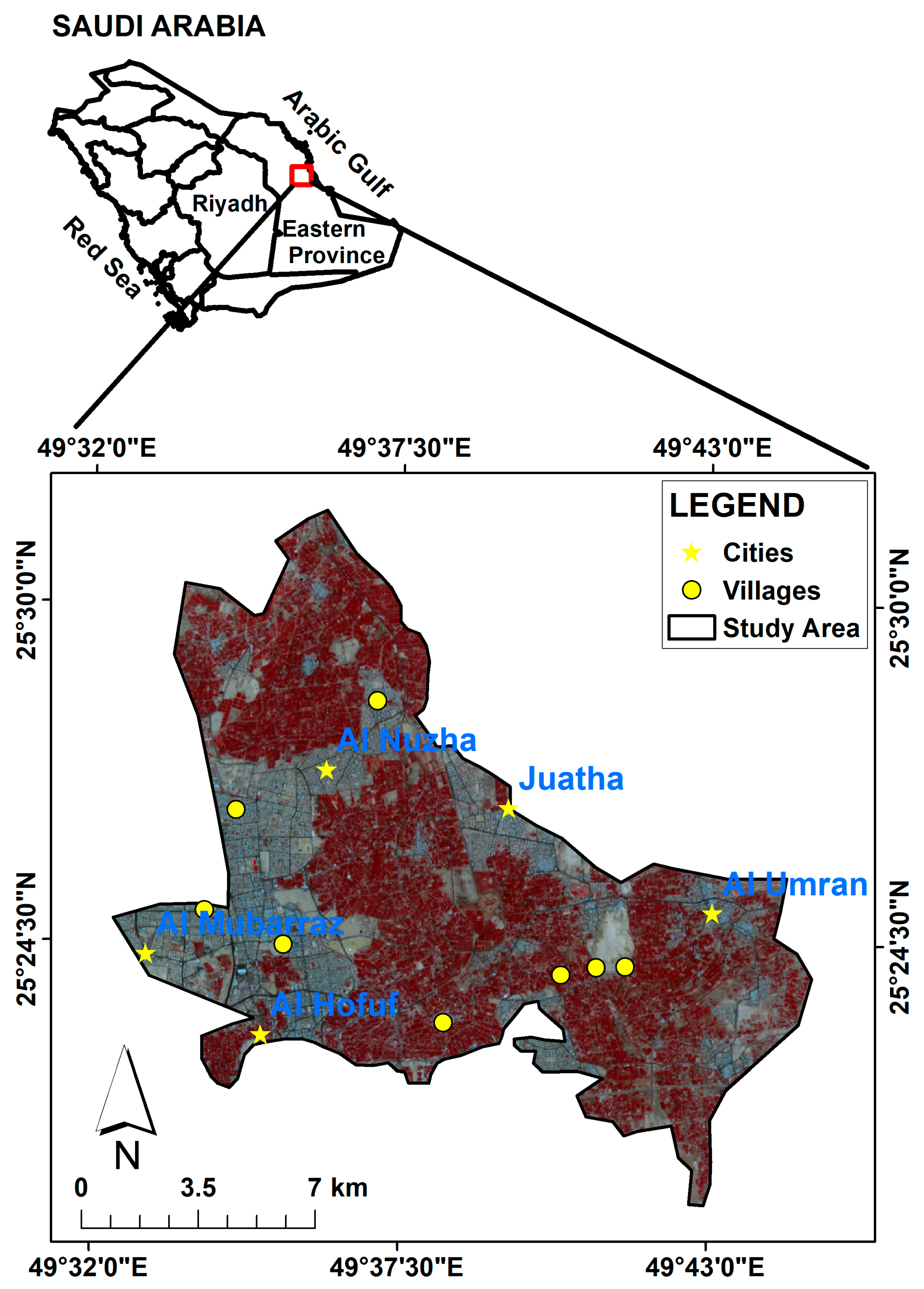
The given flow chart (Figure 1) presents the procedures and steps to build an autocorrelation mechanism to measure and depict the nature of the relationship between the extracted heat islands and the urban impervious surfaces in the study area. As illustrated, the methodology can be summarized in three major steps: (1) preparing data (Landsat images): image acquisition, image preprocessing; (2) extracting features from Landsat imagery using supervised classification and change detection, surface temperature extraction, and heat island assessment and delineation; and, lastly, (3) the execution of the spatial autocorrelation approach.

2.1. Study Area

A pilot study area of 225 km² within the Al-Ahsa Oasis, Kingdom of Saudi Arabia, was selected to carry out the work. The oasis is the biggest agronomic oasis in the kingdom, and possibly the biggest watered oasis in the world [30]. It is situated 45 km inland of the western Arabian Gulf coast and 320 km east of Riyadh, the Kingdom’s capital city. It is located between latitudes 25°20′–25°32′ N, longitudes 49°30′–49°45′ E (Figure 2), and its altitude varies from 160–130 m above MSL from the west to the east. Records from research recently published by Abdelatti et al. [31] revealed that in 1992, the population of the study area was 445,000. It had increased to 768,000 by 2016. In 2017, there were 149,905 houses in the area, representing 24.2% of all houses in the eastern province. Between 1994 and 2014, approximately 66% of the original muddy-structure houses were turned into concrete, 25% into bricks, and 5% into stone [32]. The research region has a very mild topographic surface with minimal relief and few adjoining hills [33]. Energetic and portable sandy hills outline the surface area. Over many centuries, the mobile nature of the sands has caused their encroachment into green cover areas, threatening farmers in the oasis [33]. This growth is handled with actions like dune containment and shrub plantations.

Agricultural activity is a principal livelihood for the citizens of Al-Ahsa, and mostly relies on a water supply from a number of springs in addition to underground sources. Alghannam and Al-Qahtnai [34] documented that the Al-Ahsa Oasis is a crucial agricultural area for the eastern region of the Kingdom. The overall cultivated area is around 8000 ha, of which 92% is designated for date-palm plantations [35]. The soil of the oasis is rich and productive. The water and soil situation in this area motivated authorities to launch a project for irrigation and drainage in 1971, aiming to maintain agricultural activities. This specific cultivated area comprises about 25,000 small farms.

Many studies carried out in the Al-Ahsa Oasis have confirmed the rapid progression of urbanization and its influence on the centralization of UHIs over certain spots, mainly those occupied by built-up surface cover. Investigational research conducted by Elsayed [36], aiming to measure the AL-Ahsa oasis’ vulnerability to urban heat islands, showed that a substantial surge in urban development in Al-Ahsa Governorate took place followed by a temperature increase, confirming that the Al-Ahsa Governorate is susceptible to the occurrence of UHIs. Al-Ali [28] carried out a comparative UHI study over the oasis, making use of LST derived from thermal bands of satellite imagery and field observations of fixed and mobile temperature, as well as relative humidity logging stations, in the summer and winter seasons. The study outcomes revealed a substantial association between the spatial distribution of UHIs and land cover, where the peak intensity of UHIs centered over the two main oasis cities (Al Hufuf and Al Mubarraz). However, neither study considered the nature of the spatial association between LST and built-up area distributions, or the temporal effect that signifies the dynamic nature of UHIs in cities and rural areas.

2.2. Data Types and Preprocessing

The analyses were based on four Landsat images, including Thematic Mapper (TM, Landsat 5), Enhanced Thematic Mapper Plus (ETM+, Landsat 7), and Operational Land Imager and Thermal Infrared Sensor (OLI and TIRS, Landsat 8), recorded in 1990, 2000, 2010, and 2020, respectively (

Table 1. Landsat image characteristics.

Sensor-ID	Spacecraft-ID	Acquired Date	No. of Bands	Spatial Resolution
TM	Landsat-5	15 July 1990	6(reflective), 1(thermal)	30 m (reflective), 120 m (thermal)
ETM+	Landsat-7	2 July 2000 14 July 2010	6 (reflective), 2 (thermal)	30 m (reflective), 120 m (thermal)
OLI and TIRS	Landsat-8	17 July 2020	8 (reflective), 2 (thermal)	30 m (reflective), 100 m (thermal)

). All images were freely obtained from the US Geological Survey (USGS) Earth Explorer website (http://earthexplorar.usgs.gov/ (accessed on 5 February 2022)).

All images were carefully collected during the dry season (July) to reduce the impact of scene variations and illumination conditions. The scenes covered path 164 and row 042, had a spatial resolution of 30 m for optical bands and 60 to 100 m for thermal bands, and were cloud-free. Landsat images were selected because of their availability and their potential to provide reflective and thermal infrared bands that can be used to estimate different elements, including the normalized difference built-up index (NDBI), land use/land cover (LULC), normalized difference vegetation index (INDVI), and land surface temperature (LST).

We geo-rectified the images to the WGS84/UTM, zone 39 N. Radiometric calibration, atmospheric correction, and a gap-filling process were performed for the July 2010 image using data-specific utilities, the dark object subtraction (DOS) technique, and the gap-filling tool, utilizing ENVI 5.1 image processing software. All other images were atmospherically corrected and radiometrically calibrated by employing a Semi-Automatic Classification Plugin (SCP) [37] of the open-source QGIS software program (version 3.16). Images with pixel values ranging from 0 to 1 were obtained from the pre-processing operations; then, a subset covering the pilot area (Figure 1) was delineated and clipped.

2.3. Classification of LULC and Assessing Its Accuracy

Land cover classes, including vegetation cover (mainly date palm plantation trees), built-up cover, bare lands, and sand dunes, were extracted from each individual Landsat image by employing a widely utilized maximum likelihood algorithm, which is a supervised classification method [38]. The (ENVI) version 5.1 software environment was utilized for visualizing and processing the images. The classification process was achieved by creating training samples (spectral signatures) according to Anderson’s classification Level-1 scheme [39], selected visually from the images. A minimum of six or seven training areas containing at least 150 pixels were selected from each LULC class. After this, the image classification was performed and then output maps were evaluated and exported to the ArcGIS 10.2 software program for further operations, which entailed the calculation of areas and thematic layers preparation.

To validate the LULC map accuracy, we used the overall accuracy and kappa coefficient approaches. Initially, 22 validation points were collected randomly from each category. Thus, in total, 87 points were collected and overlaid on the Google Earth software’s base map, where every LULC class was verified by superimposing the Google Earth satellite image, taken on May 2020. Second, a confusion matrix was built to assess the obtained LULC maps. Finally, previous studies have suggested the use of quantity disagreement and allocation disagreement to assess the classification accuracy [40,41]. However, in this study, the overall accuracy, producer accuracy (PA), and use accuracy (UA), in addition to errors of omission and commission, were used as previously described [42] to assess the classification accuracy.

2.4. LULC Change Detection

The post classification comparison method [43] was used to identify changes in LULC that occurred in the study site throughout the study period. This approach was chosen because of its straightforwardness and clarity, and because it is the most commonly quantitative method applied to detect changes in independently obtained LULC maps. Moreover, it does not require image-to-image registration [43]. Challenges may arise when classifying multi-date data, such as the combination of features (mixture) per-pixel and the errors inherent from using two classification maps [44]. In this method, the actual change was obtained by comparing the LULC map from one date to that obtained on another date, resulting in a change matrix.

2.5. Estimation of LST

The satellite’s LST provides crucial data for assessing the influence of urbanization [45]. Landsat satellite thermal band images were utilized to uncover the surface heat’s locative scattering, in addition to measuring the LULC effect on LST within the research region. Concerning the LST calculation, the method used was explained by Guo et al. [46]. The temperature information was acquired by making use of Landsat’s (TM and ETM+) digital number (DN) (0–255) and the Landsat’s OLI (DN 0–65,536) thermal bands. The DN was then transformed to Kelvin temperature in two actions. Initially, the DN value to spectral radiance made use of the next method [47,48]:

$$L_{\lambda }=M_L\times QCal+A_L$$

(1)

$$L_{\lambda }=\frac{L{max}_{\lambda }-L{min}_{\lambda }}{{QCal}_{max}-{QCal}_{min}}\times \left({QCal}_{max}-{QCal}_{min}\right)+Lmi{n}_{\lambda }$$

(2)

In which $L_{\lambda }$ denotes the spectral radiance W/(m² sr μm), $M_L$ is a multiplicative element for scaling the thermal bands’ radiance, QCal represents the digital number, A_L is an additive element for the band radiance scaling, $QCa{l}_{max}=255$, $QCa{l}_{min}=1$, and $Lma{x}_{\lambda }$ and $Lmi{n}_{\lambda }$ denote the thermal bands’ spectral radiance at DN = 255 and 1, respectively (given in W/m² ster μm) [14].

Secondly, thermal infrared information was then developed by extracting the brightness temperature ($T_B$) from the above-calculated spectral radiance. The transformation method can be explained as follows [14,47]:

$$T_B=\frac{K_2}{Ln\left[\frac{K_1}{L_{\lambda }}+1\right]}$$

(3)

where $T_B$ is the $T_B$ (given in °K), and $K_1$ and $K_2$ represent thermal band’s conversion constants. For Landsat 4 (TM), $K_1$ is 607.76 and $K_2$ is 1260.56; for Landsat 7 (ETM+), $K_1$ is 666.09 and $K_2$ is 1282.71; for Landsat 8 (OLI), $K_1$ is 774.89 and $K_2$ is 1321.08. All $K_1$ and $K_2$ values are given in mW/cm²/sr/μm and Kelvin, respectively.

2.6. LST Calculation

With the aim of determining surface temperature, NDVI was computed by using both the red (RED) and the near-infrared (NIR) images band [49]:

$$NDVI=\frac{NIR-RED}{NIR+RED}$$

(4)

In fact, NDVI remained a key quantitative interpreter for the green cover. It varied from −1 to +1, in which the lesser (+) figures suggest built-up or bare ground, and larger (+) estimates suggest flora [50], while (-) estimates indicate non-vegetated surface types or water [50]. Conversely, surface emissivity (ε) was assessed based on Simwanda et al. [51]:

$$\epsilon =m P_V+n$$

(5)

where n = 0.004, m = 0.986, and P_V represents the amount of vegetation [15], and it was given by the following formula:

$$P_V={\left(\frac{NDVI-NDV{I}_{min}}{NDV{I}_{max}+NDV{I}_{min}}\right)}^2$$

(6)

Ultimately, LST in °C was calculated according to Sultana and Satyanarayana [15], making use of the identified NDVI and ε driving forces:

$$LST=\left(\frac{T_B}{1+\left(\lambda \times \frac{T_B}{\rho }\right)Ln \epsilon }\right)-273.15$$

(7)

where λ denotes the radiance’s released wavelength. ρ = h × c/σ (1.438 × 10⁻² m K), h is a constant of Planck which equals 6.626 × 10⁻³⁴ Js, c is the sunlight speed, which equals 2.998 × 10⁸ m/s, and σ is a constant of Boltzmann, which equals 1.38 × 10⁻²³ J/K.

To obtain the changes in LST and LULC, the stage change of a provided pixel timewise was evaluated using a cross-tabulation process by the analysis of gain-and-loss [52].

2.7. NDBI

NDBI is commonly used in the literature [53] to map built-up features and differentiate between urban and non-urban areas. It relies on two spectral bands, NIR and MIR bands. The NDBI was calculated using the following equation [54]:

$$NDBI=\frac{\left(MIR-NIR\right)}{\left(MIR+NIR\right)}$$

(8)

where MIR and NIR are the middle-infrared and near-infrared spectral bands.

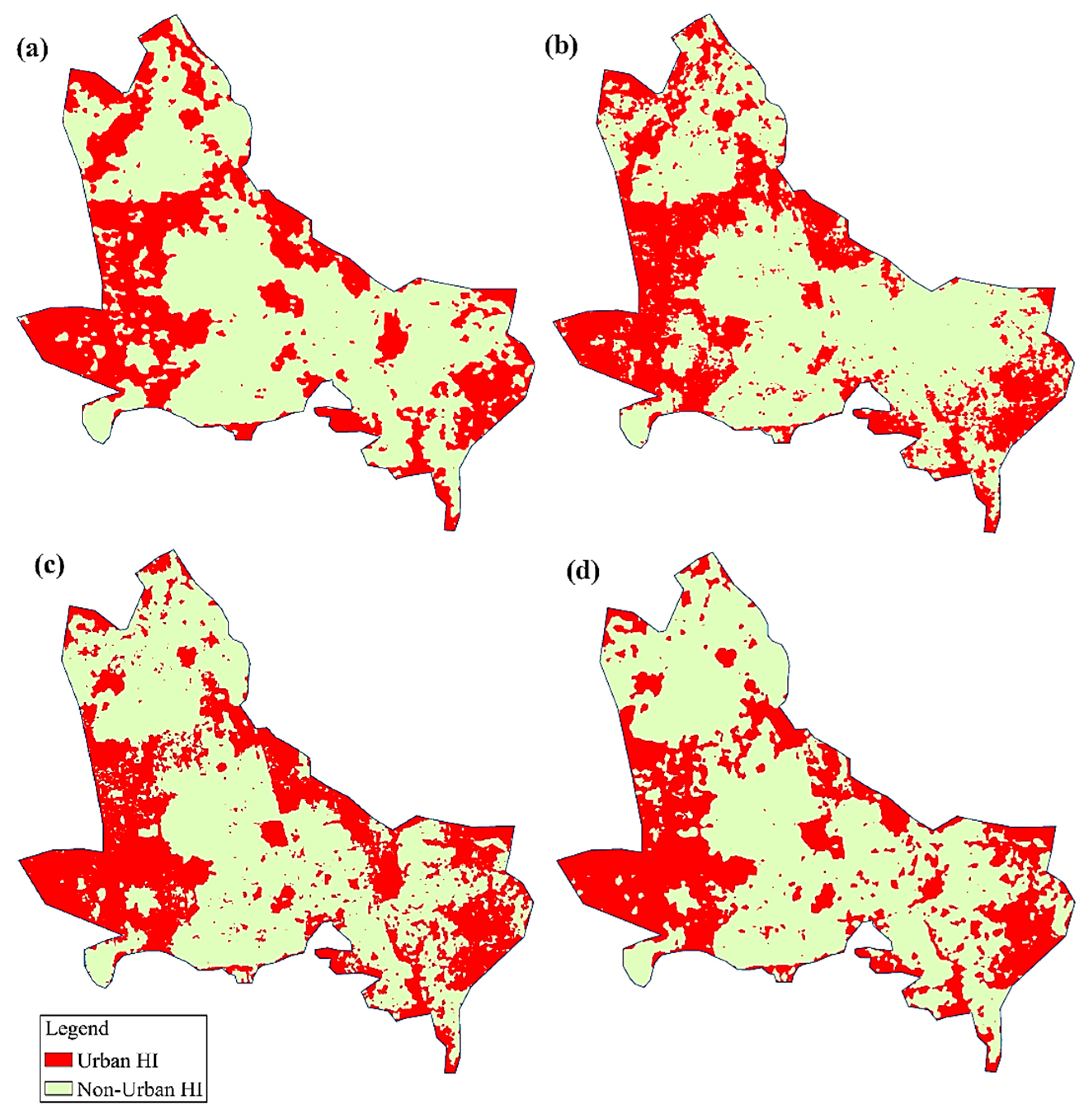
2.8. Mapping UHIs and UHI Intensity and Impact Assessment

UHIs are related to the temperature difference between cities and their adjoining countryside areas [55]. Urbanization and meteorology increase the risk of UHI formation and their effects due to the evolution in urban heat, because of electrical energy demands within urban areas [56]. UHI severity represents the variance among UHI mean temperatures and the mean temperatures of non-urban spots [57]. Landsat data were employed for UHI recognition in this study [58]:

$$UHI Intensity (℃)=T_u-T_r$$

(9)

$$LST>\mu +0.5\times \delta referred to UHI area$$

$$0<LST\le \mu +0.5\times \delta referred to non-UHI area$$

where T_u represents the temperature over the built-up area, T_r represents the non-urban (adjoining) heat, and μ and δ represent temperature average and standard deviation within the location, respectively. The presence of a UHI is denoted by positive values, (i.e., the city heat is greater than the heat of the countryside). In contrast, when urban heat is much less than non-urban heat, negative UHI intensity values are produced, suggesting an urban cool island. The temperatures in Equation (9) could be air, radiant, or surface temperatures. The impact of UHIs is generally estimated according to these temperatures (air, radiant, or surface) so that UHI influences can be specifically determined [59]. Throughout a hot period, for instance in summertime, water bodies in the city, like waterways, pools, and watercourses, might additionally impose cooling influences within the nearby built-up spots. The influence of cooling is brought on via evaporation and the consumption of heat [60].

2.9. Spatial Autocorrelation Analysis

2.9.1. Hot Spots Analysis

Analyzing hot spots remains crucial for uncovering the data trends and patterns and detecting and mapping regions with statistically significant high spatial values clustering (hot spot), as well as low values (cold spot), for both NDBI and LST. The process could be easily achieved using Getis-Ord Gi* statistics [61]. Hence, a hot spot analysis was performed via random points (n = 1463) selected from the NDBI and LST images across the study area by employing the ESRI^® ArcGIS (version 10.2^®) software program. NDBI and LST pixel values corresponding to each point were obtained by using the extraction tools of the software. The output from the analysis was statistically interpreted using the z-score and p-value. A greater z-score plus lower p-value indicated high clustering of features with high values (hot spot), while a smaller (-) z-value plus lower p-value suggested feature clustering with lower values (cold spot). A z-score close to 0 indicated no clustering of either high or low values within the regarded feature [62]. In the current study, NDBI and LST’s hot and cold spots were classified into seven classes based on their Gi* values. Gi* > 0 was regarded as a hot spot with 99%, 95%, and 95% confidence; Gi* < 0 was regarded as a cold spot with 99%, 95%, and 95% confidence; and Gi* = 0 was regarded as “not significant”. The results obtained from these analyses were used to investigate the spatiotemporal patterns of a hot and cold spots with regards to NDBI and LST over the study area. Univariate Local Moran’s I test (p < 0.05) was performed to determine any significant clustering (spatial autocorrelation) for both NDBI and LST over the study area by using GeoDa, an open-source software product [63].

2.9.2. Grid Map Delineation and Class Pixels Extraction

In order to obtain a tight spatial correlation between the heat emitted from buildings (recorded by the thermal bands of satellite images) and the impervious surfaces represented by NDBI, and because the area of study was characterized by a large interference of green cover with built-up surfaces spread beneath it, the area was split into a network of sites (grid), in which each site consisted of a cell with an area of 1 km², within which all data were extracted as single values representing the cell’s spectral properties. The 1 km² sized grid was assumed to represent all possible surface features (urban, date palm trees, bare lands) that were available within the oasis’ metropolis. This was confirmed by direct observation of the city-structure aspects.

The applied grid method used in this study could potentially assist in determining the heat emitted from sole urban surface cover and areas covered with sole vegetation, in addition to the amount of heat emitted by holistic surface covers (urban and vegetation). Hence, it could be used to determine the spatial delineation of the heat islands and relate them to spatial phenomena that have a direct impact on heat island formation and distribution, through applying spatial autocorrelation mechanisms. In addition, by applying spatial gridding, it was possible to study the spatial correspondences between the heat islands and urban complexes without the need for geometric correction of satellite images, which may be complex due to variability in the spatial resolution between the thermal and optical regions in the satellite image’s spectrum.

2.9.3. Application of Spatial Autocorrelation

A spatial autocorrelation approach was carried out to study the existing correspondences between the heat intensity and impervious surfaces, represented by built-up areas. The Bivariate Local Indicator of Spatial Autocorrelation (BiLISA) approach was implemented, aiming to identify any common relationship, bundling, and the importance of the cell-based clustering grid. The BiLISA approach reveals the degree to which the nature of association amongst every pair of variables varies throughout a specific location. Moran’s index (I) was again utilized to evaluate the spatial autocorrelation performance, as well as to measure the spatial reliance within the pair of variables applied [64]. The eventual BiLISA output is usually portrayed in a map, which helps with identifying particular features of the driven autocorrelations, which are usually grouped into four ranks. Two ranks present the affirmative clusters (high with high, and low with low), in agreement with grid cells exactly bordered by other adjacent cells possessing typical values. The contrasting two ranks include outliers (high with low, and low with high), that generally correspond to grid cells whose other bordering cells incorporate diverse values. A GeoDa software program [63] that provides a remarkably accessible environment for spatial autocorrelation data utilization and assessment was used for the analysis.

3. Results

3.1. Classification of LULC and Assessing Its Accuracy

Using the subset of the Landsat-5 (TM), Landsat-7 (ETM), and Landsat-8 (OLI) images, the LULC maps were independently generated by applying the maximum likelihood classification approach. The classified maps are displayed in Figure 3a–d. Throughout the entire study period (1990–2020), the transformation from vegetation cover and bare land to urban was dominant.

The overall accuracy of the final LULC maps extended from 90.2% to 95.9%, and the user’s and producer’s accuracy ranged from 68% to 100% (

Table 2. Accuracy assessment of LULC classification results for the study area from 1990 to 2020.

LULC Class	1990				2000				2010				2020
	UA (%)	PA (%)	OE	CE	UA (%)	PA (%)	OE	CE	UA (%)	PA (%)	OE	CE	UA (%)	PA (%)	OE	CE
Vegetation	100	100	0	0	100	100	0	0	95.12	100	0	4.9	100	100	0	0
Built-up	84.09	100	0	15.9	93.18	100	0	6.8	95.45	95.45	4.5	4.5	93.18	100	0	6.8
Bare land	88.24	68.18	31.8	11.8	94.12	88.89	11.1	5.9	94.12	88.89	0.1	5.9	88.24	93.75	6.3	11.8
Sand dunes	85	77.27	22.7	15	95	86.36	13.6	5	95	90.48	9.5	5	100	83.33	16.7	0
Overall accuracy	90.2%				95.9%				95.1%				95.9%

UA stands for user’s accuracy; PA stands for producer’s accuracy; OE stands for omission errors; and CE stands for commission errors.

). The values of the omission and commission errors ranged from a min. value of 0 for both to max. values of 32 and 15, respectively (Table 2). Generally, these accuracies indicated a significant correlation amongst the LULC maps and the reference points, indicating the reliability of the classification method used and the obtained results.

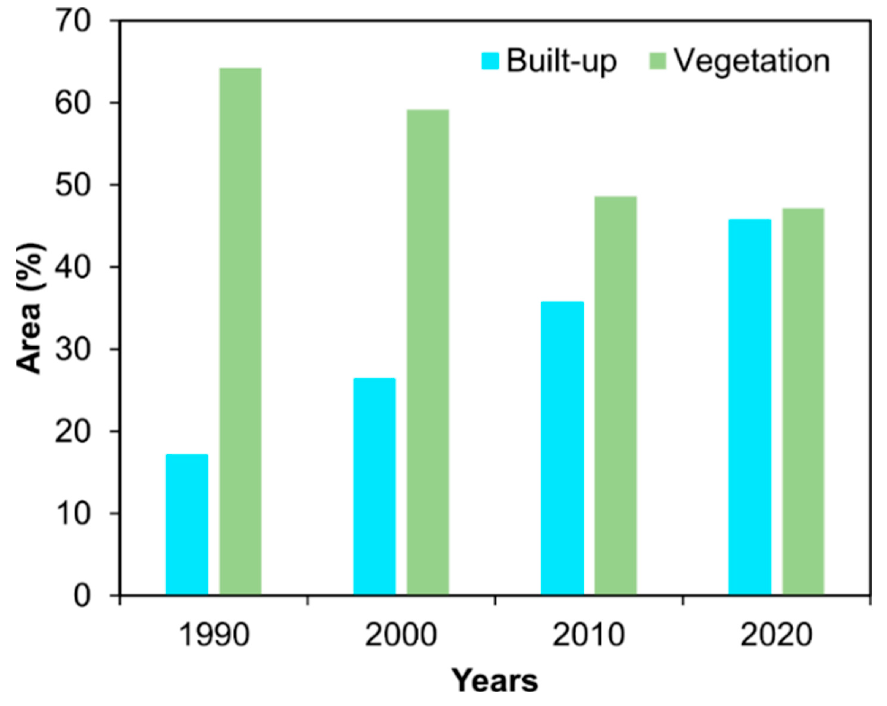
3.2. Land Cover Statistics and Change Rate

A significant reduction in the vegetated area and bare soil, and an increase in the built-up area, was observed between 1990 and 2020. A clear spatial variation, especially in vegetated areas and built-up areas, was observed due to the growth of the population throughout the study site, probably because of oil industry production.

Table 3. A summary of area coverage of LULC classes over the 30 year study period.

LU/LC Types	1990		2000		2010		2020
	Area (sq.km)	%	Area (sq.km)	%	Area (sq.km)	%	Area (sq.km)	%
Vegetation	117.08	64.24	107.76	59.13	88.52	48.57	85.91	47.14
Built-up	31.25	17.15	48.23	26.46	65.13	35.74	83.48	45.81
Bare land	10.44	5.73	15.98	8.77	14.88	8.17	4.88	2.68
Sand dunes	23.47	12.88	10.27	5.64	13.70	7.52	7.97	4.37

shows the resultant LULC change statistics, along with the change areas per sq.km and percentage. With reference to Table 1, it was observed that the vegetated area dropped by nearly 17.1% (i.e., 31.17 km²) over the 30 years, and similarly, bare land reduced by approximately 3.05% (i.e., 5.56 km²). This reduction was due to the rapid increase in urbanization at the study site, where the built-up area expanded from 17.15% in 1990 to 45.81% in 2020.

Figure 4 shows a comparison of annual vegetation cover change and built-up areas. Declining and increasing trends in vegetation and built-up areas can be observed over 30 years. It should be noted that since the early 1990s, the human influence began to play a significant role in environmental changes through reducing and fragmenting the area of green cover over Al-Ahsa Oasis.

3.3. Estimation of LST

With the aim of identifying the amount and nature of the UHIs’ spatial distribution within the area, LST for the different surface covers was extracted from the thermal ranges of the Landsat satellite images using the equations mentioned previously (Equations (1)–(7)). Additionally, by utilizing values (μ) and (δ) of LST, the heat island density over the area was calculated for the observed period of time, every 10 years starting from 1990 to 2020. Through the results of the study, we found that the surface temperatures varied between 26 °C and 52 °C throughout the study period, given in terms of least and ultimate LST, respectively. The statistics obtained from the analysis of heat islands are shown in

Table 4. The assessment of intensity of UHIs over the multiple surface covers of the study area.

Year	Total LST Pixels					Urban LST			Rural LST
	min	max	µ	δ	$\mathit{\mu }+0.5\mathit{\delta }$	min	max	µ	min	max	µ	UHI-Intensity (°C)
1990	31.6	52.4	40.8	4.1	42.8	42.8	52.4	47.6	31.6	42.8	37.2	10.4
2000	26.4	48.3	38.2	3.6	39.9	39.9	48.3	44.1	26.4	39.9	33.2	10.9
2010	31.7	47.8	39.4	3.5	41.2	41.2	47.8	44.5	31.7	41.2	36.4	8.1
2020	36.3	53.7	45.6	3.1	47.1	47.1	53.7	50.4	36.3	47.1	41.7	8.7

, where it should be noted that the intensity of heat islands (which represents the difference between heat islands for urban areas and heat islands for suburbs) ranged between 10.4 °C in the year 1990 to 8.7 °C for 2020.

Figure 5 displays the heat islands’ spatial distribution over the study area during the observation time (1990–2020). The heat islands were centered over urban areas during the study period, specifically in the western, eastern, and northern parts of the study area, where urban complexes (represented by some of the main cities and villages that surround the oasis) are situated. On the other hand, heat islands with low values were centralized around the middle of the study area, where there is a lot of vegetation cover due to palm plantations in the region. Starting from 2010, some aggregation of vegetation cover in the middle of the oasis began to develop, which was often due to palm plantations. However, these vegetation spots have been subjected to urban invasion (Figure 5c,d) during the last 10 years, leading to the emergence of separate heat islands permeating the vegetation cover.

3.4. Analysis of NDBI

In this study, the resultant NDBI values ranged between −0.39 and 0.35 (

Table 5. Descriptive statistical information for NDBI and LST over the period of 1990 to 2020.

Years	NDBI				LST
	Min.	Max.	Mean	SD	Min.	Max.	Mean	SD
1990	−0.39	0.21	−0.06	0.12	31.6	52.4	40.8	4.1
2000	−0.33	0.23	−0.03	0.11	26.4	48.3	38.2	3.6
2010	−0.22	0.17	−0.03	0.10	31.7	47.9	39.4	3.5
2020	−0.39	0.35	−0.05	0.11	36.3	53.7	45.6	3.1

). The negative values represent an absence of built-up areas (mostly vegetated areas), while the positive values reflect the presence of built-up locations within the study area across all years. As stated by Sobrino et al. [65], a lower value of NDBI reflects scattered built-up areas, while higher values indicate a concentration of built-up areas. A hot spots analysis was conducted in order to detect any spatial autocorrelation (clustering) between the hot and cold spots, in addition to any outlier or non-significant spots for the NDBI values throughout the study site. The maximum value of NDBI (0.35) was found in 2020, and the lowest value (0.17) was found in 2010.

Moreover, in terms of mean values, in 1990, the area had the lowest mean for NDBI, while in 2000 and 2010, the mean values were the highest. The highest values of NDBI were concentrated in the east and the west portions of the study area, while the central and northern portions had the lowest NDBI values due to vegetation cover (mostly palm trees) in these areas. The highest value of the maximum LST (53.7 °C) was found in 2020, and the lowest value (48.3 °C) was found in 2000.

Furthermore, in terms of mean values, in 2000, the area had the lowest mean LST, while in 1990 and 2020, the mean values were the highest (Table 5). The highest LST was at the eastern and western portions of the study site, whereas the central and northern parts had the lowest LST values, also as a result of date palm trees at these sites of the study area.

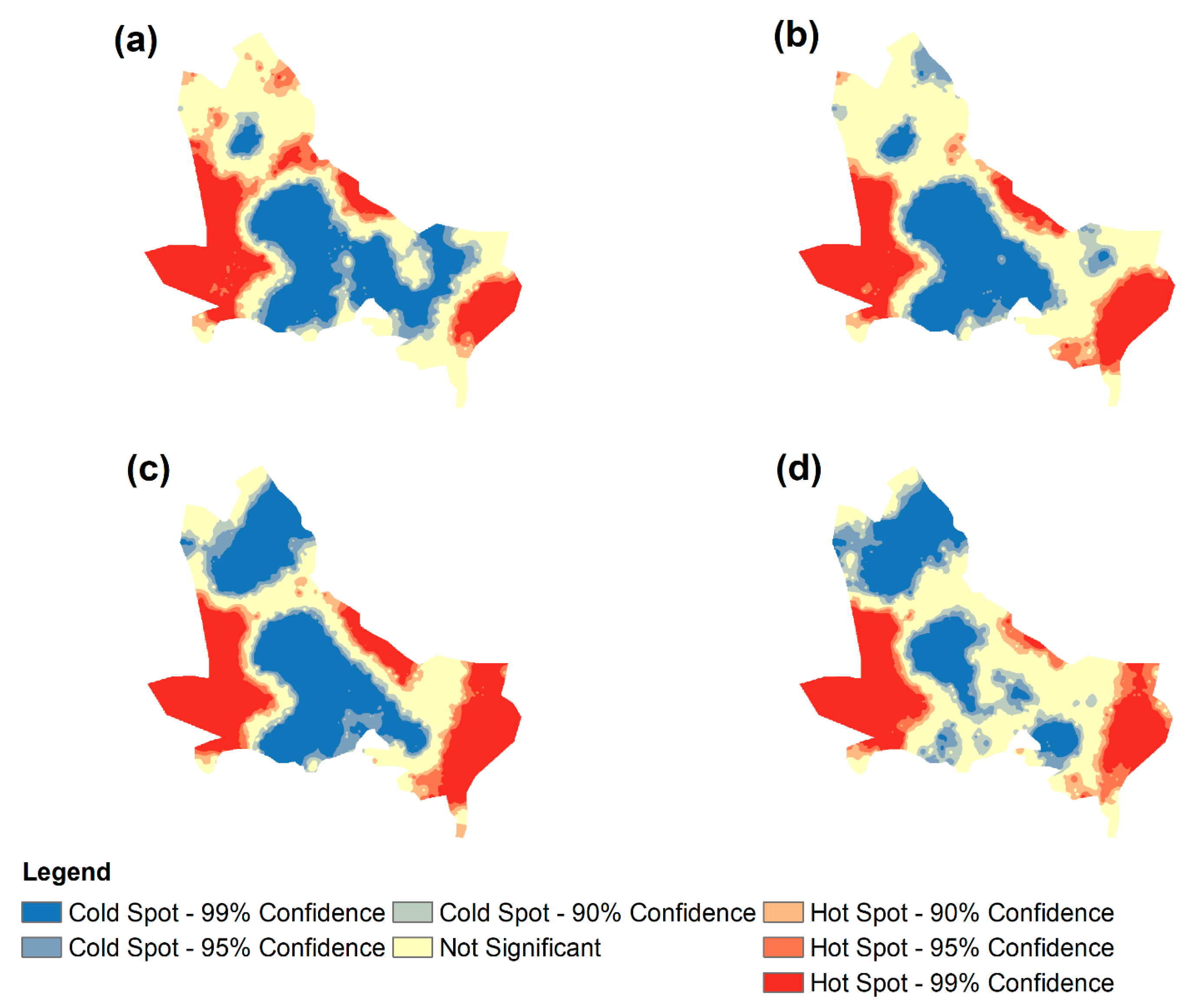
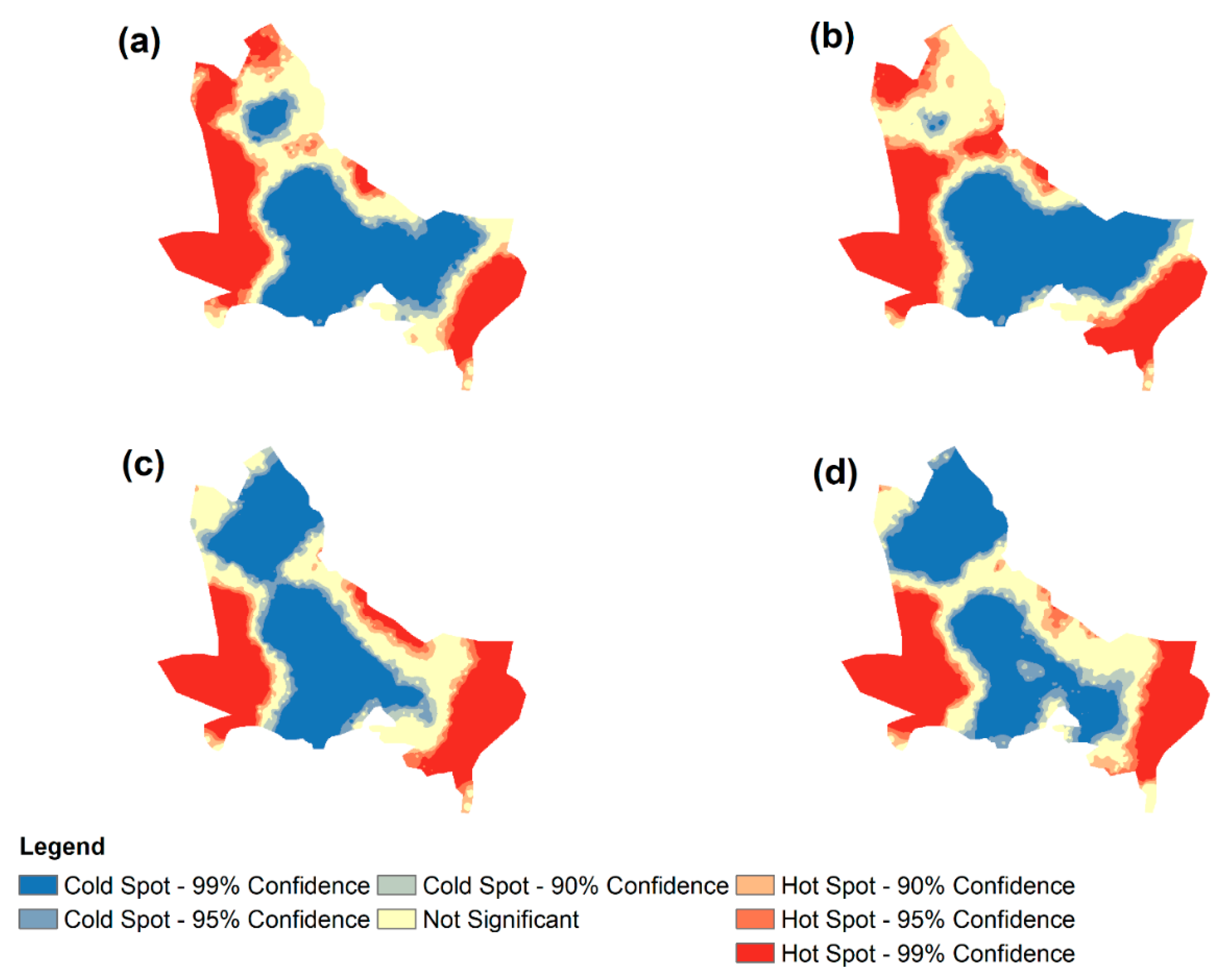
3.5. Analyzing the Spatial Pattern of NDBI and LST’s Hot and Cold Spots

Table 6. A summary of area coverage by hot, cold, and not-significant spots, along with Moran’s I values, for both NDBI and LST from 1990 to 2020.

Spot Type	NDBI				LST
	1990	2000	2010	2020	1990	2000	2010	2020
Cold Spot—99% Confidence	24.3	22.3	30.7	19	34.0	33.9	35.3	35.1
Cold Spot—95% Confidence	6.9	5.7	6.9	8.2	4.9	3.7	5.6	7.1
Cold Spot—90% Confidence	6.6	6.3	5.4	9.3	4.7	3.6	5.6	5.7
Not Significant	30.6	35.2	21.4	31.9	19.2	19.7	18.3	19.7
Hot Spot—90% Confidence	6.6	5.0	4.8	5.2	5.7	6.0	3.9	4.2
Hot Spot—95% Confidence	5.4	4.7	4.2	5.7	5.1	5.5	3.5	3.2
Hot Spot—99% Confidence	19.5	20.8	26.5	20.7	26.4	27.7	27.8	25.0
Moran’s I	0.409	0.385	0.486	0.322	0.639	0.605	0.604	0.615

The statistically significant level was set at p < 0.05.

lists the areas of NDBI and LST’s hot and cold spots, and their variations throughout the 30 years of the study time span. The spatial distribution of hot, cold, and non-significant spots for NDBI and LST is depicted in Figure 6a–d and Figure 7a–d. Generally, there was a moderate to high spatial autocorrelation (clustering) and statistical significance at p < 0.05 for both NDBI and the LST during the 30 years. The Moran’s I for the NDBI ranged from 0.322 to 0.486, while the LST ranged from 0.604 to 0.639 (Table 6).

High NDBI and LST values were categorized as hot spots, whereas small values were categorized as cold spot (Figure 6 and Figure 7). Hot spots of NDBI with 99% confidence ranged from 19.5% to 26.5% (Table 6). On the other hand, cold spots with 99% confidence ranged from 19% to 30.7%. The class of non-significant spots covered the largest area (35.2%) in 2000, versus the smallest (30.6%) in 1990. Regarding the analysis of LST’s hot spots, hot spots achieved their largest area (27.8%) in 2010 versus their lowest (25%) in 2020, though cold spots reached their maximum area (35.1%) in 2020 versus their lowest (33.9%) in 2000, with a 99% confidence level for all. Non-significant spot areas ranged from 18.3% to 19.7% over the study period.

When comparing the hot spot distribution of NDBI and LST, we found that most of the areas in the western, eastern, and the southeastern parts of the study area had experienced hot spots with 99% confidence. Areas within the center and towards the south, which were covered mostly with date palm plantations, had experienced zones of clustering of markedly cold spots, with a 99% confidence level. The areas characterized by spots that were not statistically significant were noticeably fragmented over the study area, with large portions in the northern parts for the years 1990 and 2000, and in the eastern parts for the years 2010 and 2020 (Figure 6 and Figure 7).

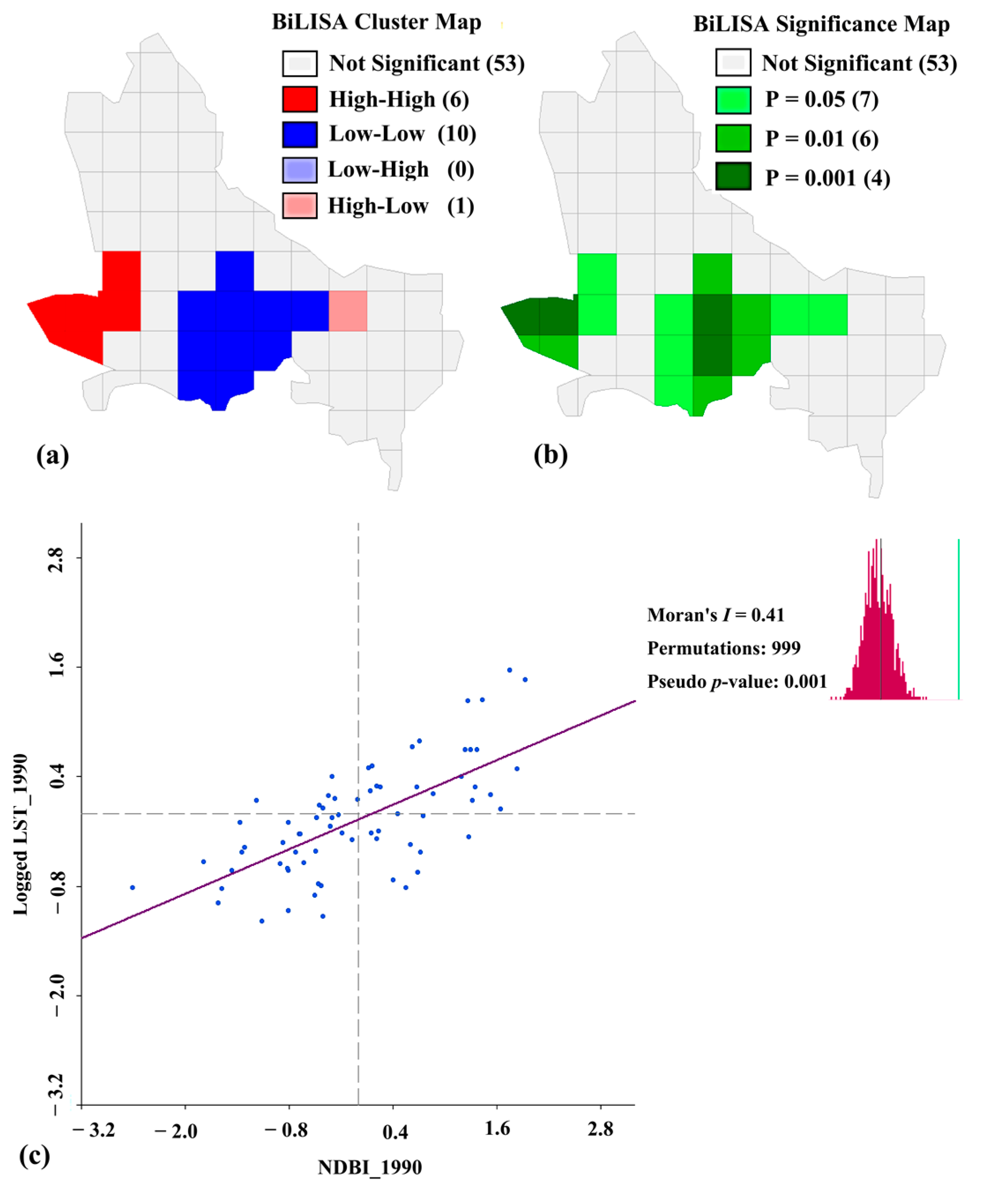
3.6. Depicting the Spatial Autocorrelation between Variation Patterns

As a way to reveal the possible agreement in the distribution forms between the spatially distributed LST and built-up areas (represented by NDBI), bivariate LISA and Moran’s I analysis approaches were employed. For Moran’s I, the vertical axis designated the neighboring grid values of LST, whereas the horizontal axis specified the average NDBI values. With respect to the study period (30 years), this analysis intended to examine the status of the spatial variability between the specified variables through considering pilot stages in terms of the year 1990, which was given as the starting period, and the year 2020, to represent the period’s end. For the year 1990, the resultant BiLISA clustering map, along with its specific significance for the spatially autocorrelated LST and NDBI and accompanied by Moran’s I, are presented in Figure 8a–c. Likewise, Figure 9a–c presents the spatial autocorrelation status represented by BiLISA clustering, as well as significance maps and Moran’s I for the year 2020.

The BiLISA spatial autocorrelation for the year 1990 revealed significant consistency between LST and NDBI (Figure 8a), wherein the proportion of high LST areas was mostly correlated with the high NDBI areas (high–high) and was dominant over the non-vegetated areas. In contrast, areas with low LST were observed to correlate with the lowest NDBI (low–low), and were centered over the oasis farm areas, with a significance (p-value) ranging between 0.05 to 0.001. However, some sporadic areas were occupied by a holistic surface cover type (farms, impervious surfaces, bare soils, etc.), resulting in insignificantly correlating grids (outliers) due to the mismatch between the vegetation, soil, and built-up surface covers within the 1 km² grid.

Furthermore, the 2020 applied BiLISA analysis (Figure 9a) also showed a significant positive (Figure 9b) correspondence (p-value between 0.05 and 0.001), indicated by high–high and low–low observed values over the urban and farm areas, respectively. Grids that had contributions of multi-surface cover formed a non-significant status. Moran’s I, which was utilized to assess the autocorrelation strength, had values of 0.41 and 0.45 for 1990 and 2020, respectively, with a permutations process of 999 plus 0.001 pseudo p-value for the two periods. It worth highlighting that the recently (2020) propagated (low–low) BiLISA zone, observed in the northern areas, was completely consistent with the change in the UHIs (Figure 5d) during the year 2020, particularly over the same geographical extent.

4. Discussion

Based on the nature of the spatial alignment between the urban areas and the heat islands, the temporal and spatial changes in LULC, especially built-up areas, can necessarily be summed up by a change in the spatial spreading of heat islands. The results of this study, in which the spatial autocorrelation technique was employed, was in agreement with many similar studies which had confirmed that urban expansion greatly contributes to increasing LST compared to green cover. For example, with reference to the impact of urban expansion over cities, Weng [66] determined that urban growth and reducing the vegetated area in the Zhujiang Delta in China from 1989–1997 elevated the surface temperature by an average of 13.01 °C. The temperature contrast between urban and rural areas increasing through urbanization has led to an increase in UHIs in some cities. Investigations into the increase of UHIs in the city of Tehran revealed that urbanization features directly affected the increase in daytime surface UHIs by 12 °C due to the difference between urban and non-urban maximum surface heat [58]. Hokao et al. [67] claimed that urban growth has increased the mean LST over Bangkok city from 26 ± 6 °C to 38 ± 3 °C in 2009. A much more substantial UHI influence of Shanghai resulted from urban growth, and it was identified as a primary cause of supplemental hot days and heat waves that increased heat-related deaths in the metropolis [68]. Zhang et al. [69] indicated that about 60% of the total LST variance was described by impervious surface areas (ISA) in relation to urban settlements within forest lands in mid-to-high latitudes worldwide. Li et al. [70] claimed a strong positive relationship between LST and ISA in Shanghai.

It is worth noting that urban growth at Al-Ahsa has incidentally influenced agriculture because of the rapid development. The most apparent reason for this was the oil exploitation in the region, which has brought about an escalation in urban area occupancy. Though the oil industry has led to direct occupation on the oilfields, unplanned service prospects have also emerged in towns all over the kingdom. Prior work has shown that the high rate of urban expansion has been a result of the fast growth in migration to the urbanized areas, as well as population growth [71], and its continuous increase towards agricultural land may transform the area into forests of cement and black surfaces [72]. On the other hand, the interplay of LULC and climatic variables (temperature, pressure, etc.) have had an impact on ecosystem evolution, as specified in earlier research [73] indicating that the temporal and spatial variations in LULC are the result of the underlying environmental impact of economic revolution. Abdelatti et al. [31] highlighted the danger of urbanization over Al-Ahsa green cover to the surrounding area. In addition, they argued that such urbanization, without considering the future, may lead to undesirable consequences for the local environment, as well as for community life.

Supporting the spatial autocorrelation between urbanization and LST over the study area, Buyadi [74] further suggested that variant kinds of LULC have variant LSTs, which is considerably affected by vegetation cover. Comparable results concerning LULC in the Al-Ahsa Oasis were likewise perceived by other researchers [31,75]. It is likely that demographic deviations triggered by urban development will ultimately lead to a destruction of land values [76]. This research concluded that changes in LULC caused by urbanization in the Al-Ahsa Oasis could have destructive effects on the area’s local climate.

The study findings also agreed with research outcomes achieved by Elsayed [36], who confirmed that temperature increases as the population grows. Further, the study demonstrated that there was an increase in temperature of 2.3 °C in the 10 year period between 2004 and 2014. It showed that there was a disparity in temperature intensity between different Al-Ahsa stations. Such a disparity in temperature confirms the existence of UHIs within the area. Other findings by Al-Ali [28] considering the arid nature of the Al-Ahsa Oasis have confirmed a very positive spatial correlation between LST, extracted from the thermal radiometers of Landsat 7 ETM+ and MODIS satellites, and the centralization of UHI intensity (10.55 °C) over the oasis’ major cities. It was observed that the UHI intensity was greater throughout the summer seasons compared to winter, and during night time as compared to day time.

5. Conclusions

This study was carried out with the aim of mapping, quantifying, and analyzing the spatiotemporal variation in UHIs over the arid Al-Ahsa area, in the Kingdom of Saudi Arabia. Additionally, it aimed to scope the extent of urban growth and its relative heat island effect from 1990 to 2020. The work was accomplished by quantifying the spatial variety of the UHIs, assessing the crucial factors and forms of the LST and NDBI distribution through space and time, and assessing the impact of LULC change on surface temperature throughout the 30 year period. The subsequent concluding points have been inferred as study findings:

• The technique of change detection was performed (with classification accuracies between 90 and 96%) to measure and map possible growth in urbanization and its effect on UHIs and UHI intensity quantification. The obtained change values revealed a considerable rate of growth in the urban area of 17.15% to 45.8% of the total LULC from 1990 to 2020, respectively.
• Considering the intensity of heat islands (which represents the difference between heat islands for urban areas and heat islands for suburbs), no abrupt variations were observed. The intensities ranged between 10.4 °C for 1990 and 8.7 °C for 2020.
• Taking into account the spatial distribution of UHIs, a remarkable consistency was observed throughout all study periods between NDBI and the LST, specifically over the western, eastern, and northern parts of the study site, where intense built-up complexes of main cities and villages are situated.
• A spatial autocorrelation analysis consisting of hot spots analysis and the BiLISA approach was implemented to identify particular relationships and clustering of variables. Further, it was intended to reveal the extent to which the nature of the association between the urban sprawl and UHIs can change. We found that most of the areas in the western, eastern, and southeastern parts (designated as built-up surfaces) had experienced hot spots, while areas covered with palm trees experienced clustering zones of cold spots, with 99% confidence for both. On the other hand, the BiLISA spatial autocorrelation revealed a significant consistency between LST and NDBI, with Moran’s I values of 0.41 and 0.45 for 1990 and 2020, respectively, with a significance (p-value) of 0.001 for all periods.

The spatiotemporal development in the built-up surfaces cover and its interaction with emissivity and LST could be employed as an assessment mechanism for the spatial fluctuation of metropolitan heat islands, which are considered a primary cause of supplemental hot days and heat waves that increase heat-related deaths in metropolis areas. However, this finding may be unique to the topographic, climatic, geographic, and environmental conditions in the Eastern region, where the study site was located. Co-occurring urbanization in other geographic regions may differ sufficiently to alter the UHI intensity and distribution. In addition, it is uncertain how UHI intensity and distribution may be affected by environmental conditions such as desertification. Future investigations will require a better understanding of factors controlling the long-term effects of urban development on UHIs. In particular, more comparisons of UHI intensity with sand encroachment or other types of land degradation are needed to determine how and under what circumstance these factors may differentially influence UHI patterns.

References

1. Rasul, A.O. Remote sensing of surface urban cool and heat island dynamics in Erbil, Iraq, between 1992 and 2013. Ph.D. Thesis, University of Leicester, Leicester, UK, 2016. [Google Scholar]
2. Oke, T.R. Boundary Layer Climates, 2nd ed.; Routledge: London, UK, 1987. [Google Scholar]
3. Lee, S.; French, S.P. Regional impervious surface estimation: An urban heat island application. J. Environ. Plan. Manag. 2009, 52, 477–496. [Google Scholar] [CrossRef]
4. Lee, J.S.; Kim, J.T.; Lee, M.G. Mitigation of urban heat island effect and greenroofs. Indoor Built Environ. 2014, 23, 62–69. [Google Scholar] [CrossRef]
5. Chow, W.T.; Brennan, D.; Brazel, A.J. Urban heat island research in Phoenix, Arizona: Theoretical contributions and policy applications. Bull. Am. Meteorol. Soc. 2012, 93, 517–530. [Google Scholar] [CrossRef] [Green Version]
6. Tarle, M. Application of GIS in Defining Urban Heat Island Using Transect Data: Urban Heat Island Using GIS Mapping; Lambert Academic Publishing: Saarbrücken, Germany, 2010. [Google Scholar]
7. U.S. Environmental Protection Agency. Urban Heat Island Basics. In Reducing Urban Heat Islands: Compendium of Strategies; U.S. Environmental Protection Agency: Washington, DC, USA, 2008. [Google Scholar]
8. Almulhim, A.I.; Bibri, S.E.; Sharifi, A.; Ahmad, S.; Almatar, K.M. Emerging Trends and Knowledge Structures of Urbanization and Environmental Sustainability: A Regional Perspective. Sustainability 2022, 14, 13195. [Google Scholar] [CrossRef]
9. Li, H.; Zhou, Y.; Li, X.; Meng, L.; Wang, X.; Wu, S.; Sodoudi, S. A new method to quantify surface urban heat island intensity. Sci. Total Environ. 2018, 624, 262–272. [Google Scholar] [CrossRef]
10. Kuang, W.; Liu, Y.; Dou, Y.; Chi, W.; Chen, G.; Gao, C.; Yang, T.; Liu, J.; Zhang, R. What are hot and what are not in an urban landscape: Quantifying and explaining the land surface temperature pattern in Beijing, China. Landsc. Ecol. 2015, 30, 357–373. [Google Scholar] [CrossRef]
11. Azevedo, J.A.; Chapman, L.; Muller, C.L. Quantifying the daytime and night-time urban heat island in Birmingham, UK: A comparison of satellite derived land surface temperature and high resolution air temperature observations. Remote Sens. 2016, 8, 153. [Google Scholar] [CrossRef] [Green Version]
12. Buyantuyev, A.; Wu, J.G. Urban heat islands and landscape heterogeneity: Linking spatiotemporal variations in surface temperatures to land-cover and socioeconomic patterns. Landsc. Ecol. 2010, 25, 17–33. [Google Scholar] [CrossRef]
13. Kamali Maskooni, E.; Hashemi, H.; Berndtsson, R.; Daneshkar Arasteh, P.; Kazemi, M. Impact of spatiotemporal land-use and land-cover changes on surface urban heat islands in a semiarid region using Landsat data. Int. J. Digit. Earth. 2021, 14, 250–270. [Google Scholar] [CrossRef]
14. Kumar, D.; Shekhar, S. Statistical Analysis of Land Surface Temperature–Vegetation Indexes Relationship Through Thermal Remote Sensing. Ecotoxicol. Environ. Saf. 2015, 121, 39–44. [Google Scholar] [CrossRef]
15. Yuan, F.; Bauer, M.E. Comparison of Impervious Surface Area and Normalized Difference Vegetation Index as Indicators of Surface Urban Heat Island Effects in Landsat Imagery. Remote Sens. Environ. 2007, 106, 375–386. [Google Scholar] [CrossRef]
16. Sultana, S.; Satyanarayana, A.N.V. Assessment of Urbanisation and Urban Heat Island Intensities Using Landsat Imageries During 2000–2018 Over a Sub-Tropical Indian City. Sustain. Cities Soc. 2020, 52, 101846. [Google Scholar] [CrossRef]
17. Grigoraș, G.; Urițescu, B. Land use/land cover changes dynamics and their effects on surface urban heat island in Bucharest, Romania. Int. J. Appl. Earth Obs. Geoinf. 2019, 80, 115–126. [Google Scholar] [CrossRef]
18. Atasoy, M. Assessing the impacts of land-use/land-cover change on the development of urban heat island effects. Environ. Dev. Sustain. 2020, 22, 7547–7557. [Google Scholar] [CrossRef]
19. Tran, H.; Uchihama, D.; Ochi, S.; Yasuoka, Y. Assessment with satellite data of the urban heat island effects in Asian mega cities. Int. J. Appl. Earth Obs. Geoinf. 2006, 8, 34–48. [Google Scholar] [CrossRef]
20. Hafner, J.; Kidder, S.Q. Urban Heat Island Modeling in Conjunction with Satellite-Derived Surface/Soil Parameters. J. Appl. Meteorol. 1999, 38, 448–465. [Google Scholar] [CrossRef]
21. Zhou, X.; Chen, H. Impact of urbanization-related land use land cover changes and urban morphology changes on the urban heat island phenomenon. Sci. Total Environ. 2018, 635, 1467–1476. [Google Scholar] [CrossRef]
22. Mochida, A.; Murakami, S.; Ojima, T.; Kim, S.; Ooka, R.; Sugiyama, H. CFD analysis of mesoscale climate in the Greater Tokyo area. J. Wind Eng. Ind. Aerodyn. 1997, 67, 459–477. [Google Scholar] [CrossRef]
23. Magee, N.; Curtis, J.; Wendler, G. The urban heat island effect at Fairbanks, Alaska. Theor. Appl. Clim. 1999, 64, 39–47. [Google Scholar] [CrossRef]
24. Li, D.; Liao, W.; Rigden, A.J.; Liu, X.; Wang, D.; Malyshev, S.; Shevliakova, E. Urban heat island: Aerodynamics or imperviousness? Sci. Adv. 2019, 5, 4299. [Google Scholar] [CrossRef] [PubMed] [Green Version]
25. Kumar, A.; Agarwal, V.; Pal, L.; Chandniha, S.K.; Mishra, V. Effect of Land Surface Temperature on Urban Heat Island in Varanasi City. India. J. 2021, 4, 420–429. [Google Scholar] [CrossRef]
26. Xian, G.; Shi, H.; Zhou, Q.; Auch, R.; Gallo, K.; Wu, Z.; Kolian, M. Monitoring and characterizing multi-decadal variations of urban thermal condition using time-series thermal remote sensing and dynamic land cover data. Remote Sens Environ. 2022, 269, 112803. [Google Scholar] [CrossRef]
27. Halder, B.; Bandyopadhyay, J.; Khedher, K.M.; Fai, C.M.; Tangang, F.; Yaseen, Z.M. Delineation of urban expansion influences urban heat islands and natural environment using remote sensing and GIS-based in industrial area. Environ. Sci. Pollut. Res. 2022, 29, 73147–73170. [Google Scholar] [CrossRef] [PubMed]
28. Al-Ali, A.M.H. The Effect of Land Cover on the Air and Surface Urban Heat Island of a Desert Oasis. Ph.D. Thesis, Durham University, Durham, UK, 2015. [Google Scholar]
29. Abdullah, H. The Use of Landsat 5 TM Imagery to Detect Urban Expansion and Its Impact on Land Surface Temperatures in the City of Erbil, Iraqi Kurdistan. Master’s Thesis, University of Leicester, Leicester, UK, 2012. [Google Scholar]
30. Al-Tahir, A.A.S. Al-Hassa: Geographic Study, 1st ed.; A-Hussainy Modern Press: Al-Hassa, Eastern Province, Saudi Arabia, 1999. [Google Scholar]
31. Abdelatti, H.; Elhadary, Y.; Babiker, A.A. Nature and Trend of Urban Growth in Saudi Arabia: The Case of Al-Ahsa Province–Eastern Region. Resour. Environ. 2017, 7, 69–80. [Google Scholar]
32. Elhadary, Y.A.; Al-Omair, A.A. Indicators and Causes of Rural Settlement Changes in Saudi Arabia: Alhasa Province in the Eastern District as Case Study. J. Gulf Arab. Penins. Studies. Gulf Arab. Penins. Stud. 2014, 155, 40. [Google Scholar]
33. Salih, A. Classification and mapping of land cover types and attributes in Al-Ahsaa Oasis, Eastern Region, Saudi Arabia Using Landsat-7 Data. J. Remote Sens. GIS. 2018, 7, 228. [Google Scholar] [CrossRef]
34. Alghannam, A.R.; Al-Qahtnai, M.R. Impact of Vegetation Cover on Urban and Rural Areas of Arid Climates. AJAE 2012, 3, 1–5. [Google Scholar]
35. Al-Zara, I.A. Elemental Composition of Groundwater and Spring Waters in Al-Ahsa Oasis, Eastern Region Saudi Arabia. Trends Appl. Sci. Res. 2011, 6, 1–18. [Google Scholar] [CrossRef] [Green Version]
36. Elsayed, I.S. A Study on Vulnerability of Alahsa Governorate to Generate Urban Heat Islands. Environ. Sci. Technol. 2016, 2, 392. [Google Scholar]
37. Congedo, L. Semi-automatic classification plugin documentation. Release 2016, 3, 29. [Google Scholar]
38. John, A.R. Remote Sensing Digital Image Analysis: An Introduction, 2nd ed.; Springer: New York, NY, USA, 1993. [Google Scholar]
39. Anderson, J. Land-use classification schemes used in selected recent geographic applications of remote sensing. Photogramm. Eng. Rem. Sens. 1971, 37, 379–387. [Google Scholar]
40. Pontius, R.G., Jr.; Millones, M. Death to Kappa: Birth of quantity disagreement and allocation disagreement for accuracy assessment. Int. J. Remote Sens. 2011, 32, 4407–4429. [Google Scholar] [CrossRef]
41. Stehman, S.V.; Foody, G.M. Key issues in rigorous accuracy assessment of land cover products. Remote Sens. Environ. 2019, 231, 111199. [Google Scholar] [CrossRef]
42. Olofsson, P.; Foody, G.M.; Herold, M.; Stehman, S.V.; Woodcock, C.E.; Wulder, M.A. Good practices for estimating area and assessing accuracy of land change. Remote Sens. Environ. 2014, 148, 42–57. [Google Scholar] [CrossRef]
43. Ashbindu, S. Review Article Digital change detection techniques using remotely-sensed data. Int. J. Remote Sens. 1989, 10, 989–1003. [Google Scholar]
44. Macleod, R.D.; Congalton, R.G. A quantitative Comparison of Change Detection Algorthms for Monitoring Eelgrass from Remotely Sensed Data. Photogramm. Eng. Remote Sens. 1998, 64, 207–216. [Google Scholar]
45. Fu, P.; Weng, Q. A time series analysis of urbanization induced land use and land cover change and its impact on land surface temperature with Landsat imagery. Remote Sens. Environ. 2016, 175, 205–214. [Google Scholar] [CrossRef]
46. Guo, G.; Zhou, X.; Wu, Z.; Xiao, R.; Chen, Y. Characterizing the impact of urban morphology heterogeneity on land surface temperature in Guangzhou, China. Environ. Model Softw. 2016, 84, 427–439. [Google Scholar] [CrossRef]
47. Landsat Project Science Office, Landsat 8 Science Data User’s Handbook. Available online: https://landsat.usgs.gov/documents/Landsat8DataUsersHandbook.pdf (accessed on 13 February 2022).
48. Sekertekin, A.İ.; Kutoglu, S.H.; Kaya, S. Evaluation of spatio-temporal variability in land surface temperature: A case study of Zonguldak, Turkey. Environ. Monit. Assess. 2016, 188, 30. [Google Scholar] [CrossRef]
49. Johansen, B.; Tømmervik, H. The relationship between phytomass, NDVI and vegetation communities on Svalbard. Int. J. Appl. Earth Obs. Geoinf. 2014, 27, 20–30. [Google Scholar] [CrossRef]
50. Silleos, N.G.; Alexandridis, T.K.; Gitas, I.Z.; Perakis, K. Vegetation indices: Advances made in biomass estimation and vegetation monitoring in the last 30 years. Geocarto. Int. 2006, 21, 21–28. [Google Scholar] [CrossRef]
51. Simwanda, M.; Manjula, R.; Ronald, C.E.; Yuji, M. Spatial Analysis of Surface Urban Heat Islands in Four Rapidly Growing African Cities. Remote Sens. 2019, 11, 1645. [Google Scholar] [CrossRef] [Green Version]
52. Pal, S.; Ziaul, S.K. Detection of Land Use and Land Cover Change and Land Surface Temperature in English Bazar Urban Centre. Egypt. J. Remote Sens. Space Sci. 2017, 20, 125–145. [Google Scholar] [CrossRef] [Green Version]
53. Traore, M.; Lee, M.S.; Rasul, A.; Balew, A. Assessment of land use/land cover changes and their impacts on land surface temperature in Bangui (the capital of Central African Republic). Environ. Chall. 2021, 4, 100–114. [Google Scholar] [CrossRef]
54. Zha, Y.; Gao, J.; Ni, S. Use of normalized difference built-up index in automatically mapping urban areas from TM imagery. Int. J. Remote Sens. 2003, 24, 583–594. [Google Scholar] [CrossRef]
55. Alonso, M.S.; Fidalgo, M.R.; Labajo, J.L. The urban heat island in Salamanca (Spain) and its relationship to meteorological parameters. Clim. Res. 2007, 34, 39–46. [Google Scholar] [CrossRef]
56. Shahmohamadi, P.; Ani, A.I.C.; Ramly, A.; Maulud, K.N.A.; Nor, M.F.I.M. Reducing urban heat island effects: A systematic review to achieve energy consumption balance. Int. J. Phys. Sci. 2010, 5, 626–636. [Google Scholar]
57. Effat, H.A.; Taha, L.G.E.; Mansour, K.F. Change detection of land cover and urban heat islands using multi-temporal landsat images, application in Tanta City, Egypt. Open J. Remote Sens. Position. 2014, 1, 1–15. [Google Scholar] [CrossRef]
58. Du, M.; Wang, Q.; Cai, G. Temporal and spatial variations of urban heat island effect in Beijing using ASTER and TM data. Urban Remote Sens. Event. 2009, 1–5. [Google Scholar]
59. Cheung, H.K.W. An Urban Heat Island Study for Building and Urban Design. Ph.D. Thesis, the University of Manchester, Manchester, UK, 2011. [Google Scholar]
60. Hove, L.W.A.V.; Steeneveld, G.J.; Jacobs, C.M.J.; Heusinkveld, B.G.; Elbers, J.A.; Moors, E.J.; Holtslag, A.A.M. Exploring the Urban Heat Island Intensity of Dutch Cities; Alterra report 2011, 2170 Alterra, part of Wageningen UR Wageningen; Alterra: Wageningen, The Netherlands, 2011. [Google Scholar]
61. Getis, A.; Ord, J.K. The analysis of spatial association by use of distance statistics. In Perspectives on Spatial Data Analysis; Springer: Heidelberg/Berlin, Germany, 2010; pp. 127–145. [Google Scholar]
62. Mitchel, A. The ESRI Guide to GIS analysis: Spatial measurements and statistics. In ESRI Guide to GIS Analysis; Esri: Redlands, CA, USA, 2005; Volume 2. [Google Scholar]
63. Exploring Spatial Data with GeoDa: A Workbook. Center for Spatially Integrated Social Science. Available online: http://csiss.org/clearinghouse/GeoDa/geodaworkbook.pdf (accessed on 15 March 2022).
64. Moran, P.A.P. Notes on Continuous Stochastic Phenomena. Biometrika 1950, 37, 17–23. [Google Scholar] [CrossRef]
65. Sobrino, J.A.; Jimenez-Munoz, J.C.; Paolini, L. Land surface temperature retrieval from LANDSAT TM 5. Remote Sens. Environ. 2004, 90, 434–440. [Google Scholar] [CrossRef]
66. Weng, Q. A remote sensing? GIS evaluation of urban expansion and its impact on surface temperature in the Zhujiang Delta, China. Int. J. Remote Sens. 2001, 22, 1999–2014. [Google Scholar]
67. Hokao, K.; Vivarad, P.; Manat, S. Assessing the impact of urbanization on urban thermal environment: A case study of Bangkok Metropolitan. Int. J. Appl. 2012, 2, 7. [Google Scholar]
68. Tan, J.; Zheng, Y.; Tang, X.; Guo, C.; Li, L.; Song, G.; Zhen, X.; Yuan, D.; Kalkstein, A.; Li, F.; et al. The urban heat island and its impact on heat waves and human health in Shanghai. Int. J. Biometeorol. 2010, 54, 75–84. [Google Scholar] [CrossRef]
69. Zhang, Y.; Odeh, I.O.; Han, C. Bi-temporal characterization of land surface temperature in relation to impervious surface area, NDVI and NDBI, using a sub-pixel image analysis. Int. J. Appl. Earth Obs. Geoinf. 2009, 11, 256–264. [Google Scholar] [CrossRef]
70. Li, J.; Conghe, S.; Lu, C.; Feige, Z.; Xianlei, M.; Jianguo, W. Impacts of landscape structure on surface urban heat islands: A case study of Shanghai, China. Remote Sens. Environ. 2011, 115, 3249–3263. [Google Scholar] [CrossRef]
71. Al-Jabr, M.A. Agriculture in Al-Hassa Oasis, Saudi Arabia: A Review of Development. Unpublished. Master’s Thesis, The Faculty of Social Sciences, University of Durham, Durham, UK, 1984. [Google Scholar]
72. Mohammed, H.A.; Elhadary, Y.A. Land Transport and Urban Expansion: Present Requirements and Future Challenges. A case Study on Al-Ahsa Province-Eastern Region-Saudi Arabia. J. Gulf Arab. Penins. Stud. 2020, 177, 46. [Google Scholar]
73. Barbier, E.B. Links between economic liberalization and rural resource degradation in the developing regions. Agric. Econ. 2000, 23, 299–310. [Google Scholar] [CrossRef]
74. Buyadi, S.N.A.; Wan, M.N.W.M.; Alamah, M. Impact of Land Use Changes on the Surface Temperature Distribution of Area Surrounding the National Botanic Garden, Shah Alam. In Proceedings of the International Conference on Quality of Life, Holiday Villa Beach Resort & Spa, Langkawi, Malaysia, 6–8 April 2013; pp. 516–525. [Google Scholar]
75. Al-Hussaini, Y.A. The use of multi-temporal Landsat TM imagery to detect land cover/use changes in Al-Hassa, Saudi Arabia. Sci. J. King Faisal Univ. (Basic Appl. Sci.) 2005, 6, 14–26. [Google Scholar]
76. Lambin, E.F.; Geist, H.J.; Lepers, E. Dynamics of land-use and land-cover change in tropical regions. Annu. Rev. Environ. Resour. 2003, 28, 205–241. [Google Scholar] [CrossRef] [Green Version]
Figure 1. Description of the workflow of the methodology used in this research.
Applsci 13 02755 g001
Figure 2. The geographical location of the study area.
Applsci 13 02755 g002
Figure 3. Classified images of LULC types: (a) 1990, (b) 2000, (c) 2010, and (d) 2020.
Applsci 13 02755 g003
Figure 4. The decadal change in vegetated area and built-up zones during the study period.
Applsci 13 02755 g004
Figure 5. The extracted UHIs over the study area for the periods (a) 1990, (b) 2000, (c) 2010, and (d) 2020.
Applsci 13 02755 g005
Figure 6. Change in hot and cold spots’ spatial patterns for NDBI during (a) 1990, (b) 2000, (c) 2010, and (d) 2020.
Applsci 13 02755 g006
Figure 7. Change in hot and cold spots’ spatial patterns for LST during (a) 1990, (b) 2000, (c) 2010, and (d) 2020.
Applsci 13 02755 g007
Figure 8. The resultant spatial autocorrelation between LST and NDBI, in which (a) represents BiLISA cluster, (b) significance maps, and (c) Moran’s I, for the year 1990.
Applsci 13 02755 g008
Figure 9. The resultant spatial autocorrelation between LST and NDBI, in which (a) represents BiLISA cluster, (b) significance maps, and (c) Moran’s I, for the year 2020.
Applsci 13 02755 g009