Researching and Predicting the Flow Distribution of Herschel-Bulkley Fluids in Compact Parallel Channels

Abstract

There is growing interest in multi-nozzle array printing, as it has the potential to increase productivity and produce more intricate products. However, a key challenge is ensuring consistent flow across each outlet. In the heat exchangers, achieving uniform distribution of flow in parallel channels is a classic goal. To address this issue in multi-nozzle array direct printing technology, high-viscosity slurry fluids can be utilized in place of water, and the structure of compact parallel channels can be employed. This study experimentally and numerically investigated the flow distribution law of Herschel-Bulkley fluids (high-viscosity slurry fluids) entering each manifold of the compact parallel channels, which contained a single circular inlet and multiple outlets. The research identified two types of factors that impact the non-uniformity flow coefficient (Φ), which reflects the uniformity of flow distribution in each channel of the structure: entrance and exit conditions (V, P₁, P₂) that have a negligible effect on Φ, and structural dimensions (D, S, L, N, A, d) that are the primary influence factors. By analyzing the experimental results, a prediction model was derived that could accurately calculate Φ (error < 0.05) based on three structural dimensions: A, S, and L. Through proper design of these structural dimensions, a consistent flow rate of each channel of the parallel channels can be ensured.

1. Introduction

Traditional printing technology with high-viscosity metal slurry fluids is gradually becoming unable to meet current work production needs due to cost, efficiency, and limitations of the process itself [1,2]. In order to achieve high-speed and cost-efficient printing, various new production and processing technologies have been explored, such as pattern transfer printing (PTP™) [3,4], flex trail-printing [5], laser chemical metal deposition [6], direct printing technology [7], and so on. In recent years, there has been growing interest in direct printing technology utilizing multi-nozzle arrays. The main challenge in this research is ensuring a uniform flow of high-viscosity metal slurry fluid across each channel, so as to ensure consistent flow at each channel or within an acceptable margin of error. The ultimate objective of this paper was to achieve uniform flow distribution in compact parallel channels.

Two main approaches exist in the structural study of multi-nozzle array direct printing with high-viscosity metal slurry fluids. The first approach, proposed by Chen [8,9], involved the use of a single syringe connecting 2 to 3 nozzles and controlling the extrusion of fluids through a valve. By juxtaposing multiple syringes, multi-nozzle array printing was achieved. To meet the need for more nozzles, Skylar-Scott et al. [10] designed a symmetrical structure to achieve multi-material, multi-nozzle 3D printing. However, due to the structure’s design, larger spacing between the nozzles was required that was not conducive to compact parallel printing, which limited its use. To solve the problem, the second approach involves the use of a box structure [11,12,13] with an inlet for feeding and pressure provided at the top of the box, while the required nozzle size and number are precision machined at the bottom for extrusion printing. Research indicated that homogeneous pressure and flow distribution within the print head was crucial in achieving homogeneous mass flow at all nozzles. However, the study had two drawbacks: (a) it did not explain how this structure affected the pressure distribution and ensured the smoothness and uniformity of the extrusion effect of each nozzle; (b) the integrated configuration of the structure may not be suitable for high-viscosity slurry fluids that are prone to clogging. Thus, there is a need to design a compact and detachable structure that can achieve uniform and smooth parallel printing, while explaining its flow behavior.

In the study of heat exchangers, in order to efficiently carry away the heat from a variety of extremely high temperature and high-pressure applications, researchers have designed U- and Z–type parallel multi-channel structures for uniform heat transfer. The current research contains the analysis of the causes and theory of non-uniform flow distribution in a manifold system [14,15,16], the influence of structural parameters on flow distribution [17,18,19,20,21], and the prediction of flow distribution in the heat exchangers [22,23]. Additionally, various inlet manifold structures are proposed to achieve uniform flow, including modified airfoil-type channels [24], a plate-fin shunt tube [25], and rectangular, trapezoidal, and triangular header structures [26]. In the study of the uniform flow of heat exchangers, the structure dimension is large and the fluids are mostly low-viscosity Newtonian fluids, such as water. The flow uniformity of non-Newtonian fluids in heat exchangers has rarely been investigated in the available literature.

Our study applied a multi-nozzle array of high-viscosity slurry fluids for direct printing technology by designing a compact parallel channel for consistent flow distribution in each channel. We studied the effects of inlet velocity (V), inlet pressure (P₁), outlet pressure (P₂), inlet diameter (D), channel diameter (d), area ratio (A), number of channels (N), channel spacing (S), and channel length (L) on the non-uniformity flow coefficient (Φ). Finally, we obtained a prediction model of A, S, and L to Φ in order to guide the structural design and help obtain the compact parallel channels needed to achieve the same or similar flow of high-viscosity slurry fluids in each nozzle of the compact parallel channels.

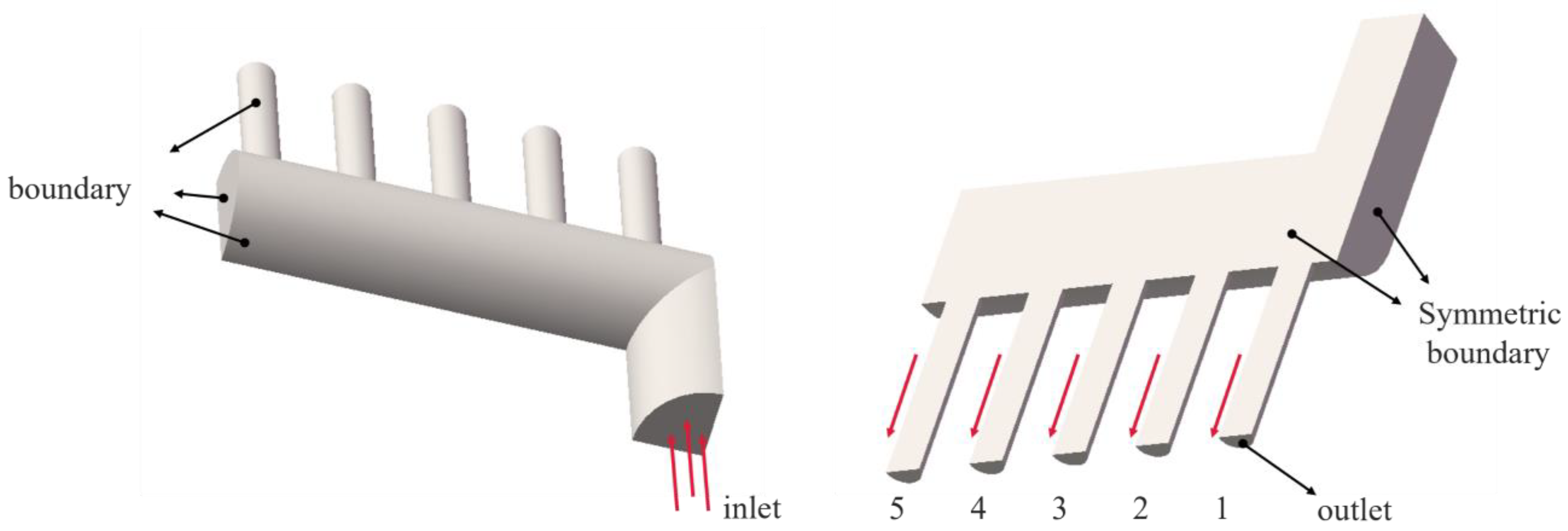
2. Physical Models

The structure of parallel channels designed according to the heat exchangers with a single circular inlet and multiple outlets is displayed in Figure 1. The entire fluids region consists of three parts: the inlet flow region, the fluid-filled cavity region, and the parallel channels fluids region. The following structural parameters are defined: inlet diameter (D), channel diameter (d), number of channels (N), channel spacing (S), and channel length (L).

The physical model shown in Figure 2 was used in the numerical simulation calculation where $N=10$. As a regular symmetric structure, the calculation process can be simplified and reduced by calculating only a quarter of the whole model. For the sake of description, the order from the center to the edge is 1 to 5. Subsequently, initial data was input into the numerical simulation, referring to Appendix B, including the geometry and dimensional parameters of the structure, inlet and outlet conditions (inlet velocity [V], inlet pressure [P₁], and outlet pressure [P₂]), fluid material parameters (density [$\rho$], viscosity [$\mu$], yield stress [${\tau }_0$], consistency [$K$], and Power-law index [$n$]).

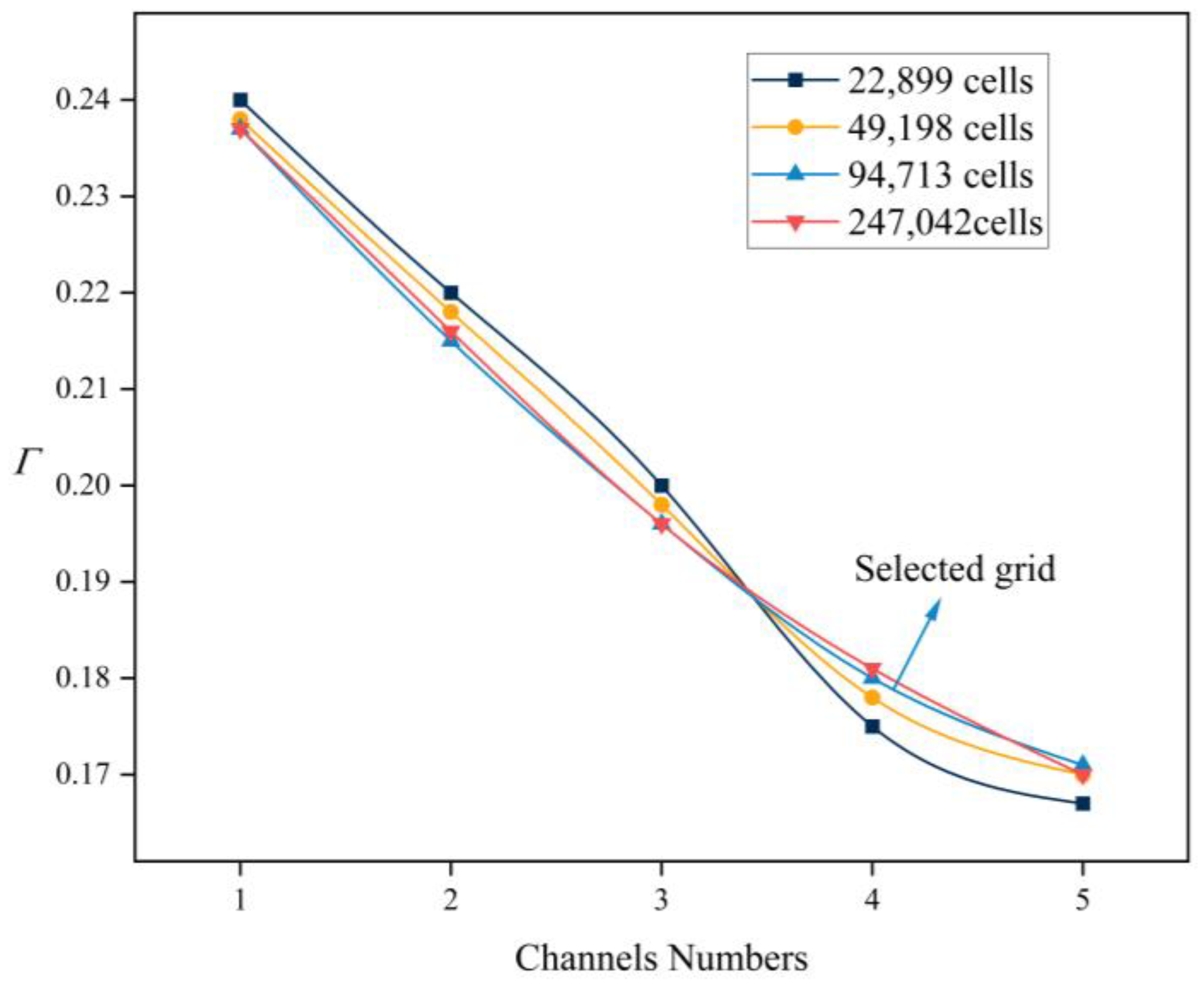
3. Numerical Simulation

After preliminary experimental research and theoretical analysis [18], the factors that affect fluid distribution in the compact parallel channels were mainly divided into two types. One set of factors was the inlet and outlet conditions: inlet velocity (V), inlet pressure (P₁), outlet pressure (P₂, which is atmospheric pressure with a value of 0.1 MPa), and pressure difference ($\Delta P=P_1-P_2$). Another set of factors was the structural dimensions: inlet diameter (D), channel diameter (d), area ratio (A), number of channels (N), channel spacing (S), and channel length (L). The following experiments were designed for the above parameters.

Defining the non-uniformity flow coefficient for analyzing flow distribution in the compact parallel channels, the uniformity of flow distribution in the structure can be intuitively reflected by:

$$\Phi =\frac{m_{\max }-m_{\min }}{\overline{m}}$$

(1)

The flow ratio is used for the analysis of flow distribution in each channel, which is defined as the ratio of flow rate in a single channel to the total flow rate, that is:

$$\Gamma =m/M$$

(2)

where $m$ is the mass flow rate in channel (kg/s), M is the total mass flow rate (kg/s), $m_{\max }$ is the maximum flow rate in channels, $m_{\min }$ is the minimum flow rate in channels, and $\overline{m}$ is the average flow rate of each channel. It can be seen that a smaller value of Φ represents more uniform flow of each channel. In this paper, because the structure was symmetrical, only N/2 channels were studied in the simulation, so the greater value of Γ tended to be 2/N, representing the more uniform flow of each channel.

This numerical simulation was conducted using the commercial software COMSOL Multiphysics® [27]. The peristaltic flow module (spf) under the single-phase flow module was applied in this study, the finite element method was employed to solve the CFD problem, and the CFD numerical model is shown in Appendix C. Grid independence was verified. As shown in Figure 3, the relative deviation of flow ratios between the grid with 94,713 cells and the densest grid with 247,042 cells was less than 1%, so the grid with 94,713 cells was adopted as the calculation grid.

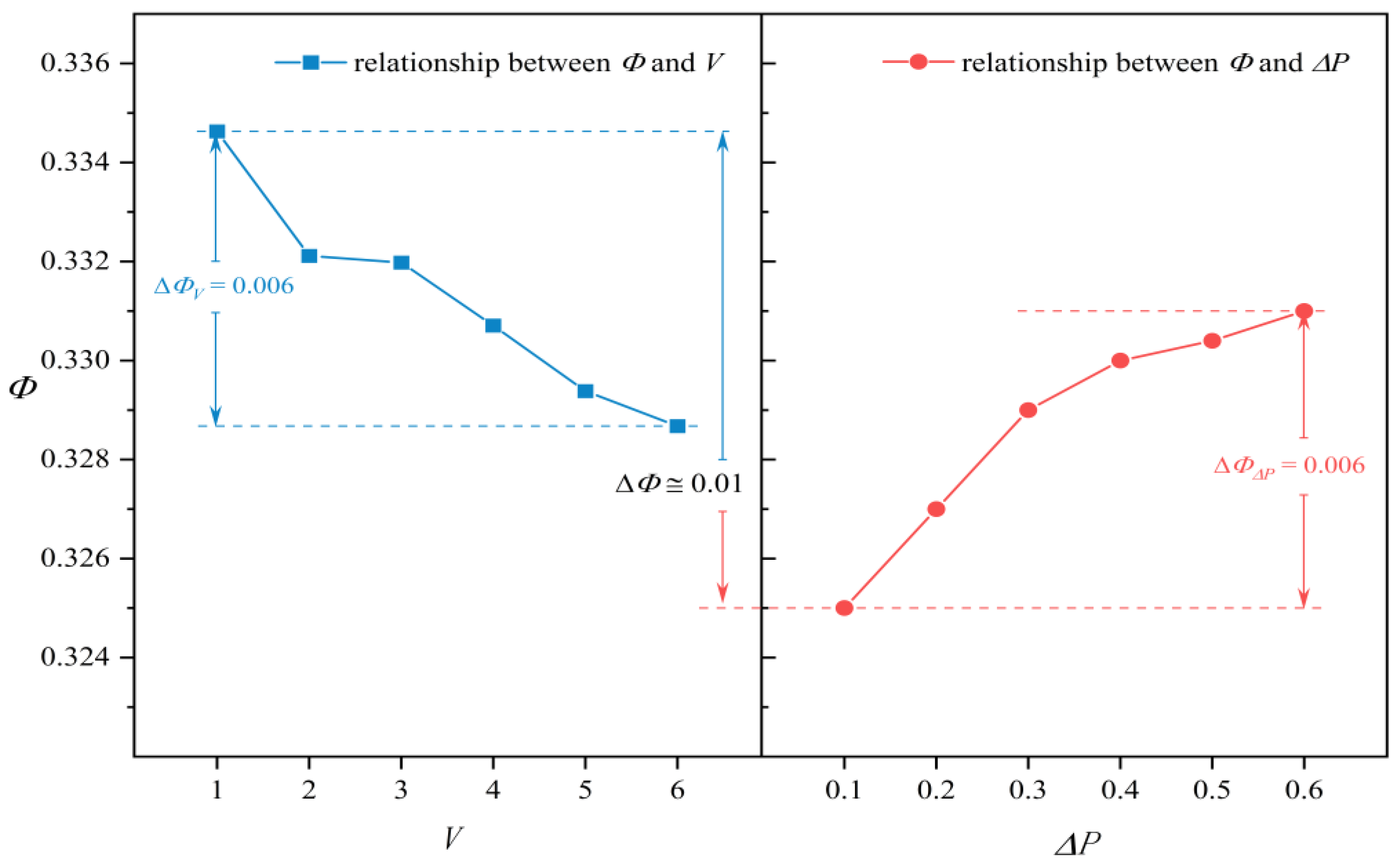
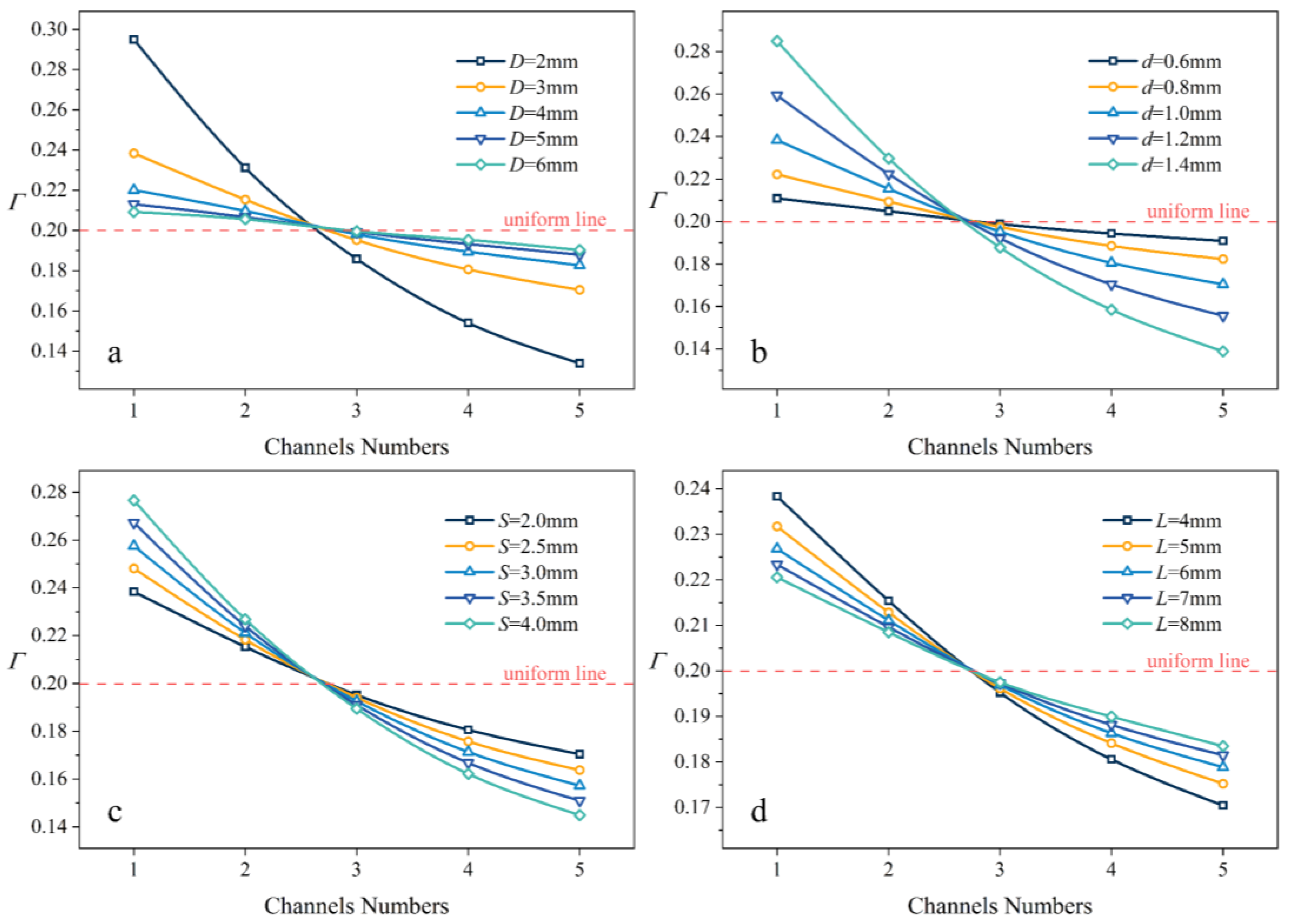
3.1. The Influence of Inlet and Outlet Conditions and Structural Parameters

Due to the research background being the flow distribution in a compact structure, the units of the structure parameters and inlet velocity were given in millimeters. The numerical simulation study of a single variable was carried out for the six parameters mentioned above, V, ∆P, D, d, S, and L, to analyze and determine the effect of changes in each parameter on Φ and Γ. The initial parameters were set as described in

Table 1. Parameter values.

Test Case	V [mm/s]	P2 [MPa]	D [mm]	d [mm]	S [mm]	L [mm]
1	[1:6:1]	0.1	3	1	2	4
2	0	∆P [0.1:0.6:0.1]	3	1	2	4
3	1	0.1	[2:6:1]	1	2	4
4	1	0.1	3	[0.6:1.4:0.2]	2	4
5	1	0.1	3	1	[2:4:0.5]	4
6	1	0.1	3	1	2	[4:8:1]

: $V=1$ mm/s, $\Delta P=0.1$ MPa, $D=3$ mm, $d=1$ mm, $S=2$ mm, and $L=4$ mm. The parametric values and conditions were based on experiments. At the beginning of the numerical simulation, the high-viscosity metal slurry fluids completely filled the entire structure. The dimensions of the structure were given in millimeters, and the velocity of flow was slow and measured in millimeters.

In the numerical simulation study of the parameters listed in Table 1, Figure 4 presents the results of test cases 1 and 2, while test cases 3–6 results are shown in Figure 5.

As can be seen from Figure 4, keeping other parameters constant and only changing the inlet velocity (V) resulted in the non-uniformity flow coefficient (Φ) slowly decreasing as V increased, indicating that the distribution of the flow in each channel tended to be uniform as V increased. Although Φ changed with V, the maximum difference was only $\Delta \Phi =0.006$. Similarly, the change in inlet and outlet differential pressure (∆P) had a similar phenomenon as the inlet velocity (V). The change in inlet velocity (V) and differential pressure (∆P) had negligible effects on the flow distribution in the compact parallel channels. This was consistent with the conclusion in ref. [16], that is, flow velocity was not the main factor affecting the flow distribution at low flow velocity conditions. Additionally, the difference between the two curves was extremely small, indicating that V and ∆P had similar influences on the results. Therefore, to reduce the calculation and combine with the actual conditions of this study, the subsequent numerical simulation used an inlet velocity $V=1$ mm/s and outlet pressure $P_2=0.1$ MPa.

The influences of the changes in inlet diameter (D), channel diameter (d), channel spacing (S), and channel length (L) on the flow ratio (Γ) are respectively given in Figure 5. Keeping other parameters constant and changing only D or L, the value of Γ for the same channel gradually decreased as the value of the parameters increased. This indicated that the flow distribution at each channel tended to be uniform, and the relationships between D and L and the variation of Γ showed a negative correlation. The results of transforming d and S were the opposite of the above; their relationships with the variation of Γ were positively correlated.

To sum up, in the structural design of the specified dimensional parameters within a certain range, in order to achieve uniform flow at each channel and reduce the value of the non-uniformity flow coefficient (Φ), the inlet diameter (D) and channel length (L) should be increased as much as possible, and the channel diameter (d) and channel spacing (S) should be reduced. In all cases, the flow at channel number 1 was the largest, and the flow at channel number 5 was the smallest. The results were different from those of Newtonian fluids, where the minimum pressure was at the channel near the inlet and the maximum pressure was at the end of the cavity region due to the jet effect at the inlet, resulting in minimum flow in the channels at the inlet and maximum flow in the end channels [18].

Pressure in the cavity region and parallel channels is the main factor leading to different flow distribution results. The fluid pressure in an entrance header will change for two reasons [28,29]: (a) because of wall friction in the straight sections between adjacent side outlets, the fluid pressure will fall in the flow direction; (b) the structural dimensions of parallel channels determine the pressure required for fluid to enter the channel, and fluid always tends to flow preferentially to areas with low flow resistance. When the flow resistance of the channel increases, the pressure at the entrance header of the channel increases, which will promote flow into the channel behind. This explains the effect of changes in structural parameters on the flow distribution.

To investigate the strength of the effect of the four structural parameters, D, d, S, and L, on Φ, we designed the orthogonal test as demonstrated in

Table 2. Orthogonal parameter table.

Factor/Level	D	d	S	L
	Inlet Diameter	Channel Diameter	Channel Spacing	Channel Length
1	3	0.8	2	2
2	4	1.0	3	4
3	5	1.2	4	6
4	6	1.4	5	8

, exploring the significance of the influence of the structural parameters. There were four factors to be investigated and each factor had four levels. The L16 (4⁴) orthogonal table was selected to schedule the numerical simulation.

Table 3. Analysis of variance for experimental results.

Factor	SS	df	MS	F
D	0.663	3	0.221	2.027
d	0.405	3	0.135	1.239
S	0.210	3	0.070	0.643
L	0.285	3	0.095	0.870
error	0.327	3	0.109

shows the parameters SS, df, MS, and F, which were obtained by calculating the numerical simulation result ${\mathit{x}}_i$ (in the study, $\mathit{x}=\Phi$). SS is the sum of squares of deviations, $\mathit{S}\mathit{S}={{\displaystyle \sum \left({\mathit{x}}_i-\overline{\mathit{x}}\right)}}^2$. df is the degree of freedom, df = k $-1$, where k is the number of factors. MS is the mean square, $\mathit{M}\mathit{S}=\frac{{\mathit{x}}_1^2+{\mathit{x}}_2^2+\cdots +{\mathit{x}}_{\mathit{n}}^2}{\mathit{n}}$. F is the F-test, $\mathit{F}\sim \mathit{F}\left(\mathit{k}-1,\mathit{n}-\mathit{k}\right)$, where n is the number of levels.

Sixteen groups of simulation experiments were designed and the results were analyzed for variance, as shown in Table 3. The results revealed that the strength of effect on the non-uniformity flow coefficient (Φ) in this experiment was: inlet diameter (D) > channel diameter (d) > channel length (L) ≈ channel spacing (S).

3.2. Prediction of the Influence of A, S, L on Φ Value

To the best of our knowledge, the non-uniformity flow coefficient (Φ) mainly depended on the inlet diameter (D) and channel diameter (d). The change in D and d refers to the change in the ratio of the sum of the channel cross-sectional area and the inlet cross-sectional area; therefore, the area ratio parameter (A) was defined to uniformly represent the variety of these two parameters and N, that is:

$$A=\frac{N·d^2}{D^2}$$

(3)

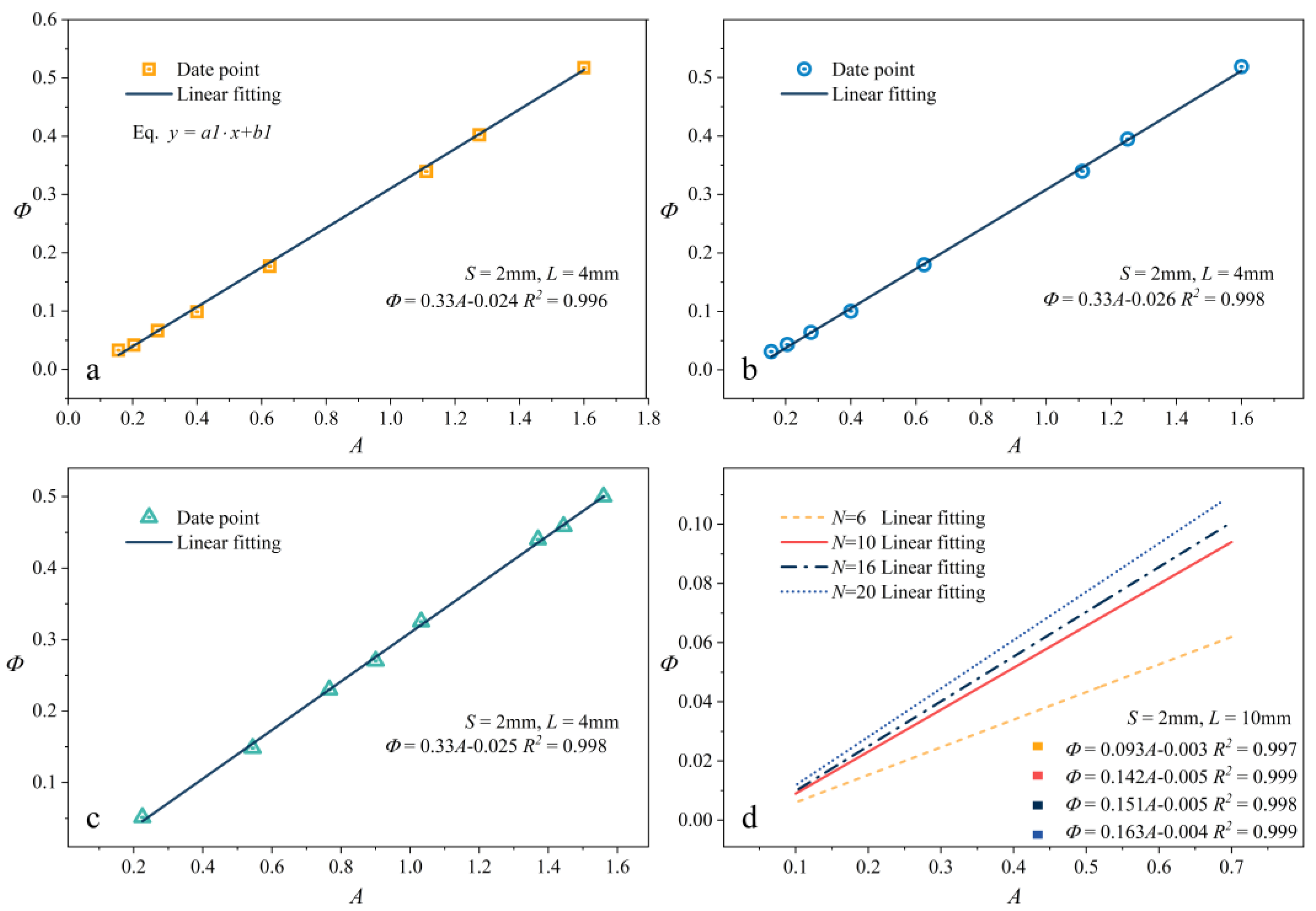
3.2.1. Study of the Functional Relationship between A and Φ

To study the functional relationship between A and Φ, with settings $S=2$ mm and $L=4$ mm, A contained three parameters: d, D, and N. Changing these three parameters separately gave the results displayed in Figure 6. It can be seen that as long as A was consistent, the relationship between A and Φ was linear and consistent. The relationship was given by:

$$\Phi =0.33A-0.025$$

(4)

When changing N and L, the relationship between A and Φ was also linear. As N increased, the slope increased, and the variation of S and L only affected the parameter term of the linear relationship. With increasing A and N, the non-uniformity of the flow distribution in each channel increased.

Therefore, when A was small, a relatively uniform flow distribution could be expected because a certain amount of momentum always required a corresponding friction to balance. For larger A, momentum could not balance the friction effect, resulting in non-uniform flow distribution. Thus, selecting the appropriate A could improve the uniformity of the pressure drop in the parallel channels. This was consistent with the conclusion in refs. [18,23].

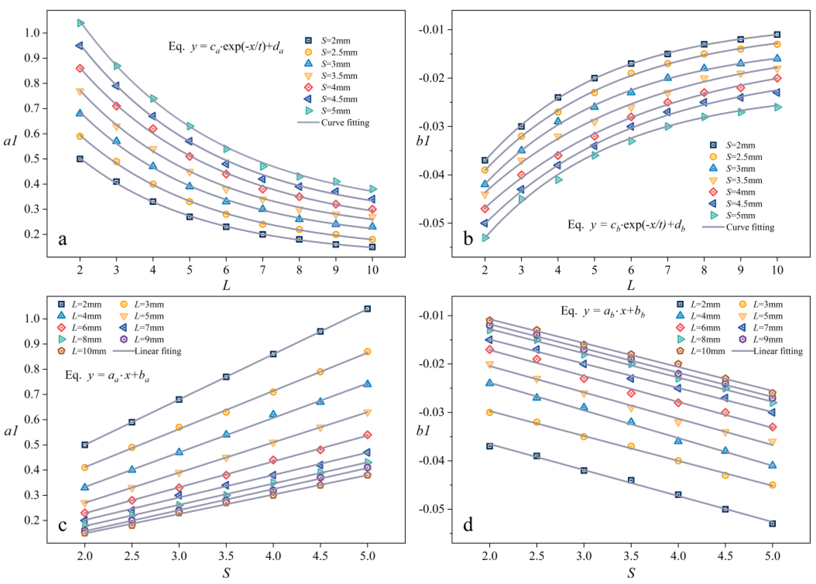
3.2.2. Study of the Functional Relationship between S, L, and Φ

Based on the research above, several conclusions may be drawn:

1. Φ and A have a certain linear relationship while S and L are determined.

2. When changing S and L, the primary term coefficient (a1) and constant term (b1) in the linear relationship vary in a regular manner.

Numerical simulation methods were used to study the numerical change in a1 and b1 with $2<S<5$ and $2<L<10$, as demonstrated in Figure 7. The linear relationship was given by:

$$\Phi =a1·A+b1$$

(5)

Figure 7a,b present the trends of a1 and b1, respectively, as L changed when S remained constant. It can be seen that the results of curve fitting was an exponential function, that is:

$$y=c·\exp \left(-x/t\right)+d$$

(6)

Figure 7c,d show the trends of a1 and b1, respectively, as S changed when L remained constant. The relationships were linear, given by:

$$a1=a_a·S+b_a$$

(7)

$$b1=a_b·S+b_b$$

(8)

The variations of a1 and b1 with S and L are displayed in Figure 8. The two functional relationships described above were unified, and a significant trend in numerical variation is shown. We know that smaller S and larger L will make smaller a1 and larger b1, thus causing uniform flow distribution in the parallel channels.

The linear relationship was analyzed and the results are summarized in Figure 9. The relationship between the primary term coefficient (a_a) and L was exponential (Figure 9a), given by:

$$a_a=0.2·\exp \left(-L/4\right)+0.06$$

(9)

The relationship between the primary term coefficient (a_b) and L was constant (Figure 9c) because the values all fluctuated around −0.0051. When −0.0051 was used instead, the maximum error after calculation of Φ was 0.00105. This is an acceptable value that has little effect on the calculation of Φ, so in this research we think:

$$a_b=-0.0051$$

(10)

The relationships between the constant terms b_a and b_b and L were exponential (Figure 9b,d), given by:

$$b_a=0.32·\exp \left(-L/3\right)-0.01$$

(11)

$$b_b=0.05·\exp \left(-L/3.2\right)+0.00123$$

(12)

Now, substituting each parameter into Equation (5), an approximate solution of Φ can be obtained:

$$\begin{array}{l}\Phi =\left\{\left[0.2·\exp \left(-L/4\right)+0.06\right]·S+0.32·\exp \left(-L/3\right)-0.01\right\}·A\\ -0.0051·S+0.05·\exp \left(-L/3.2\right)+0.00123\end{array}$$

(13)

In summary, the Herschel-Bulkley fluid flow distribution in the compact parallel channels had obvious regularity. In practical engineering applications, the complex fluids theory formula is abandoned and the flow distribution law of different fluids in different structures can be studied directly by numerical simulation calculation.

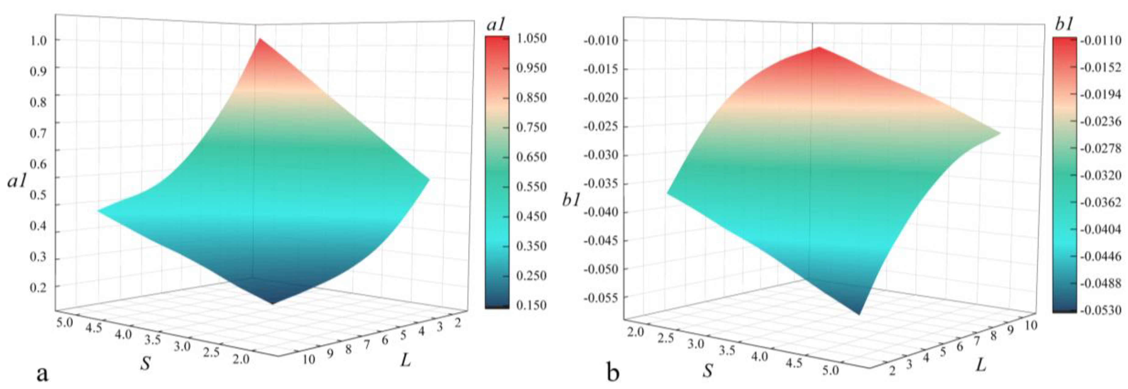
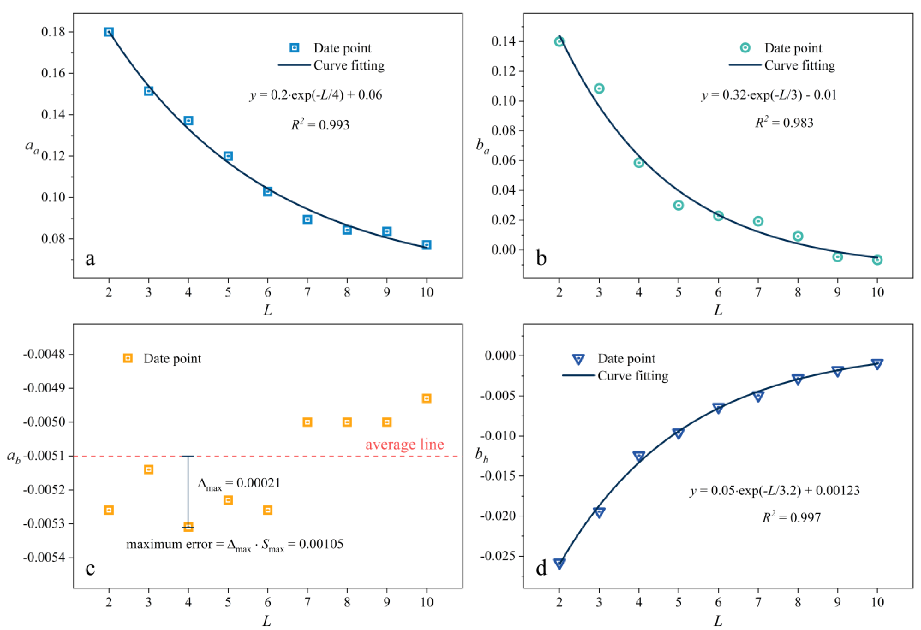
3.3. Prediction Model of Structural Parameters, A, S, and L, to Φ

It can be seen from the above that after knowing the structural dimensions D, d, S, and L of the compact parallel channels (referring to Figure 7 and Figure 9 or via calculation), we can know the primary term coefficient (a1) and constant term (b1) of the linear relationship between A and Φ. Then, A can be inserted into the linear relationship to obtain the predicted Φ. Predicting the flow distribution results in compact parallel channels with different structural parameters is of guiding significance.

In studying the accuracy of the prediction model in the range of $0<A<2.5$, $2<S<5$, and $2<L<10$, we designed 85 random groups of data with different structural parameters for simulation calculation and analyzed the results. Φ is the exact solution of the non-uniformity flow coefficient calculated by the simulation results, Φ_pr is an approximate solution of the non-uniformity flow coefficient calculated by the prediction model, and the error parameter (r) is defined to describe the error between the exact solution and the approximate solution, that is:

$$r=\left|\frac{\Phi -{\Phi }_{pr}}{\Phi }\right|$$

(14)

Figure 10 revealed the value of the error parameter (r) between the approximate solution (Φ_pr) and the exact solution (Φ), indicating that the error was mostly maintained within 0.1. Only when $0<\Phi <0.05$ would a very small number of points produce a large error ($r>0.1$). With increasing Φ, r gradually decreased, which indicated that the approximate solution was more accurate and A had no effect on the error. Because Φ is the non-uniformity flow coefficient of the compact parallel channels, when $0<\Phi <0.05$, even if the approximate solution error of a few points is $0.1<r<0.16$, the error of the prediction results was still within the acceptable range of the prediction model. Therefore, it can be considered that the exact solution (Φ) and approximate solution (Φ_pr) are basically the same with the same structural dimensions (A, S, L), showing that the prediction model was accurate for the prediction of the non-uniformity flow coefficient (Φ).

This study established a prediction model for flow distribution to simplify the calculation, as demonstrated in Figure 11. Through numerical simulation analysis, we could obtain the flow behaviors of fluids in the compact parallel channels, thereby guiding the design of the structure to meet the needs.

4. Experiment

The purpose of this experiment was to verify the flow distribution uniformity in each channel of the compact parallel channels, which was designed using the prediction model. The experimental method was to use the compact parallel channels for multi-nozzle array direct printing of the above high viscosity slurry fluids, attach needles of glass with nozzle diameters of 80 μm to the compact parallel channels, measure and calculate the cross-sectional area of the fluid line printed at each nozzle, and study the flow difference of each nozzle.

To control the flow difference of each nozzle within 5%, the compact parallel channels was designed using the prediction model: $N=10$, $D=5$ mm, $d=1$ mm, $S=2$ mm, and $L=10$ mm. The moving speed of the motion platform was $v=40$ mm/s, the inlet pressure was $P_1=0.4$ MPa, and the outlet pressure was $P_2=0.1$ MPa. The equipment of this experiment is shown in Figure 12. The computer controlled the movement and speed of the X and Y direction of the motion platform and controlled the Z direction movement of the bracket. The observation camera measured the distance between the glass nozzle and the motion platform, and the fluids were printed onto PET through glass nozzles under air pressure.

Figure 13 displayed the experimental results and analysis of the data. During the printing process, the existence of a drag-and-drop effect under the action of drag force and gravity resulted in the fluid lines having less width than the nozzle diameter. Dividing the experimental results into three groups for analysis, the flow of ten nozzles was nearly identical, $\Phi =0.046$. Due to the existence of the conical nozzle, the increased resistance in the channel was conducive to the uniform flow of each channel, and the Φ value measured and calculated in the experiment was less than the above predicted results. We believe that the compact parallel channels were successfully applied to multi-nozzle array printing.

Compared with the work of Chen et al. [8,9,10], this study implemented more parallel channels and greatly reduced the size of the device. More channels can also be extended in this study. In the study of Pospischil et al. [11,12,13], the influence of the device parameters on each outlet flow was unknown, which was solved in this paper.

5. Conclusions

This paper presents a fast and accurate prediction model to calculate the flow distribution in compact parallel channels in order to achieve uniform distribution of high-viscosity slurry fluid flow in compact parallel channels, which can be used in multi-nozzle array direct printing technology to make the flow in each nozzle consistent.

Through numerical simulation analysis and experiments, the study revealed the flow distribution law of Herschel-Bulkley fluids (high viscosity slurry fluids) in each manifold of the compact parallel channels, indicating the relationship between the non-uniformity flow coefficient Φ and parameters of the compact parallel channels. The main conclusions are as follows:

(1)

When the Herschel-Bulkley fluid flows slowly in the compact parallel channels, within the parameter range of this study, changes in V and ∆P have negligible effects on the fluid flow distribution in the compact parallel channels, and V and ∆P have similar effects on the results of flow distribution, thus we can choose one inlet velocity (V) and inlet pressure (P) to study.

(2)

The maximum flow occurs in channels near the inlet and at the minimum flow occurs at the end of the cavity region. The flow decreases sequentially and the results are different from those of Newtonian fluids. In order to create uniform flow at each channel, the inlet diameter (D) and channel length (L) should be increased and the channel diameter (d) and channel spacing (S) should be reduced as much as possible within the specified dimensional parameters of the structure design. The strength of the effect on the uniform flow is: inlet diameter (D) > channel diameter (d) > channel length (L) ≈ channel spacing (S).

(3)

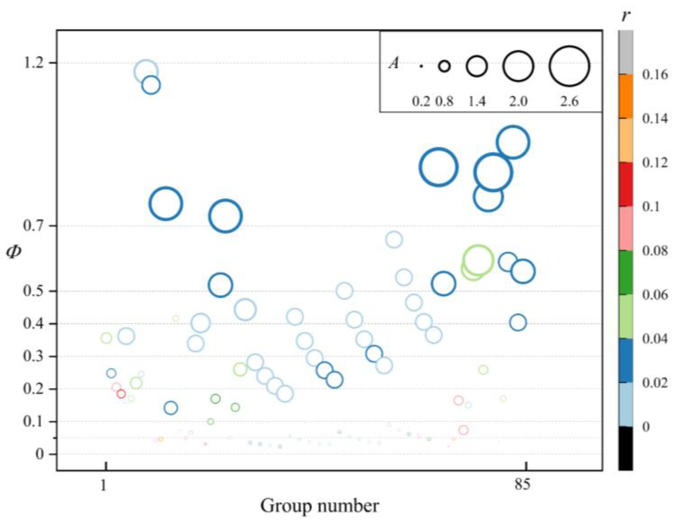
The non-uniformity flow coefficient (Φ) was defined to analyze the flow distribution in parallel channels, and the area ratio parameter (A) was defined to uniformly represent changes in the three parameters (N, D, d). According to Figure 10, Φ has a specific functional relationship with A, S, and L, which we can obtain by calculation. The functional relationship helps to design the compact parallel channel structure in order to achieve the specified flow difference.

The flow distribution theory of fluids in compact parallel channels is complicated and explaining all complex flows theoretically is difficult. The research methods and processes of this paper, which can be used to study the flow of other fluid models in compact parallel channels, can help improve the understanding of flow behaviors of fluids. Additionally, the prediction model provides easy-to-use design guidance in engineering applications. This study can also be used in multi-nozzle 3D printing, additive manufacturing, and so on. The flow distribution of more channels and more materials is a further research direction.

References

- Beaucarne, G.; Schubert, G.; Tous, L.; Hoornstra, J. Summary of the 8th workshop on metallization and interconnection for crystalline silicon solar cells. J. Green Sustain. Technol. 2019, 2156, 020001. [Google Scholar]
- Oreski, G.; Stein, J.; Eder, G.; Berger, K.; Bruckman, L.S.; Vedde, J.; Weiss, K.A.; Tanahashi, T.; French, R.H.; Ranta, S. Designing New Materials for Photovoltaics: Opportunities for Lowering Cost and Increasing Performance through Advanced Material Innovations. United States. 2021. Available online: https://www.osti.gov/biblio/1779380 (accessed on 10 January 2023).
- Lossen, J.; Matusovsky, M.; Noy, A.; Maier, C.; Bähr, M. Pattern Transfer Printing (PTP™) for c-Si Solar Cell Metallization. J. Energy Procedia 2015, 67, 156–162. [Google Scholar] [CrossRef]
- Mayberry, R.; Chandrasekar, V. Metallization contributions, requirements, and effects related to pattern transfer printing (PTP™) on crystalline silicon solar cells. Int. Symp. Green Sustain. Technol. ISGST 2019, 2156, 020008. [Google Scholar]
- Schube, J.; Fellmeth, T.; Jahn, M.; Keding, R.; Glunz, S.W. Advanced Metallization with Low Silver Consumption for Silicon Heterojunction Solar Cells. Int. Symp. Green Sustain. Technol. ISGST 2019, 2156, 020007. [Google Scholar]
- Wehkamp, N.; Fell, A.; Bartsch, J.; Granek, F. Laser chemical metal deposition for silicon solar cell metallization. J. Energy Procedia 2012, 21, 47–57. [Google Scholar] [CrossRef]
- Specht, J.; Zengerle, K.; Pospischil, M.; Erath, D.; Haunschild, J.; Clement, F.; Biro, D. High Aspect Ratio Front Contacts by Single Step Dispensing of Metal Pastes. In Proceedings of the 25th European Photovoltaic Solar Energy Conference and Exhibition, Valencia, Spain, 6–10 September 2010; pp. 1867–1870. [Google Scholar]
- Chen, X.; Church, K.; Yang, H. Highspeed non-contact printing for solar cell front side metallization. In Proceedings of the 2010 35th IEEE Photovoltaic Specialists Conference, Honolulu, HI, USA, 20–25 June 2010; pp. 1343–1347. [Google Scholar]
- Chen, X.; Church, K.; Yang, H.; Cooper, I.B.; Rohatgi, A. Improved front side metallization for silicon solar cells by direct printing. In Proceedings of the 2011 37th IEEE Photovoltaic Specialists Conference, Seattle, WA, USA, 19–24 June 2012; pp. 003667–003671. [Google Scholar]
- Skylar-Scott, M.A.; Jochen, M.; Visser, C.W.; Jennifer, A.L. Voxelated soft matter via multimaterial multinozzle 3D printing. J. Nat. 2019, 575, 330–335. [Google Scholar] [CrossRef] [PubMed]
- Pospischil, M.; Riebe, T.; Jimenez, A.; Kuchler, M.; Tepner, S.; Geipel, T.; Ourinson, D.; Fellmeth, T.; Breitenbücher, M.; Buck, T.; et al. Applications of Parallel Dispensing in PV Metallization. Int. Symp. Green Sustain. Technol. ISGST 2019, 2156, 020005. [Google Scholar]
- Pospischil, M.; Kuchler, M.; Klawitter, M.; Rodríguez, C.; Padilla, M.; Efinger, R.; Linse, M.; Padilla, A.; Gentischer, H.; König, M.; et al. Dispensing Technology on the Route to an Industrial Metallization Process. J. Energy Procedia 2015, 67, 138–146. [Google Scholar] [CrossRef]
- Pospischil, M.; Klawitter, M.; Kuchler, M.; Specht, J.; Gentischer, H.; Efinger, R.; Kroner, C.; Luegmair, M.; König, M.; Hörteis, M.; et al. Process Development for a High-throughput Fine Line Metallization Approach Based on Dispensing Technology. J. Energy Procedia 2013, 43, 111–116. [Google Scholar] [CrossRef]
- Zemlyanaya, N.V.; Gulyakin, A.V. Analysis of Causes of Non-Uniform Flow Distribution in Manifold Systems with Variable Flow Rate along Length. J. Mater. Sci. Eng. 2017, 262, 012098. [Google Scholar]
- Lee, S.; Moon, N.; Lee, J. A study on the exit flow characteristics by the orifice configuration of multi-perforated tubes. J. Mech. Sci. Technol. 2012, 26, 2751–2758. [Google Scholar] [CrossRef]
- Junye, W. Theory of flow distribution in manifolds. Chem. Eng. J. 2011, 168, 1331–1345. [Google Scholar]
- Ke, H.; Lin, Y.; Ke, Z.; Xiao, Q.; Xu, H. Analysis Exploring the Uniformity of Flow Distribution in Multi-Channels for the Application of Printed Circuit Heat Exchangers. Symmetry 2020, 12, 314. [Google Scholar] [CrossRef] [Green Version]
- Wang, C.-C.; Yang, K.-S.; Tsai, J.-S.; Chen, I.Y. Characteristics of flow distribution in compact parallel flow heat exchangers, part I: Typical inlet header. J. Appl. Therm. Eng. 2011, 31, 3226–3234. [Google Scholar] [CrossRef]
- Wang, C.-C.; Yang, K.-S.; Tsai, J.-S.; Chen, I.Y. Characteristics of flow distribution in compact parallel flow heat exchangers, part II: Modified inlet header. J. Appl. Therm. Eng. 2011, 31, 3235–3242. [Google Scholar] [CrossRef]
- Wei, M.; Fan, Y.; Luo, L.; Flamant, G. CFD-based Evolutionary Algorithm for the Realization of Target Fluid Flow Distribution among Parallel Channels. J. Chem. Eng. Res. Des. 2015, 100, 341–352. [Google Scholar] [CrossRef]
- Zhang, W.; Li, A.; Gao, R.; Li, C. Effects of geometric structures on flow uniformity and pressure drop in dividing manifold systems with parallel pipe arrays. Int. J. Heat Mass Transf. 2018, 127, 870–881. [Google Scholar] [CrossRef]
- Ma, T.; Zhang, P.; Shi, H.; Chen, Y.; Wang, Q. Prediction of flow maldistribution in printed circuit heat exchanger. Int. J. Heat Mass Transf. 2020, 152, 119560. [Google Scholar] [CrossRef]
- Camilleri, R.; Howey, D.; McCulloch, M. Predicting the flow distribution in compact parallel flow heat exchangers. J. Appl. Therm. Eng. 2015, 90, 551–558. [Google Scholar] [CrossRef]
- Cui, X.; Guo, J.; Huai, X.; Cheng, K.; Zhang, H.; Xiang, M. Numerical study on novel airfoil fins for printed circuit heat exchanger using supercritical CO2. Int. J. Heat Mass Transf. 2018, 121, 354–366. [Google Scholar] [CrossRef]
- Li, Y.; Li, Y.; Hu, Q.; Wang, W.; Xie, B.; Yu, X. Sloshing resistance and gas–liquid distribution performance in the entrance of LNG plate-fin heat exchangers. J. Appl. Therm. Eng. 2015, 82, 182–193. [Google Scholar] [CrossRef]
- Anbumeenakshi, C.; Thansekhar, M.R. Experimental investigation of header shape and inlet configuration on flow maldistribution in microchannel. J. Exp. Therm. Fluid Sci. 2016, 75, 156–161. [Google Scholar] [CrossRef]
- COMSOL Multiphysics® 5.6. cn.comsol.com. Guangxi University, Nanning, China.
- Pigford, R.L.; Ashraf, M.; Miron, Y.D. Flow distribution in piping manifolds. J. Ind. Eng. Chem. Fundam. 1983, 22, 463–471. [Google Scholar] [CrossRef]
- Choi, S.H.; Shin, S.; Cho, Y.I. The effect of area ratio on the flow distribution in liquid cooling module manifolds for electronic packaging. J. Int. Commun. Heat Mass Transf. 1993, 20, 221–234. [Google Scholar] [CrossRef]
- Balmforth, N.J.; Frigaard, I.A.; Ovarlez, G. Yielding to Stress: Recent Developments in Visco plastic Fluid Mechanics. J. Annu. Rev. Fluid Mech. 2014, 46, 121–146. [Google Scholar] [CrossRef]