Article

Strain Prediction Using Deep Learning during Solidification Crack Initiation and Growth in Laser Beam Welding of Thin Metal Sheets

1
Mathematics and Computer Science, Free University Berlin, 14195 Berlin, Germany
2
BAM—Bundesanstalt für Materialforschung Und-Prüfung, Fachbereich Schweißtechnische Fertigungsverfahren, 12205 Berlin, Germany
*
Authors to whom correspondence should be addressed.
Appl. Sci. 2023, 13(5), 2930; https://doi.org/10.3390/app13052930
Submission received: 1 February 2023 / Revised: 13 February 2023 / Accepted: 20 February 2023 / Published: 24 February 2023
(This article belongs to the Special Issue Advanced Diagnosis/Monitoring of Jointed Structures)

Abstract

:
The strain field can reflect the initiation time of solidification cracks during the welding process. The traditional strain measurement is to first obtain the displacement field through digital image correlation (DIC) or optical flow and then calculate the strain field. The main disadvantage is that the calculation takes a long time, limiting its suitability to real-time applications. Recently, convolutional neural networks (CNNs) have made impressive achievements in computer vision. To build a good prediction model, the network structure and dataset are two key factors. In this paper, we first create the training and test sets containing welding cracks using the controlled tensile weldability (CTW) test and obtain the real strain fields through the Lucas–Kanade algorithm. Then, two new networks using ResNet and DenseNet as encoders are developed for strain prediction, called StrainNetR and StrainNetD. The results show that the average endpoint error (AEE) of the two networks on our test set is about 0.04 , close to the real strain value. The computation time could be reduced to the millisecond level, which would greatly improve efficiency.

1. Introduction

Together with metallurgical factors, the formation of hot cracks during welding is mainly induced by the thermomechanical effect, which characterizes the strain-stress behavior of a material as a function of the temperature. The influence of the structure of the welded component and the stress intensity are also significant drivers of the hot cracking process. A variety of theories consider strain as an essential criterion for hot cracking. According to Pellini [1,2], hot crack initiation is based on strain localisation in the intercrystalline melt film. The tensile strains resulting from the welding process are transferred from the fully solidified region and the dendrites in the solidification region into the interdendritic melt films and accumulate there. Crack initiation occurs close to the solidus temperature as the grain boundaries are covered with thin melt films at this stage, and even small strains are sufficient for crack initiation. Prokohrov [3,4] defines the ’brittle temperature range (BTR)’. Within this temperature range, the weld metal reaches its minimum ductility during solidification. If the resulting strain exceeds the ductility of the crystallising melt, hot cracking occurs. Based on this basic idea, various authors have experimentally determined the maximum sustainable strain of this temperature range. Although the BTR concept only considers the mechanical component of hot cracking, it is particularly suitable for comparing different materials with regard to their susceptibility to hot cracking.
The experimental measurement of strain in the high-temperature range relevant for solidification cracking is usually difficult with the common measuring techniques, such as inductive displacement transducers or strain gauges. Besides the widely used strain gauge measurement method, modern optical technologies are increasingly used for non-contact measurements. Optical methods such as digital image correlation (DIC) do not require mechanical contact for taking measurements, so it is easy to obtain displacement data from the visible range of a digital camera. Unlike the use of strain gauges, these methods therefore have no influence on the processes being measured.
De Strycker et al. [5] were the first to use this technique to measure welding deformations. The strains estimated from the DIC technique were also compared with those obtained from the strain gauge (SG) technique, and the results showed good agreement. Using a digital camera and the normalized correlation algorithm, Shibabhara et al. [6,7] developed a two-dimensional (in-plane) technique to measure in-situ full-welding deformations. The further development of the measurement technique was reported in [8], where two digital cameras and the stereo imaging technique were used to match the images. Chen et al. [9,10] employed a similar setup to measure the strain during the gas tungsten arc welding (GTAW) process. Gollnow et al. [11] also utilized the DIC technique and the controlled tensile weldabilty test (CTW test) to analyze the weld pool near transverse displacements and the influence of this displacement on solidification crack formation. Gao et al. [12] used the free edge test to investigate the hot cracking susceptibility of TRIP steels; in that study, the DIC technique was also utilized to estimate the strain threshold required for hot crack formation. In their investigations, two 30 W LEDs with a wavelength of 450 nm were employed as an illumination source. A similar configuration was also used by Hagenlocher et al. [13] to determine the critical strain and strain rate threshold required for hot crack formation during the laser welding of aluminum alloys.
The optical flow technique has been used to estimate the motion of pixels in an image sequences [14]. Primarily, this technique is employed to estimate the object velocity and the position of the object in the next image. Moreover, it has found an important utilization in the field of experimental mechanics. [15,16]. The displacement field resulting from the application of optical flow has a subpixel resolution, usually with values less than 1 pixel. Gong and Bansmer [17] used the optical flow technique and image correlation to measure the deformation of a birdlike airfoil. The results show higher spatial resolution compared to the image correlation technique.
The DIC-based method can measure accurate displacement, but it is expensive and time-consuming. By integrating a digital camera into a laser head to film the moment of crack formation during laser beam welding for austenitic stainless steels and based on the optical flow technique, Bakir et al. [18,19] developed a 2-dimensional (2D) measurement technique that provides, for the first time, a local analysis of the strain field in the immediate vicinity of the solidification front.
Convolutional neural networks (CNN) [20] are one of the famous deep learning algorithms. They have achieved great success in per-pixel prediction problems due to their learning ability and high efficiency, supported by semantic segmentation, depth estimation, optical flow estimation, etc. Strain prediction can be regarded as a similar problem, especially when aiming at optical flow estimation, which learns correspondences between images. A milestone network FlowNet [21] first achieved the optical flow estimation based on deep learning. It adopts a generic U-Net architecture. The accuracy of FlowNet is still lower than traditional variational methods, so following FlowNet, many extensions have been developed to reduce the number of parameters and improve accuracy. In 2016, FlowNet2 [22] was proposed by stacking multiple subnetworks. The accuracy could be significantly improved at the cost of increased number of parameters and longer run time. SPyNet [23] incorporates the coarse-to-fine idea of the variational methods; it up-samples the learned flow and warps it on the second image to refine the flow. The model size is reduced, but the accuracy cannot compete with FlowNet2. The small and efficient network PWC-Net [24] is 17 times smaller than Flownet2 while maintaining high accuracy on several standard datasets; it leverages some simple but well-established principles from classical approaches, such as pyramidal processing, warping, and cost volume. Another concurrent work, LiteFlowNet [25], also adopts feature warping and proposes a novel flow regularization module. Subsequently, an increasing number of ideas emerged in optical flow estimation; IRR [26] adopts iterative optimization flow and weight sharing. H D 3 [27] introduces matching density estimation. VCN [28] improves the cost volume to 4D tensor. MaskFlownet [29] solves the occlusion problem. In 2020, a completely different network RAFT [30] was proposed. It removes the spatial pyramid structure and consists of three main components: a feature encoder, a correlation layer, and a recurrent update operator. This model has become a new milestone and is followed by many works [31,32,33,34].
Due to the success of deep learning in optical flow estimation, some CNN based methods can now retrieve displacement and strain fields as traditional DIC. They overcome its disadvantages, such as long computation time. Ref. [35] compares two image crack segmentation methods: the first applies a threshold on the strain map derived from the DIC, and the other uses a deep convolutional neural network. Boukhtache et al. [36] develops a network named StrainNet by modifying the number of down-samplings of FlowNet. It can obtain the full-resolution displacement and strain fields from reference and deformed speckle images. Yang et al. [37] proposed a deep learning method, Deep DIC, which includes two models, DisplacementNet and StrainNet, for displacement and strain prediction. The two models are slightly different in depth and up-sampling operation. The prediction results are highly consistent with commercial DIC software. In [38], a Hermite dataset is created to simulate deformation. Then, a new network DIC-Net on this dataset is trained that can successfully predict the strain field. [39] applies the image-segmentation technique DeepLabv3+ to achieve the pixel level classification of DIC strain field images, thus realizing damage detection in carbon-fiber-reinforced plastic (CFRP).
However, the above investigations have not been applied in laser beam welding. In this paper, we first collect a real welding dataset for training a good model. The controlled tensile weldability (CTW) test is a technique to crack the specimen through the external load; it is used to simulate the occurrence of cracks during the data generation. Then, the strain fields are calculated through a strain calculation method applying the OpenCV library [18,19]. The mechanisms of cracking during laser beam welding have been investigated in previous studies using the mentioned test and the strain measurement method based on an optical flow algorithm [18,40]. On the other hand, these existing models contain a large number of parameters, reaching up to tens of millions, which occupy a lot of memory. Moreover, there is the risk of overfitting our welding dataset. Two end-to-end models based on the U-Net [41] structure are developed. They adopt ResNet [42] and DenseNet [43] as the backbone for feature extraction and are named StrainNetR and StrainNetD. Finally, the performances of the two models are systematically analyzed; the results show that they achieve near-real-time strain prediction with a low error during the welding process, and the location of the identified cracks matches the real data.
The contributions of this paper are as follows:
  • A video of strained welding using CTW was generated;
  • Two deep neural networks called StrainNetR and StrainNetD for strain prediction were proposed;
  • The two models were trained and evaluated on the real generated dataset.

2. Methods

In this section, the methodology to generate a realistic welding dataset and the corresponding strain fields is introduced first. Then, the design of two strain prediction models is described.

2.1. Data Collection

The overall method of dataset generation includes three steps: conducting welding experiments, collecting images from the camera, and calculating the strain fields. The details are described as follows.

2.1.1. Welding under External Strain

The welding experiments were carried out with the Trudisk 16,002 disk laser from Trumpf, with a maximum output power of 16 kW, a wavelength of 1030 nm, and a beam parameter product of 8 mm x mrad. The welding experiments were carried out on sheets of austenitic steel grade 1.4404 (AISI 316 L) with a thickness of 2 mm. The chemical composition of the material, determined using the spectral analysis, is summarized in the Table 1. The welding parameters applied were 2 kW laser power and a constant welding speed of 1.2 m/min, at a focus position of +5 mm. Argon with a flow rate of 20 l/min was used as shielding gas. In these experiments, all welds were bead-on-plate welds and the seam length was 100 mm.
The solidification cracks were generated during laser beam welding using the hot cracking test under external loading. This type of hot cracking test or so-called externally loaded hot cracking test was developed to induce cracking in the specimen by external load. The controlled tensile weldability test was used in these experiments, where the weld specimen was subjected to a predefined strain and strain rate perpendicular to the welding direction while welding (see Figure 1). The strain was not controlled during the welding process; only a predefined transverse displacement corresponding to the targeted strain was applied.
The welded specimens were subjected during welding to a strain of 7% at three different strain rates 4 s 1 , 6 s 1 and 8 s 1 . The strain was applied after 30 mm after the start of welding with the corresponding (strain rates). Afterwards, the applied strain was kept until the end of welding. Figure 2 shows, schematically, the CTW test procedure during the welding process.

2.1.2. Data Acquisition

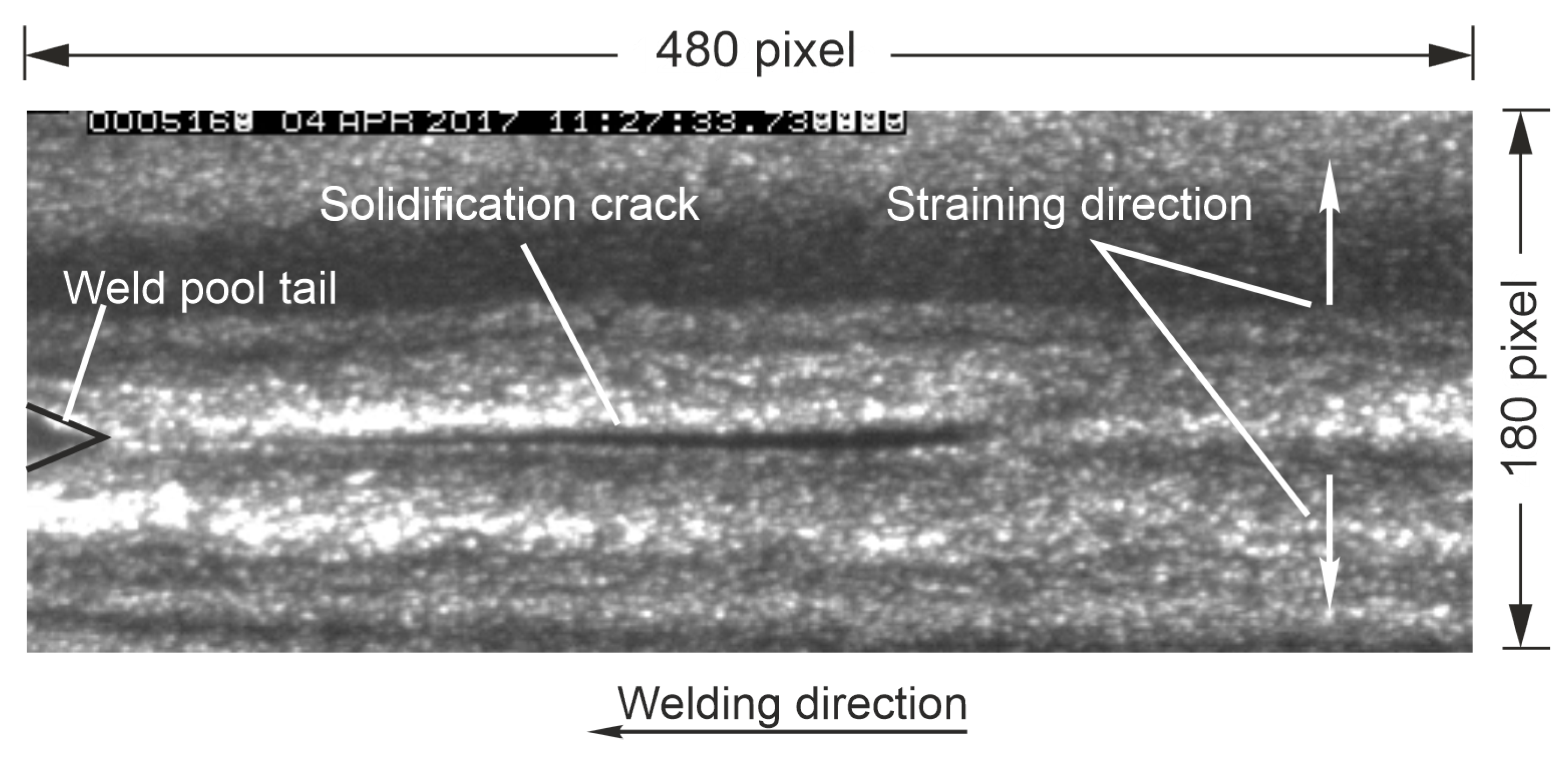
The video recording of the laser beam welding was performed with the PCO edge 5.5 camera, which has a sCMOS sensor Figure 1. The images were captured using a combination of external laser illumination and appropriate filters. A diode laser (compact diode laser) from Dilas with a wavelength of 808 nm and a maximum power of 100 W was used as the illumination source. The laser beam was guided by a fiber from the laser device to a collimator and finally projected by a beam expander on the sample surface. The selected interference filters have a mean wavelength of 808 nm and a bandwidth of 20 nm, ensuring that the optical filters will only pass the illumination wavelength and process emissions that have a wavelength of 808 nm. The process emissions that are not in the range of the illumination wavelength are suppressed. This enables a reliable recording with speckle pattern, which is helpful for strain estimation (see Figure 3). The recording rate used was 1176 fps. The images were stored in tif format with a resolution of 480 × 180 pixels.
Table 2 summarizes the prepared and used dataset and the data volumes. There are six videos, and each video contains around 5000 image sequences; four videos are called TD (training data), and two are called T (test). The training data amounts to 20,000 images. They are divided into a training set ( 80 % ) and a validation set ( 20 % ). The validation set is used to adjust the network structure and parameters. The test set consists of two different image sequences to evaluate the performance of the models.

2.1.3. Strain Estimation

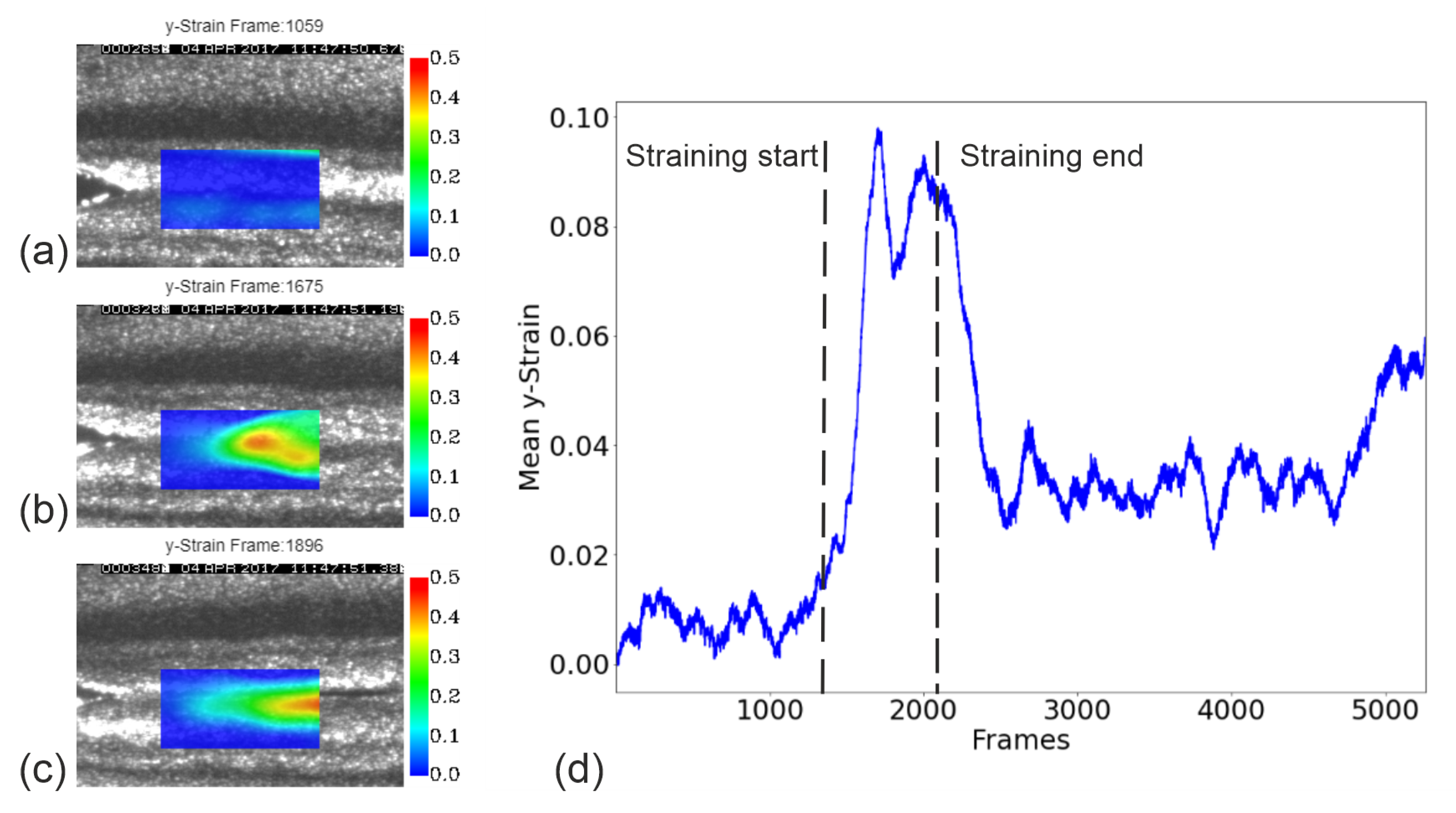
The strain estimation for solidified material is based on the work of Bakir et al. [18,19]. It uses the Lucas–Kanade algorithm [44] for optical flow. The pixels of the new solidified material (behind the melt pool) is included in the calculation, and it will be considered as long as the pixels are within the ROI (region of interest). After estimating the displacement between two frames, the calculated displacements are accumulated into a cumulative displacement field. Then, the Green–Lagrangian strain for each frame is calculated based on these accumulated displacements. The strain calculation software was developed using Python, in combination with OpenCV libraries. Figure 4 shows the perpendicular strain distribution to the welding direction in a selected region of interest behind the melt pool. The figure also shows the mean strain curve for the same region over the frame sequences.
The strain curve initially shows that the strain varies between 0 and 0.02 due to thermal expansion near the weld pool before an external load is applied. However, when an external load is applied (frame 1400), the strain response changes. Due to the accumulated external strain and thermal expansion working in the same direction, the strain increases rapidly. At frame 1675, the strain reaches its highest value, and this corresponds to the moment when the crack is initiated. Once the crack has formed, it propagates through the material and follows the solidification front. Due to crack propagation, the strain required is less than the strain for crack formation, so the strain correspondent decreases slightly. When the external load is stopped, the strain starts to decrease locally. Shortly thereafter, the strain falls below the critical threshold and fluctuates between 0.02 and 0.04. This behavior of the strain was discussed further in [19]. While ref. [19] considered different ROIs, the qualitative behavior of the strain is similar.

2.2. Neural Network Model Architecture

The calculation based on optical flow can obtain accurate results, but it takes a long time to process each image pair. In this section, the use of neural networks to provide results faster and reduce the computational cost is investigated. The strain-prediction model adopts the encoder-decoder structure as shown in Figure 5. The encoder consists of several successive convolutional layers to extract features from image pairs. The decoder is symmetric to the encoder, and it can recover the strain field from narrow feature maps. The network FlowNet [21] has been explored before. In this paper, its encoder is optimized with two classic networks: ResNet and DenseNet, respectively. The decoder is also modified to obtain the full-resolution strain field.

2.2.1. The Encoder

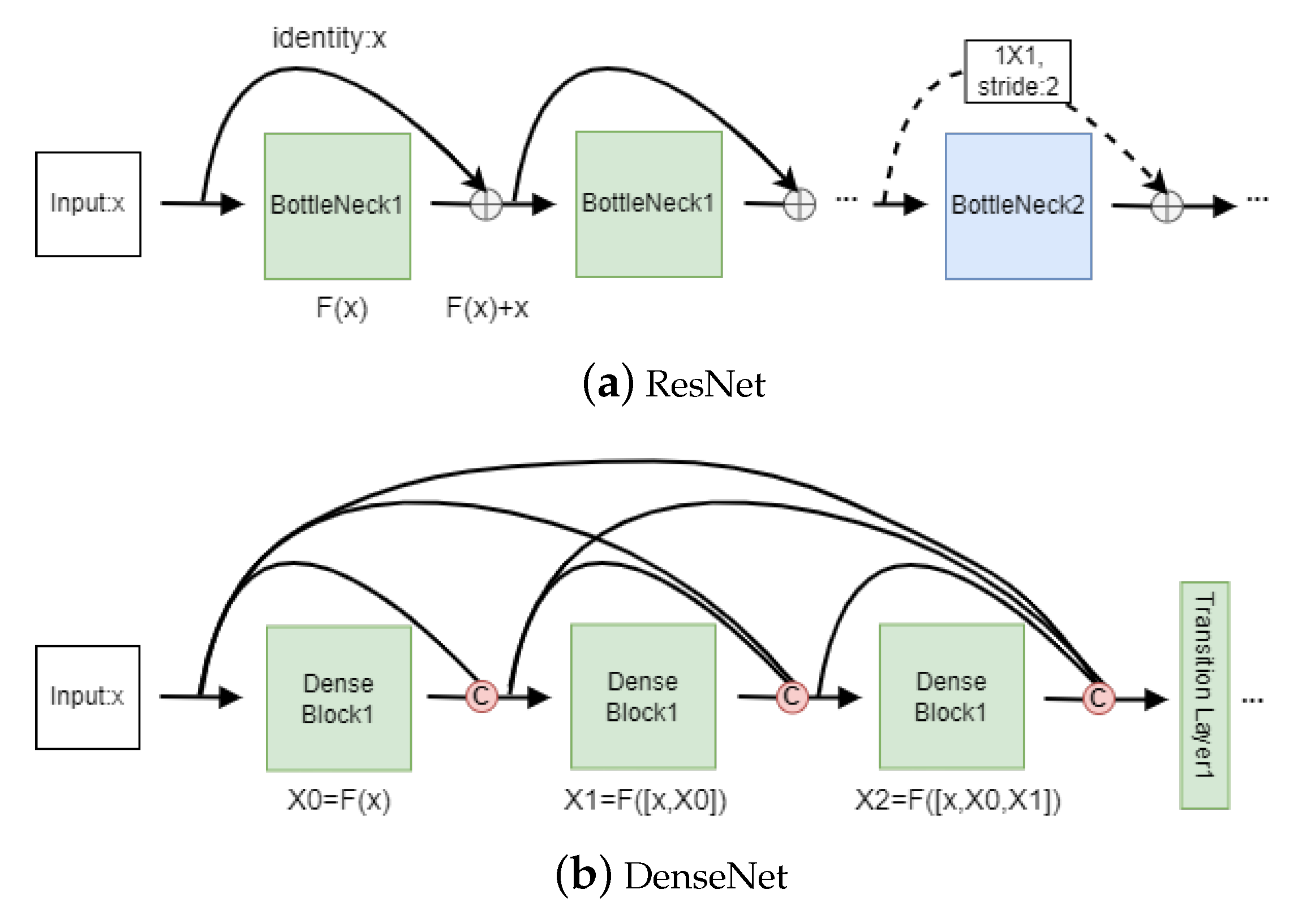
A deep neural network extracts features by stacking several convolutional layers and pooling layers. The features can be enriched with the deepening of the network layer. However, two problems have been found in experiments: one is the vanishing and the exploding gradient, which can be solved by using a batch normalization layer [45]. The other is the degradation problem. Adding more layers will not reduce the training error but instead make it larger. ResNet proposed a residual learning framework to address the degradation problem so that a very deep network can be built. There are two branches in ResNet, as shown in Figure 6a; the first branch extracts features through two or three convolutional layers, and the second branch is called identity mapping and retains the original input. A shortcut connection module performs an element-wise summation between the two branches. When the size of the input and output are the same, the formulation F ( x ) + x can be directly executed (the solid line shortcut in Figure 6a). When the size is different, a 1 × 1 convolution with stride 2 is added to reduce the input size (the dotted line shortcut in Figure 6a). The weight of the first branch can be close to zero if identity mappings are optimal. In this way, the network of layer L + 1 contains more image information than layer L, which ensures a deeper network will not be inferior than its shallower counterpart.
DenseNet is an improvement of ResNet. It is also based on the shortcut connections. The difference is that it adopts a more intensive connection. Figure 6b shows its internal structure; each layer is connected to all of the subsequent layers so that the features of each scale can be reused to maximize the information flow between the layers. Another difference is that it concatenates the multiple feature maps instead of adding all of the elements.
In the encoder part, two networks are designed: one is StrainNetR, which extends ResNet, and the other one is StrainNetD extending DenseNet. Table 3 lists the implementation details of StrainNetR and StrainNetD. StrainNetR consists of four different bottlenecks; each bottleneck includes two 3 × 3 convolutional layers. StrainNetD is implemented by four dense blocks, and each block comprises a 1 × 1 followed by a 3 × 3 convolution with stride 1. 1 × 1 convolution is used to reduce dimensions, making the input of 3 × 3 layer smaller, thus improving the calculation efficiency. The transition layer is responsible for connecting two consecutive dense blocks, which includes a batch normalization layer, a 1 × 1 convolutional layer, and a 2 × 2 pooling layer. After the transition layer, the size of the feature maps will be reduced by half.

2.2.2. Decoder

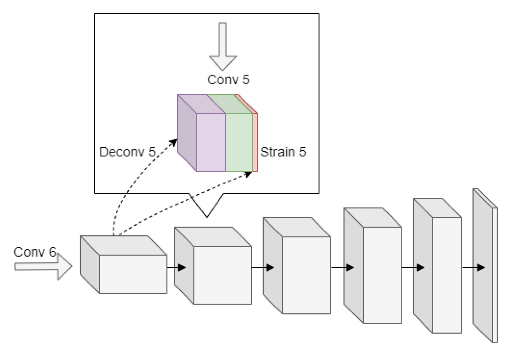
After passing through the encoder, the output size of the feature map is reduced to size 2 × 4 . The decoder will perform a series of up-sampling functions on previous outputs, and each step can expand feature maps twice. The expanding part in FlowNet is slightly modified; the process is shown in Figure 7.
First, the output of the previous layer are expanded through a deconvolution operation (purple cuboid), and an upsampled coarse strain prediction is generated (red cuboid) in a similar way. The corresponding feature maps with the same resolution in the encoder stage (green cuboid) can be reused to preserve the earlier information and prevent the loss of details. These three components are concatenated and used as the input to the next layer. This operation is repeated 5 times to obtain the strain field with the same resolution as the input, instead of bilinear interpolation in FlowNet, which may reduce the quality of results.

3. Results of the Strain Prediction

In this section, the selection of parameters in the training process is introduced first; then, a detailed analysis and comparison of the prediction results is given.

3.1. Training Details

StrainNetR and StrainNetD are both implemented using the PyTorch framework. They are trained on a GPU Nvidia GeForce GTX 1060 6GB. The loss function is the average endpoint error (AEE) between the ground truth (GT) and the predicted strain. The AEE is obtained by calculating the Euclidean distance. In the dataset collected in Section 2.1, cracks propagate in x direction. The strain in y direction is predicted in our experiments because it reflects the occurrence of cracks. G ( x , y ) = ( u T , v T ) and E ( x , y ) = ( u E , v E ) represent the ground truth and the predicted strain, respectively. The loss function of the y-Strain is as follows:
A E E = 1 H W ( v E v T ) 2 ,
where H and W are the height and width of the image, and H W is the total number of pixels. The optimization method is Adam with default parameters b e t a 1 = 0.9 and b e t a 2 = 0.999 . The learning rate is initialized with 1 e 4 and then divided by half at 100 and 150 epochs. A ROI area with the size of 64 × 128 near the melt pool is selected. The total training epoch is 200 rounds. Figure 8 shows the AEE of two networks on the training set and verification set in all epochs. It can be seen from the figures that the convergence of StrainNetD is slightly faster than that of StrainNetR, but this advantage is small. The AEE on the validation set of StrainNetD is finally reduced to 0.0045 , which is 6.3% less than that of StrainNetR.

3.2. Results and Discussion

In this section, the trained models are first verified on two test videos; then, the predicted strains are compared with the ground truth. The real strain fields are generated by calculating the spatial derivatives of the displacement fields obtained from the OpenCV library. The program runs on Intel (R) Xeon (R) CPU E5-2620 v4 2.10 GHz, and it takes about 80 ms to calculate each strain field. The deep learning method can directly predict strain fields from image pairs and benefit from the high performance of the GPU, providing a great advantage in run time. Table 4 shows the comparison of the two models in terms of accuracy and processing time. From the test results, it can be demonstrated that StrainnetR and StrainnetD perform similarly in strain prediction, with AEEs of 0.0439 and 0.0427 , respectively. The number of parameters of StraineNetD is less than half of those of StraineNetR, but the run time of StrainNetD is 5.95 ms per image pair, which is 2.56 ms slower than that of StrateNetR.
This is caused by the different network structures of the two models, due to the use of 1 × 1 convolution, StrainetD has much fewer channel inputs and outputs than StrainetR, so the number of parameters is reduced. However, the feature maps of StrainNetD are reduced to half at the transition layer, as shown in Table 3, which leads to it being twice as large as that of StratinetR. As a result, the number of convolution operations, measured in floating point operations per second (flops), is larger than StratinetR. In addition, DenseNet needs to load all of the previous layers, which will result in frequent memory accesses and thus increase the processing time. In summary, StrainNetD is slightly better than StrainNetR in terms of accuracy, but its prediction time for each image pair is 2 ms longer. Obviously, in real-time prediction applications, StrainNetR is much better due to its higher efficiency.
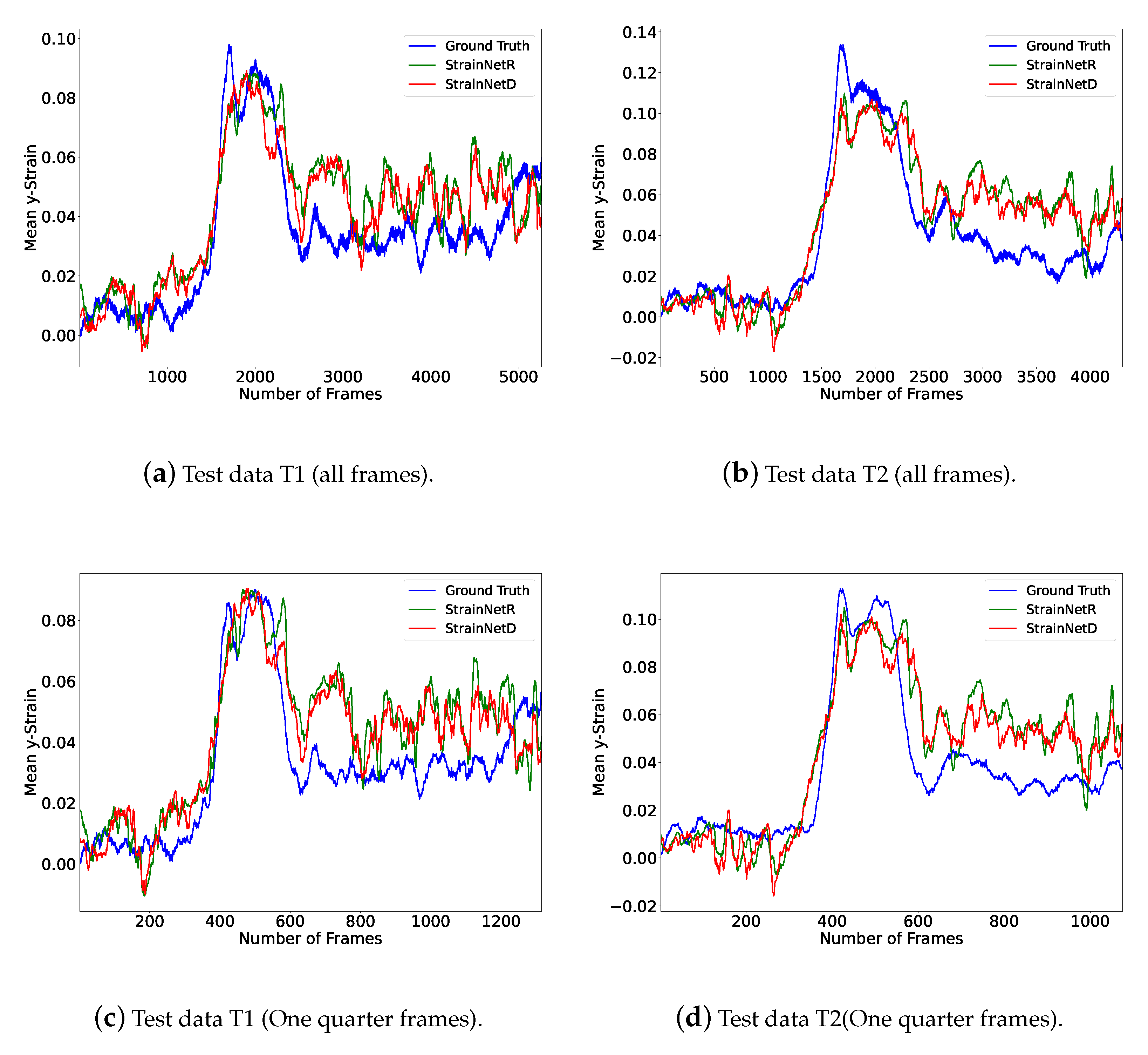
As mentioned in the introduction, cracks start to occur when the strain accumulates and exceeds a critical value. Figure 9 reflects the range of crack initiation and growth; the vertical axis is the average strain in the y direction of each frame. In test data T1, the crack appears at around 1400 frames, and the mean values predicted by StrainNetR and StrainNetD both rise sharply at this time. Although there is still an 0.02 error at the peak value of the strain, the range of crack generation is roughly consistent with the ground truth. Both networks can correctly detect the crack range.
In terms of processing speed, StrainNetR needs 3 ms to process each image pair as listed in Table 4, whereas the image collection speed is about 0.85 ms per frame, which is approximately one quarter of the prediction time. To achieve real-time strain prediction, we can exploit the observation that the displacement between successive frames is very small, and it is sufficient to use one in four frames as input to the networks (ignoring the three frames between them). Figure 9c,d show the strain prediction using the first, fifth, ninth, etc., frame of the video. Reducing the number of analyzed frames to one quarter, the total image-collection time (about 5260 and 4300 frames) remains the same, and the total strain prediction time (about 1315 and 1075 frames) is reduced to one quarter, such that both will are fairly similar; both take in total approximately 4.5 (T1) and 3.6 (T2) seconds. The results show that even if frames are skipped, the strain can still be well predicted, and the predicted crack range is consistent with the results including all of the frames.
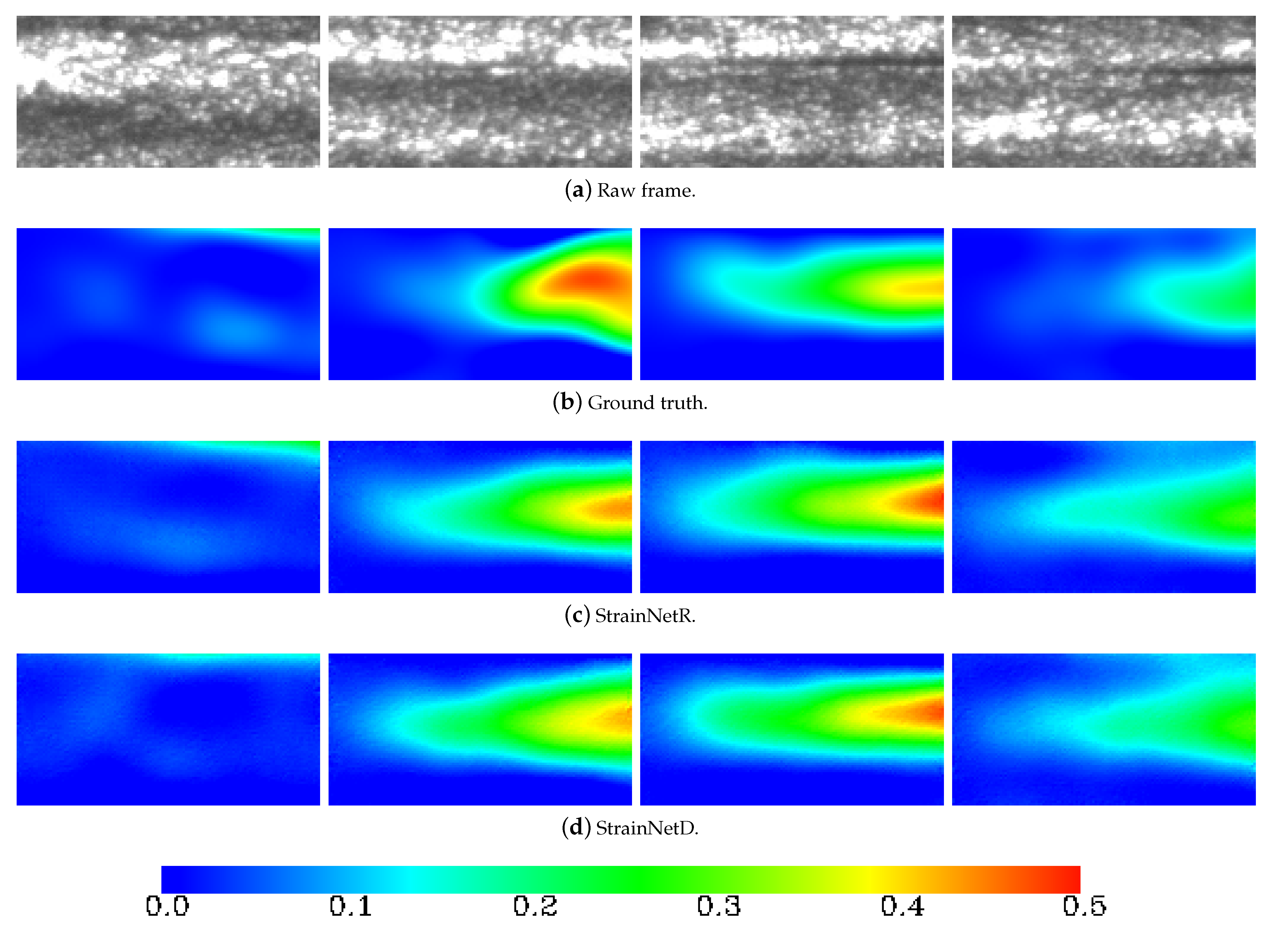
Figure 10 gives some visual examples of predicted strain fields in different stages; the range of the color bar is set according to the strain values of all frames. The first image is the normal state. The second and the third images are stages when a crack starts to occur and propagate. The deformation increases obviously at these stages, and the strain values begin to accumulate. In the last image, the crack begins to shrink and disappears gradually. Although the endpoint error of StrainNetD is a little smaller than that of StrainNetR, this difference is almost invisible in the figure; the two networks give similar predictions during crack initiation and propagation.

4. Conclusions

This paper develops two networks for measuring the strain field in the case of crack occurrence during laser beam welding. The first network StrainNetR uses ResNet as the feature extractor. The second network StrainNetD applies DenseNet, which is an improvement of ResNet with more tight connections. The networks are trained and tested in the real welding dataset collected using the CTW test. The strain prediction results demonstrate that StrainNetD is slightly better than StrainNetR in terms of the AEE. On the other hand, the feature maps of DenseNet are larger, and it requires more memory accesses. The processing time of StrainNetD is nearly twice that of StrainNetR. Compared with traditional methods, both networks can achieve approximately real-time strain prediction within the tolerable error, which enables the timely identification of crack defects in the welding process.
We have shown early results in the prediction of the strain field based on deep learning methods, and further optimization is still necessary. For instance, the data set critically affects the final results. The data in this paper is obtained under several different strain rates. In order to enrich data diversity and improve model robustness, synthetic data are a good choice. Generative adversarial networks (GAN) [46] are a widely used technology to generate desired images. We are considering to use a GAN to generate more weld defect images. On the other hand, the accuracy of strain prediction can be further improved. Transformer networks [47], which have achieved great success in natural language processing, have been gradually explored in computer vision tasks. Next, we plan to combine or replace the CNN model with a transformer model to enhance the accuracy and training efficiency.

Author Contributions

Conceptualization, W.H. and N.B.; Methodology, W.H. and N.B.; Software, W.H. and N.B.; Validation, W.H.; Writing—original draft, W.H. and N.B.; Writing—review & editing, A.G., M.R. and K.W.; Supervision, K.W.; Project administration, N.B. and K.W. All authors have read and agreed to the published version of the manuscript.

Funding

This research was funded by the China Scholarship Council file Nr. 202008610227 and by the Deutsche Forschungsgemeinschaft (DFG, German Research Foundation) project Nr. 434946896 and project Nr. 465316565.

Institutional Review Board Statement

Not applicable.

Informed Consent Statement

Not applicable.

Conflicts of Interest

The funders had no role in the design of the study; in the collection, analyzes, or interpretation of data; in the writing of the manuscript, or in the decision to publish the results.

Abbreviations

The following abbreviations are used in this manuscript:
DICDigital image correlation
CNNConvolutional neural network
CTW test    Controlled tensile weldabilit test
AEEAverage endpoint error
GTGround truth
flopsFloating point operations per second

References

  1. Pellini, W.S. Strain theory of hot tearing. Foundry 1952, 80, 125–133. [Google Scholar]
  2. Apblett, W.; Pellini, W. Factors which influence weld hot cracking. Weld. J. 1954, 33, 83–90. [Google Scholar]
  3. Prokhorov, N. The problem of the strength of metals while solidifying during welding. Svarochnoe Proizv. 1956, 6, 5–11. [Google Scholar]
  4. Prokhorov, N. The Technological Strength of Metals While Crystallizing during Welding; Technical Report, IX-479-65; IIW-Doc, 1965. [Google Scholar]
  5. De Strycker, M.; Lava, P.; Van Paepegem, W.; Schueremans, L.; Debruyne, D. Measuring welding deformations with the digital image correlation technique. Weld. J. 2011, 90, 107S–112S. [Google Scholar]
  6. Shibahara, M.; Onda, T.; Itoh, S.; Masaoka, K. Full-field time-series measurement for three-dimensional deformation under welding. Weld. Int. 2014, 28, 856–864. [Google Scholar] [CrossRef]
  7. Shibahara, M.; Yamaguchi, K.; Onda, T.; Itoh, S.; Masaoka, K. Studies on in-situ full-field measurement for in-plane welding deformation using digital camera. Weld. Int. 2012, 26, 612–620. [Google Scholar] [CrossRef]
  8. Shibahara, M.; Kawamura, E.; Ikushima, K.; Itoh, S.; Mochizuki, M.; Masaoka, K. Development of three-dimensional welding deformation measurement based on stereo imaging technique. Weld. Int. 2012, 27, 920–928. [Google Scholar] [CrossRef]
  9. Chen, J.; Yu, X.; Miller, R.G.; Feng, Z. In situ strain and temperature measurement and modelling during arc welding. Sci. Technol. Weld. Join. 2015, 20, 181–188. [Google Scholar] [CrossRef]
  10. Chen, J.; Feng, Z. Strain and distortion monitoring during arc welding by 3D digital image correlation. Sci. Technol. Weld. Join. 2018, 23, 536–542. [Google Scholar] [CrossRef]
  11. Gollnow, C.; Kannengiesser, T. Hot cracking analysis using in situ digital image correlation technique. Weld. World 2013, 57, 277–284. [Google Scholar] [CrossRef]
  12. Gao, H.; Agarwal, G.; Amirthalingam, M.; Hermans, M.; Richardson, I. Investigation on hot cracking during laser welding by means of experimental and numerical methods. Weld. World 2018, 62, 71–78. [Google Scholar] [CrossRef] [Green Version]
  13. Hagenlocher, C.; Stritt, P.; Weber, R.; Graf, T. Strain signatures associated to the formation of hot cracks during laser beam welding of aluminum alloys. Opt. Lasers Eng. 2018, 100, 131–140. [Google Scholar] [CrossRef]
  14. Baker, S.; Patil, R.; Cheung, K.M.; Matthews, I. Lucas-Kanade 20 Years on: Part 5; Tech. Rep. CMU-RI-TR-04-64; Robotics Institute, Carnegie Mellon University: Pittsburgh, PA, USA, 2004. [Google Scholar]
  15. Pełczyński, P.; Szewczyk, W.; Bieńkowska, M. Single-camera system for measuring paper deformations based on image analysis. Metrol. Meas. Syst. 2021, 28, 509–522. [Google Scholar]
  16. Hoffmann, H.; Vogl, C. Determination of true stress-strain-curves and normal anisotropy in tensile tests with optical strain measurement. CIRP Ann. 2003, 52, 217–220. [Google Scholar] [CrossRef]
  17. Gong, X.; Bansmer, S.; Strobach, C.; Unger, R.; Haupt, M. Deformation measurement of a birdlike airfoil with optical flow and numerical simulation. AIAA J. 2014, 52, 2807–2816. [Google Scholar] [CrossRef]
  18. Bakir, N.; Gumenyuk, A.; Rethmeier, M. Investigation of solidification cracking susceptibility during laser beam welding using an in-situ observation technique. Sci. Technol. Weld. Join. 2018, 23, 234–240. [Google Scholar] [CrossRef]
  19. Bakir, N.; Pavlov, V.; Zavjalov, S.; Volvenko, S.; Gumenyuk, A.; Rethmeier, M. Development of a novel optical measurement technique to investigate the hot cracking susceptibility during laser beam welding. Weld. World 2019, 63, 435–441. [Google Scholar] [CrossRef]
  20. LeCun, Y.; Bottou, L.; Bengio, Y.; Haffner, P. Gradient-based learning applied to document recognition. Proc. IEEE 1998, 86, 2278–2324. [Google Scholar] [CrossRef] [Green Version]
  21. Dosovitskiy, A.; Fischer, P.; Ilg, E.; Hausser, P.; Hazirbas, C.; Golkov, V.; Van Der Smagt, P.; Cremers, D.; Brox, T. Flownet: Learning optical flow with convolutional networks. In Proceedings of the IEEE International Conference on Computer Vision, Santiago, Chile, 7–13 December 2015; pp. 2758–2766. [Google Scholar]
  22. Ilg, E.; Mayer, N.; Saikia, T.; Keuper, M.; Dosovitskiy, A.; Brox, T. Flownet 2.0: Evolution of optical flow estimation with deep networks. In Proceedings of the IEEE Conference on Computer Vision and Pattern Recognition, Honolulu, HI, USA, 21–26 July 2017; pp. 2462–2470. [Google Scholar]
  23. Ranjan, A.; Black, M.J. Optical flow estimation using a spatial pyramid network. In Proceedings of the IEEE Conference on Computer Vision and Pattern Recognition, Honolulu, HI, USA, 21–26 July 2017; pp. 4161–4170. [Google Scholar]
  24. Sun, D.; Yang, X.; Liu, M.Y.; Kautz, J. Pwc-net: Cnns for optical flow using pyramid, warping, and cost volume. In Proceedings of the IEEE Conference on Computer Vision and Pattern Recognition, Salt Lake City, UT, USA, 18–23 June 2018; pp. 8934–8943. [Google Scholar]
  25. Hui, T.W.; Tang, X.; Loy, C.C. Liteflownet: A lightweight convolutional neural network for optical flow estimation. In Proceedings of the IEEE Conference on Computer Vision and Pattern Recognition, Salt Lake City, UT, USA, 18–23 June 2018; pp. 8981–8989. [Google Scholar]
  26. Hur, J.; Roth, S. Iterative residual refinement for joint optical flow and occlusion estimation. In Proceedings of the IEEE/CVF Conference on Computer Vision and Pattern Recognition, Long Beach, CA, USA, 15–20 June 2019; pp. 5754–5763. [Google Scholar]
  27. Yin, Z.; Darrell, T.; Yu, F. Hierarchical discrete distribution decomposition for match density estimation. In Proceedings of the IEEE/CVF Conference on Computer Vision and Pattern Recognition, Long Beach, CA, USA, 15–20 June 2019; pp. 6044–6053. [Google Scholar]
  28. Yang, G.; Ramanan, D. Volumetric correspondence networks for optical flow. Adv. Neural Inf. Process. Syst. 2019, 32, 794–805. [Google Scholar]
  29. Zhao, S.; Sheng, Y.; Dong, Y.; Chang, E.I.; Xu, Y. Maskflownet: Asymmetric feature matching with learnable occlusion mask. In Proceedings of the IEEE/CVF Conference on Computer Vision and Pattern Recognition, Seattle, WA, USA, 13–19 June 2020; pp. 6278–6287. [Google Scholar]
  30. Teed, Z.; Deng, J. Raft: Recurrent all-pairs field transforms for optical flow. In Proceedings of the European Conference on Computer Vision, Glasgow, UK, 23–28 August 2020; Springer: Berlin/Heidelberg, Germany, 2020; pp. 402–419. [Google Scholar]
  31. Sui, X.; Li, S.; Geng, X.; Wu, Y.; Xu, X.; Liu, Y.; Goh, R.; Zhu, H. CRAFT: Cross-Attentional Flow Transformer for Robust Optical Flow. In Proceedings of the IEEE/CVF Conference on Computer Vision and Pattern Recognition, Seattle, WA, USA, 13–19 June 2022; pp. 17602–17611. [Google Scholar]
  32. Xu, H.; Zhang, J.; Cai, J.; Rezatofighi, H.; Tao, D. GMFlow: Learning Optical Flow via Global Matching. In Proceedings of the IEEE/CVF Conference on Computer Vision and Pattern Recognition, New Orleans, LA, USA, 18–24 June 2022; pp. 8121–8130. [Google Scholar]
  33. Zhao, S.; Zhao, L.; Zhang, Z.; Zhou, E.; Metaxas, D. Global Matching with Overlapping Attention for Optical Flow Estimation. In Proceedings of the IEEE/CVF Conference on Computer Vision and Pattern Recognition, New Orleans, LA, USA, 18–24 June 2022; pp. 17592–17601. [Google Scholar]
  34. Hu, L.; Zhao, R.; Ding, Z.; Ma, L.; Shi, B.; Xiong, R.; Huang, T. Optical Flow Estimation for Spiking Camera. In Proceedings of the IEEE/CVF Conference on Computer Vision and Pattern Recognition, New Orleans, LA, USA, 18–24 June 2022; pp. 17844–17853. [Google Scholar]
  35. Rezaie, A.; Achanta, R.; Godio, M.; Beyer, K. Comparison of crack segmentation using digital image correlation measurements and deep learning. Constr. Build. Mater. 2020, 261, 120474. [Google Scholar] [CrossRef]
  36. Boukhtache, S.; Abdelouahab, K.; Berry, F.; Blaysat, B.; Grediac, M.; Sur, F. When deep learning meets digital image correlation. Opt. Lasers Eng. 2021, 136, 106308. [Google Scholar] [CrossRef]
  37. Yang, R.; Li, Y.; Zeng, D.; Guo, P. Deep DIC: Deep learning-based digital image correlation for end-to-end displacement and strain measurement. J. Mater. Process. Technol. 2022, 302, 117474. [Google Scholar] [CrossRef]
  38. Wang, Y.; Zhao, J. DIC-Net: Upgrade the performance of traditional DIC with Hermite dataset and convolution neural network. Opt. Lasers Eng. 2023, 160, 107278. [Google Scholar] [CrossRef]
  39. Wang, Y.; Luo, Q.; Xie, H.; Li, Q.; Sun, G. Digital image correlation (DIC) based damage detection for CFRP laminates by using machine learning based image semantic segmentation. Int. J. Mech. Sci. 2022, 230, 107529. [Google Scholar] [CrossRef]
  40. Bakir, N.; Gumenyuk, A.; Rethmeier, M. Numerical simulation of solidification crack formation during laser beam welding of austenitic stainless steels under external load. Weld. World 2016, 60, 1001–1008. [Google Scholar] [CrossRef]
  41. Ronneberger, O.; Fischer, P.; Brox, T. U-net: Convolutional networks for biomedical image segmentation. In Proceedings of the International Conference on Medical Image Computing and Computer-Assisted Intervention, Munich, Germany, 5–9 October 2015; Springer: Berlin/Heidelberg, Germany, 2015; pp. 234–241. [Google Scholar]
  42. He, K.; Zhang, X.; Ren, S.; Sun, J. Deep residual learning for image recognition. In Proceedings of the IEEE Conference on Computer Vision and Pattern Recognition, Las Vegas, NV, USA, 27–30 June 2016; pp. 770–778. [Google Scholar]
  43. Huang, G.; Liu, Z.; Van Der Maaten, L.; Weinberger, K.Q. Densely connected convolutional networks. In Proceedings of the IEEE Conference on Computer Vision and Pattern Recognition, Honolulu, HI, USA, 21–26 July 2017; pp. 4700–4708. [Google Scholar]
  44. Lucas, B.D.; Kanade, T. An iterative image registration technique with an application to stereo vision. In Proceedings of the IJCAI’81: 7th International Joint Conference on Artificial Intelligence, Vancouver, BC, Canada, 24 August 1981; Volume 81. [Google Scholar]
  45. Ioffe, S.; Szegedy, C. Batch normalization: Accelerating deep network training by reducing internal covariate shift. In Proceedings of the International Conference on Machine Learning, Lille, France, 7–9 July 2015; pp. 448–456. [Google Scholar]
  46. Goodfellow, I.; Pouget-Abadie, J.; Mirza, M.; Xu, B.; Warde-Farley, D.; Ozair, S.; Courville, A.; Bengio, Y. Generative adversarial networks. Commun. ACM 2020, 63, 139–144. [Google Scholar] [CrossRef]
  47. Vaswani, A.; Shazeer, N.; Parmar, N.; Uszkoreit, J.; Jones, L.; Gomez, A.N.; Kaiser, Ł.; Polosukhin, I. Attention is all you need. Adv. Neural Inf. Process. Syst. 2017, 30, 5998–6008. [Google Scholar]
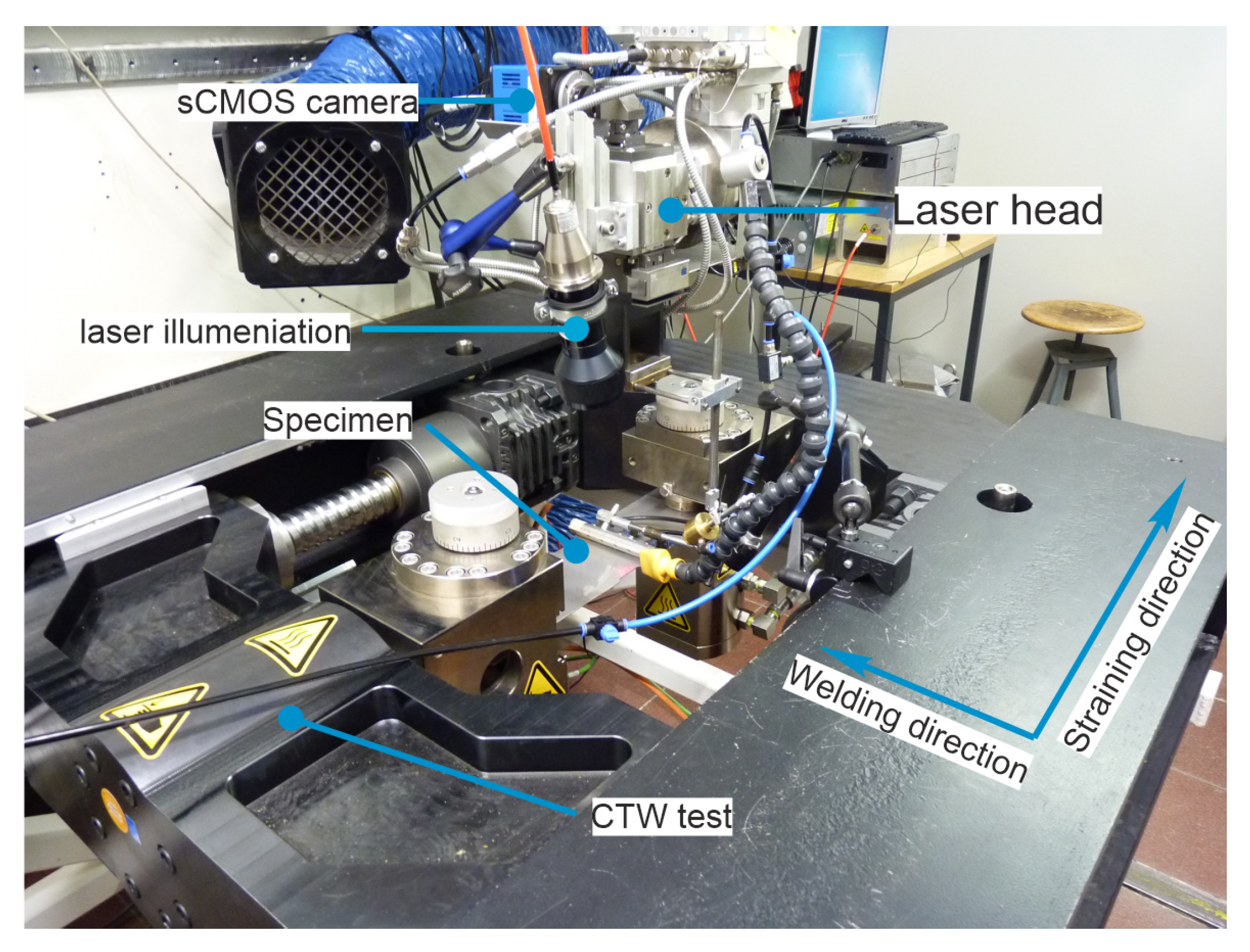
Figure 1. The experimental setup of the welding under external strain using CTW test.
Applsci 13 02930 g001
Figure 2. Schematic representation of the CTW test procedure during laser beam welding.
Applsci 13 02930 g002
Figure 3. Image was taken during welding and shows the formation of a solidification crack.
Applsci 13 02930 g003
Figure 4. Strain distribution and three moments for the test data T2 (a) before the straining starts, (b) at the crack initiation moment, and (c) after the initiation and during the propagation of the crack. (d) Average strain history for the selected ROI over the frames.
Applsci 13 02930 g004
Figure 5. Structure of the strain prediction network.
Applsci 13 02930 g005
Figure 6. Internal architectures of ResNet and DenseNet.
Applsci 13 02930 g006
Figure 7. The decoder recovers the feature maps to predict the strain field.
Applsci 13 02930 g007
Figure 8. Average endpoint error (AEE) in training and validation stages.
Applsci 13 02930 g008
Figure 9. Average y-Strain value per frame.
Applsci 13 02930 g009
Figure 10. Visual examples of predicted strain fields.
Applsci 13 02930 g010
Table 1. Chemical composition (in wt-%) of the investigated material.
CCrNiMnMoSiPSNFe
0.0316.9510.571.362.280.390.040.0040.019Bal.
Table 2. Details of train/validation set (TD1–TD4) and test set (T1 and T2).
Train/Validation SetCTW Strain in %CTW Strain Rate in s 1 Data Quantity (Images)
TD1745030
TD2745080
TD3765000
TD4765000
Test SetCTW Strain in %CTW Strain Rate in s 1 Data Quantity (Images)
T1785260
T2784300
Table 3. Configuration of StrainNetR and StrainNetD.
StrainNetRStrainNetD
Layer NameKernel SizeOutput SizeLayer NameKernel SizeOutput Size
Convolution 3 × 3 , 32 32 × 64 Convolution 3 × 3 , 32 32 × 64
Bottleneck1 3 × 3 , 64 3 × 3 , 64 × 2 16 × 32 Dense Block1 1 × 1 , C o n v 3 × 3 , C o n v × 3 32 × 64
Transition Layer1 1 × 1 , 64 2 × 2 , P o o l 16 × 32
Bottleneck2 3 × 3 , 128 3 × 3 , 128 × 2 8 × 16 Dense Block2 1 × 1 , C o n v 3 × 3 , C o n v × 6 16 × 32
Transition Layer2 1 × 1 , 128 2 × 2 , P o o l 8 × 16
Bottleneck3 3 × 3 , 256 3 × 3 , 256 × 2 4 × 8 Dense Block3 1 × 1 , C o n v 3 × 3 , C o n v × 12 8 × 16
Transition Layer3 1 × 1 , 256 2 × 2 , P o o l 4 × 8
Bottleneck4 3 × 3 , 512 3 × 3 , 512 × 2 2 × 4 Dense Block4 1 × 1 , C o n v 3 × 3 , C o n v × 8 4 × 8
Pooling 2 × 2 , P o o l 2 × 4
Table 4. Average endpoint errors and run times of the test set.
ModelParameters (M)Flops (G)AEETime (ms)
StrainNetR1.470.880.04393.39
StrainNetD0.571.270.04275.95
Disclaimer/Publisher’s Note: The statements, opinions and data contained in all publications are solely those of the individual author(s) and contributor(s) and not of MDPI and/or the editor(s). MDPI and/or the editor(s) disclaim responsibility for any injury to people or property resulting from any ideas, methods, instructions or products referred to in the content.