Time-Frequency Feature-Based Seismic Response Prediction Neural Network Model for Building Structures

Abstract

Currently, machine learning techniques are widely used in structural seismic response studies. The developed network models for various types of seismic response provide new ways to analyse seismic hazards. However, it is not easy to balance the applicability of the input, accuracy, and computational efficiency for existing network models. In this paper, a neural network model containing an efficient self-adaptive feature extraction module (AFEM) is designed. It can recognize time-frequency features from ground motion (GM) inputs for structural seismic response prediction tasks while considering the model’s computational accuracy and computational cost. The self-adaptive feature extraction module is constructed based on the MFCCs feature extraction process in NLP. AFEM recognizes time-frequency features closely related to structures’ behaviour and response under dynamic loads. Taking the seismic response prediction of a typical building as the target task, the neural network configuration, including a baseline model $M_0$ and three comparison models ($M_1$, $M_2$, and $M_3$) with AFEM, is systematically analysed. The results demonstrate that the proposed $M_1$ model with initial AFEM, the $M_2$ model with combined amplitude and phase features, and the $M_3$ model with a complex-valued network are more adaptable than the baseline model to the target task. The extracted amplitude and phase features by the $M_3$ model’s AFEM significantly improve model validation accuracy by 8.6% while reducing computation time by 11.4%. It could provide the basis for future research on regional earthquake damage intelligence assessment systems.

1. Introduction

Seismic (especially strong) hazards have long been a severe threat to public life and well-being [1], which are highly sudden, cause large-scale destruction, are widely influenced, and firmly interlocked. Earthquakes cause catastrophic casualties and significant economic losses. Therefore, research on seismic hazards [2,3,4,5] has continued, where structural seismic response prediction (or assessment) are hot areas. Whether vulnerability analysis and capability spectrum (CSM) method studies [6,7,8] or structural seismic response studies based on NLTHA [9,10,11], an analysis is carried out by constructing a hazard-to-damage mapping model. As a result, the method of using neural networks for analysis was successfully introduced [12,13] into the field of seismic hazard research. For example, O.R. et al. [14] combined an autoregressive (AR) model with an artificial neural net (ANN) [15] to predict structural responses and detect damage by using long time series of acceleration data as initial inputs to the hybrid model. C.S. Huang et al. [16] used the previous and current steps of ground motion (GM) acceleration as input signals and constructed a backpropagation neural network (BPNN) model to recognize the dynamic properties of buildings and assess post-earthquake structural damage. However, the calculation cost for various models that use this input must be considered due to the inherent complexity of GM data (the long time series acceleration data). For example, D.M. Sahoo. et al. [17] proposed a model for predicting the seismic response of multi-degrees-of-freedom structures using functionally linked neural networks (FLNN). To reduce the computational cost, the Chebyshev and Legendre polynomials were introduced in the model to process the GM data. Xu Y et al. [18] created a real-time framework for assessing regional structural damage. This study used a long short-term memory (LSTM) neural network architecture with adjusted truncated GM data as the input to improve the stability of network training and reduce the calculation time.

On the other hand, researchers used the main features of GM data extracted by hand as the input of the neural network for building the analytical model. O.R. de Lautour et al. [19] used the ANNs technique to create a mapping between structural and ground motion characteristics with damage indices. The input part of this model adopted some main parameters that can represent ground motion characteristics: peak ground acceleration (PGA), peak ground velocity (PGV), peak ground displacement (PGD), duration, and dominant frequency, supplemented by some building structure parameters; the output part was an index that describes the degree of damage. K. Morfidis. et al. [20] proposed a model of ANNs that can predict the damage state of R/C buildings. For the selection of network inputs, they considered the results of a previous study on the correlation between ground motion intensity measures (IMs) and structural seismic dynamic response [21]. Specifically, 14 main seismic parameters and their combinations are extracted from recorded GM data and combined with additional building structure parameters, which generate the inputs for ANNs. Oh B.K. et al. [22] developed a neural network that can act as a proxy for the relationship between GM features and structural seismic responses. They extracted GM features from artificial earthquakes: significant duration, mean and predominant period, PGA, and resonance area.

Essentially, GM data is a kind of ground motion signal that is captured through sensors, etc. It objectively reflects the real situation and accordingly does not have comparatively strong task information, and the density of task information may be very low. So, GM data in the above study mainly needs to be ‘purified’ and then fed to the neural network model to meet the task requirements, and this refinement is mainly done by hand. Nevertheless, such hand-crafted features may face the following challenges in use. Namely, (a) an accurate description of the seismic response needs detailed consideration for both time domain features and frequency domain features of earthquakes. Furthermore, a hand-crafted GM feature may not always be the best. (b) Multiple factors (e.g., target task, target accuracy, etc.) must be considered when producing GM features by hand. It is also a problem to balance between feature production efficiency and the accuracy and calculation cost of the task model. Furthermore, the damage caused by earthquakes to building structures is catastrophic. Researchers from different countries have studied various aspects of vibration control problems under seismic effects [23,24], such as active and semi-active vibration control of important building structures. Intelligent control strategies, whose core technology is to quickly capture the model parameters of controlled objects with known responses and predict the structural response at unknown moments in real time and accurately [25,26], have more or less various defects, so the prediction of a building’s structural response under ground shaking is also a very critical and challenging topic in vibration control.

Considering the above observations and perspectives, designing a method that gives a suitable GM feature representation for the task at hand seems necessary, combining GM feature extraction with the target task and self-adaptively retaining the ground motion features that match the task at hand. In addition, it should also be available to improve the efficiency of the task when it is used, and achieve a balance between the seismic damage prediction method’s evaluation accuracy and computational efficiency.

Deep learning (DL) [27] techniques are one of the ways to achieve this goal. Indeed, Recurrent neural network (RNN) [28] architectures in DL have already been used in earthquake engineering. For example, seismic waveform classification by RNN [29,30], earthquake location and time prediction [31], seismic trend prediction using LSTM [32], response prediction for buildings [33,34,35,36], etc. Moreover, natural language is an information carrier created by humans for storing knowledge and communicating. Investigators [37] have created many successful natural language processing techniques to enable machines to obtain information in language accurately. Several methods have recently been applied in seismic/vibration feature extraction processes [38,39,40,41]. Nevertheless, these feature designs are separate from the task network model; thus, the designed features may not be the best fit for the target task. Other than that, no GM feature recognition method is self-adaptive to the target task.

This paper presents a time-frequency feature-based seismic response prediction model for building structures, containing two parts: an adaptive feature extraction module (AFEM) and a classification module. The proposed model uses a neural network configuration to predict the seismic state of building structures by combining AFEM with a classification network to adaptively extract time-frequency features, using ground motion records as the input that are closely related to the behaviour and response of the structure under dynamic loads. The model can also be directly embedded into a machine learning-based intelligent assessment method for efficient prediction of regional structural earthquake damage. In addition, the estimation results from neural networks with different weight constraints, different initialization methods, and different network structures and their computational costs are discussed. The study is organized as follows. In Section 2, the proposed seismic damage prediction model is illustrated in detail, including the dataset and the construction of the proposed network. Then, in Section 3, the details of parameter tuning for the proposed models are analysed and discussed, and the prediction performance of each model is presented. Finally, conclusions are provided in Section 4.

2. Proposed Seismic Damage Prediction Model for a Building Structure

The proposed seismic damage prediction model for a building structure includes time-frequency feature extraction and a classification network module. It establishes the relationship between ground motion data and the seismic response of a structure to the earthquake based on the time-frequency feature. Before creating the dataset for such a model, GM data and the structural responses of a building structure to the GM need to be obtained. In this study, historical seismic data obtained from the open database is used for neural network training. However, some preprocessing is performed before inputting the data into the network, including amplitude adjustment, frequency adjustment, and time-holding adjustment. The damage response states of a target structure to ground motion are obtained by conducting a structural dynamic response analysis of the building and extracting seismic responses from the results. When the preprocessed seismic wave data and seismic damage states obtained from the dynamic analysis are obtained, these parameters are used as input and output data sets, respectively, to perform training and generate a seismic prediction model corresponding to the target structure. In the event of a future earthquake, the constructed model is used to predict the seismic damage of a target structure by simply inputting GM data.

2.1. Generation Data Labels

In creating high-quality labels for the structural seismic response, two factors must be considered: the structural seismic response model and seismic damage index selection.

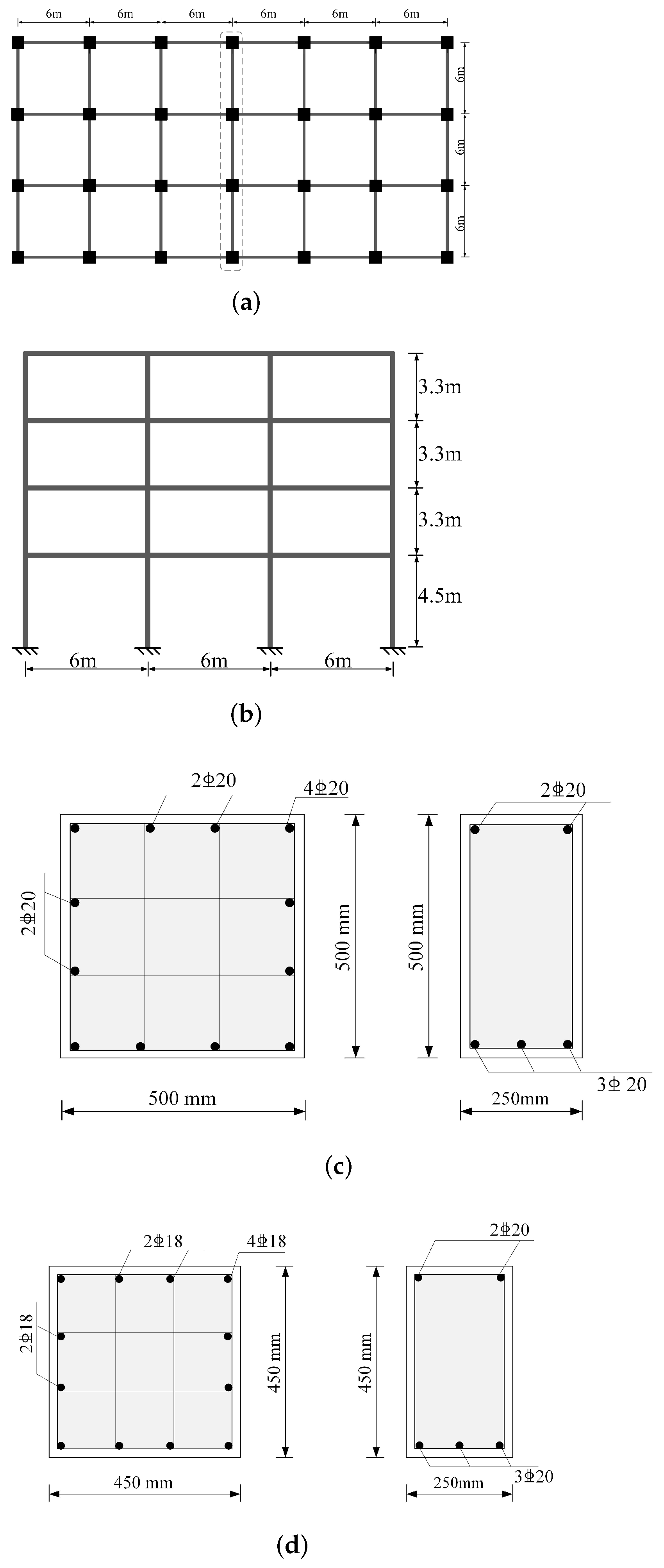
2.1.1. Dynamic Response Analysis Model for the Target Structure

The seismic response of the structure is obtained from the numerical simulation of a planar-reinforced concrete moment-resisting frame (RCMRF). As shown in Figure 1a, the building model is a four-storey, three-span office building in Nansha District, Guangzhou City. The load designed by the code [42], dead load and live load on the 1–3 floors are $5.0$ kN/m${}^2$ and $2.0$ kN/m${}^2$, respectively, and the dead load and live load on the roof are $6.0$ kN/m${}^2$ and $0.5$ kN/m${}^2$, respectively. The sizes and reinforcement of beams and columns from the bottom and standard floor are shown in Figure 1c,d, respectively. In addition, the distance for both horizontal directions between the columns is $6.0$ m. The floor level of the first floor is $4.5$ m, and the remaining floors are $3.3$ m. The columns, beams, and slabs are made of C30 concrete and HRB400 steel. The RC slab and protection layer thicknesses are 120 mm and 40 mm, respectively. The code for the seismic design of buildings is considered [43,44], and the main design parameters include the following: seismic intensity (7), the basic design peak ground acceleration of $0.1$ g (10% in 50 years), site class II, and seismic design group (2). In this paper, the intermediate frame shown in Figure 1b is selected for seismic analysis using OpenSees [45] finite element analysis software. Additionally, there is more information about this model in the study [46]. The effectiveness of the model has been proven in studies [47].

2.1.2. Definition of Structural Damage State

The maximum inter-story displacement ratio (MIDR) is used as a basis for the damage classification of the target structure [48,49,50]. It is extracted from the results of the dynamic response analysis carried out on the structural model. In this paper, the damage state for a building is defined in five different levels: no damage (MIDR $\le 1/550$), minor damage ($1/550<$ MIDR $\le 1\%$), moderate damage ($1\%<$ MIDR $\le 2\%$), extensive damage ($2\%<$ MIDR $\le 4\%$), and complete damage (MIDR $>4\%$). Other damage level definitions can also be accommodated through the proposed model.

2.2. Ground Motion Dataset

Currently, there are a few databases that record ground motion [51,52,53,54]. In this study, 8079 and 1590 records are extracted from the PEER and K-NET databases, respectively. The distribution of the ground motion records according to their PGA, moment magnitude and epicentral distance are shown in Figure 2. Figure 3a shows one of the ground motion records, and Figure 3b shows the Log Mel-spectrum feature and MFCCs hand-crafted from it. Here, more attention is focused on those seismic waves that cause a significant seismic response in the structure, so weaker ground motion records (e.g., PGA $<0.15$m/s${}^2$) are not selected in this study. Moreover, the inherent scarcity of high-amplitude motion could result in a tiny number of destructive earthquakes in the ground motion record, making the dataset highly inhomogeneous and increasing the adverse effects of network training. Therefore, the obtained GM history records are adjusted in amplitude. The frequency adjustment and duration time adjustment methods are used to process the data, which can reduce the network input dimension while catching the main feature of ground motion. Studies [18,38] have shown the rationality and effectiveness of these methods.

2.2.1. Training Set (Validation Set)

The GM data from the PEER database is selected as the training set, while $5\%$ is used as the validation set, and samples are preprocessed through the following three steps. (a) Amplitude adjustment. As shown in Figure 4, the distribution of samples in the GM dataset (before adjustment) is highly non-uniform, with a low percentage of strong earthquakes and nearly $92.72\%$ of “None” and “slight” samples. Therefore, the same strategy as in the codes [44,50] is used to “scale” the natural ground motion data using scale factors of $1.0$, $2.0$, $3.0$, and $4.0$ multiplied by the acceleration records. Richer data is obtained after adjustment, where the percentage of extensive damage samples increased by a factor of $4.36$. Of course, other methods (e.g., random simulation [55], etc.) are also suitable; (b) Frequency adjustment. Samples are down-sampled to 100 Hz using a fixed interval screening method so that all samples are at the same frequency. As well, according to the Nesbitt theorem [56], the maximum analysis frequency is set at 50 Hz in AFEM, which is enough for most earthquake engineering applications [57]; (c) Duration adjustment. As shown in Figure 3a, we adjust the duration of the ground motion data to a uniform size (the minimum is $30.73$ s) by good clipping or zero padding [50]. In addition, sample statistics show that energy in the intercepted data accounts for an average of $90.51\%$ of the original data energy. So, samples retain most of the energy for the ground motion signal.

Finally, 32,304 samples are obtained after preprocessing, which contain 30,688 training samples and 1616 validation samples.

2.2.2. Testing Set

A test dataset is built with GM data obtained from K-NET to prevent data leakage. After frequency and duration adjustment, 1590 samples are obtained. Whether in the training or test set, sample labels are obtained before frequency and duration adjustment, which gives a one-to-one correspondence between the label and the seismic response. It helps to avoid systematic errors accused by the data during frequency and duration adjustment.

2.3. Neural Network Configurations

This study proposes four neural network configurations for seismic damage prediction, including a baseline network. The prediction performances of these configurations are comparatively evaluated in Section 3. Besides the baseline network, each neural network configuration contains an adaptive frequency feature extraction network module and a classification network module. The effects of the network parameter settings for both modules are also analysed.

2.3.1. Model $M_0$

The baseline network $M_0$ model: An NLP approach (MFCCs [58]) is used for the hand-crafted feature. It is designed with inspiration from how humans perceive speech signals [59] and physiological evidence directed to the human ear structure. The same features are used for vibration signals [41], which achieve good results. Figure 3b shows the features we extracted by hand, and the specific steps are also shown in Figure 5-$M_0$, where the samples are pre-emphasized, framed (frame length is $0.05$ s, frameshift is $0.03$ s), windowed (hann window), and then the time domain samples are converted to frequency domain samples by fast Fourier transformation (FFT) [60]. Following, a 40-dimensional Mel-filter set is applied to map the frequency domain samples to Mel-scale, which is calculated as follows:

$$F\left(mel\right)=2595\times log10[1+\frac{f}{700}]$$

(1)

here, f is the signal frequency, and F is the Mel-scale. The sample is transformed into a linear Mel-spectrum. Then, the log Mel-spectrum is obtained by non-linear activation log, and a signal with a lower amplitude and frequency is amplified in this way. The discrete cosine transform (DCT) is the final step of MFCCs, which aims to compress data dimensionality, and it is calculated as follows:

$$C\left(n\right)=\sum _{m=1}^{M}S\left(m\right)cos\left(\frac{n(m-1/2)\pi }{M}\right)$$

(2)

where $S\left(m\right)$ is the log Mel-spectrum, m is the number of Mel-filters, and n is the DCT transform corresponding to m. Moreover, short-time energy [61] is added to enhance the time-domain features of samples. In addition, the classification module of the $M_0$ network is composed of some gated recurrent unit (GRU) [62,63] layers and fully connected layers. It outputs the probability that five damage states occur. In Section 3, the effect of its parameter settings is also analysed.

2.3.2. Model $M_1$

$M_1$: The time-frequency feature extraction process is implemented by an adaptive feature extraction module (AFEM), and the same classification network module as the baseline network is used. However, rather than the MFCC extraction process, AFEM automatically generates time-frequency features that are best suited to the target task with a data-driven approach, and features are learned in the frequency domain. Compared to data-driven feature learning methods conducted directly from time-domain waveforms [64,65,66], frequency-domain learning does not need to consider the complexity of time-domain convolution and additional parameter tuning. At the same time, the Fourier transforms without any parameters would be simpler and improve calculation efficiency [67]. On the other hand, a similar method exists in the study of NLP [68,69,70]. However, we extend the structure and different parameter settings for seismic wave data. Specifically, as shown in Figure 5-$M_1$, the preprocessed GM dataset is used to input AFEM. A sample is split into multiple segments along the time dimension after the short-time Fourier transform (STFT), and the step is similar to frame splitting, windowing, and the FFT used in extracting MFCCs. Here, the same parameters are chosen: a frame length of $0.05$ s and a frameshift of $0.03$ s. Next, the data flows through two normalized transformation layers (Norm-1 and Norm-2). The first normalization layer is used to transform data from the complex domain to the real domain to obtain the power spectrum (or amplitude spectrum). The first normalization layer uses the squared (or absolute) value. The second normalization layer removes the distribution differences between layers and improves the training stability and model performance. A detailed discussion of the parameter settings is given in Section 3.3.

Then, a linear transform layer that can be learned is used to process the samples, and its weight matrix is similar to filters in MFCCs, where each row represents an n-dimensional filter. Benefiting from the idea of sharing neural network weights [71], which allows the weights to be replicated at least once over a small frequency range, the final learned frequency features will be more prosperous and more adapted to the target task.

The data is fed to the classification module through a non-linear activation layer. A power function or a logarithmic function can be chosen for the activation layer function, which has different contributions to the AFEM. The detailed analysis is presented in Section 3.3.4. Moreover, DCT and short-time energy connections are also added to AFEM (Figure 5-$M_1$) for easy comparison with the baseline model ($M_0$).

Note that although the feature learning process here is similar to MFCCs, it can be combined with other parts of the neural network to learn features through the objective function for the task at hand instead of being designed in advance. Furthermore, we believe that this module, with a slight transformation, can be combined with other FFT transform-based feature extraction methods (i.e., LFCC [72], BFCC [73], etc.) that provide multiple feature choices for different types of tasks using GM data as the input.

2.3.3. Model $M_2$

$M_2$ is formed by combining two $M_1$ models with the same inputs. As shown in Figure 5-$M_2$, samples are transformed by the STFT layer to generate two groups of features: ($\left|S\left(e^{jw}\right)\right|$) amplitude and phase ($\angle S\left(e^{jw}\right)$), which are normalized (i.e., Norm 2 in Figure 5-$M_2$) and entered into linear transformation layers ①/② to extract features, followed by non-linear activation and joining short-time energy after DCT transformation that finally produces two kinds of features. It can be seen that the phase feature extraction process is consistent with the amplitude feature extraction. Moreover, $M_2$ uses the same initialization weight in the linear transformation layer as the $M_1$ model.

2.3.4. Model $M_3$

In non-stationary physical data, the phase information can stabilize the training and improve the generalization ability of the neural network [74]. Another way to effectively combine amplitude and phase is complex, namely real and imaginary parts. In this regard, a deep complex network is advantageous, providing the benefit of explicitly modelling in the phase space for physical systems and has been used with good results in studies, such as synthetic aperture radar (SAR) image processing [75].

$M_3$ (Figure 5-$M_3$): The first half of the AFEM in our setting uses a complex network. Data are converted to a real-valued network after a linear transformation layer. Here, note that the BN and LN of complex arrays are not normalized in the same way as real-valued arrays. The study [76] indicates that shifting and scaling the complex array to a distribution with mean 0 and variance 1 is not enough, and the resulting sample space is elliptical and may have high eccentricity. Therefore, BN and LN of complex arrays are achieved by replacing the normalization with a whitening operation of a 2D vector, calculated as follows:

$$\tilde{x}=V^{-\frac{1}{2}}(x-\mathbb{E}\left[x\right])$$

(3)

where x is the sample data, V is its $2\times 2$ covariance matrix, and the covariance matrix is calculated as follows:

$$\begin{array}{ccc}\hfill V=& \left[\begin{array}{cc}{V}_{rr}& V_{ri}\\ V_{ir}& V_{ii}\end{array}\right]=\left[\begin{array}{cc}Cov(\Re \left\{x\right\},\Re \left\{x\right\})& Cov(\Re \left\{x\right\},\Im \left\{x\right\})\\ Cov(\Im \left\{x\right\},\Re \left\{x\right\})& Cov(\Im \left\{x\right\},\Im \left\{x\right\})\end{array}\right]\hfill & \hfill \end{array}$$

(4)

here, the standard normal complex distribution is achieved by transforming the data to be 0 as the centre and multiplying it by the square root of the variance for both components. Furthermore, in the linear transformation layer of the complex array, the following equation is used:

$$\begin{array}{ccc}\hfill Y=& \left\{\begin{array}{c}\Re \left\{Y\right\}\\ \Im \left\{Y\right\}\end{array}\right\}=\left[\begin{array}{cc}{W}_{\Re }& -W_{\Im }\\ W_{\Im }& W_{\Re }\end{array}\right]\times \left[\begin{array}{c}{X}_{\Re }\\ X_{\Im }\end{array}\right]\hfill & \hfill \end{array}$$

(5)

$$\begin{array}{ccc}\hfill & \left|Y\right|={\left[\Re {\left\{Y\right\}}^2+\Im {\left\{Y\right\}}^2\right]}^{\frac{1}{2}}\hfill & \hfill \end{array}$$

(6)

The conversion from a complex domain to a real domain is completed by Equation (6). Here, since the complex operation in AFEM does not contain loss and activation functions, the weights can be learned by back propagation. The program is completed in the Tensorflow$2.2$ [77] framework using the above calculation.

2.4. Calculation Platform and Network Training Setup

All calculation operations in this study are performed on a computer that is equipped with an AMD Ryzen Threadripper $2950X$ at $3.5$ GHz and an NVIDIA RTX 3080 Ti (12 GB) graphics card. For software, the operating platform is Windows 10, and the main program is built using Python $3.7$. In addition, the Tensorflow [77] framework is selected to build a deep neural network model and used for training and testing.

The output of the model is a label corresponding to the input, and the loss function is set with categorical cross-entropy. Adam [78] is used for optimization during the training period, and batch size is determined according to calculation resources. Unless otherwise indicated, the batch size is set to 128 for this study. Furthermore, to account for the instability of the model optimization process, three Monte Carlo simulations are carried out independently for each network configuration.

3. Analysis and Discussion

In this section, the proposed seismic damage prediction model is applied to a four-storey office reinforced-concrete building (Figure 1). The four models in Section 2.3 are used to predict structural seismic damage and evaluate the prediction model’s performance. The parameter settings of those models are analysed and discussed.

3.1. Study on GRU Parameter Settings

The effects of parameter settings for the target task (seismic response prediction of structural) model are systematically analysed using the $M_0$ model in this subsection. The inputs to the model are MFCCs (in Section 2.3.1 with a size of $1024\times 13$, where the first dimension is the short-time energy and the other dimensions are MFCCs with 12 coefficients.

3.1.1. Network Structure

The “number of cells in the hidden layer” and “number of hidden layers” are key parameters that influence the network’s structure. As shown in

Table 1. Network configurations, accuracies (validation set), and the number of parameters on the graph.

No.	Number of Layers	Number of Cells in Each Layer	Accuracy $(\%)$	Parameters on Graph
1	1	32	86.94	4581
2	1	64	87.19	15,301
3	1	128	87.38	55,173
4	1	256	87.62	208,645
5	2	32	87.54	10,917
6	2	64	87.69	40,261
7	2	128	88.06	154,245
8	2	256	87.44	603,397
9	3	32	87.62	17,253
10	3	64	87.37	65,221
11	3	128	87.53	253,317
12	3	256	87.27	998,149
13	4	32	88.30	23,589
14	4	64	87.56	90,181
15	4	128	87.19	352,389

Note: Values of other hyperparameters are as follows: Learning rate = 0.001; batch size = 128; maximum iterations = 100; dropout ratio = 0.3 for the output layer, 0 for the input and hidden layers.

, 15 models are trained to analyse the network structure parameters. The accuracy of the listed models is an average value obtained on the validation set after three Monte Carlo training runs for each network. The last column shows the trainable parameters of each network, which can be used as an index of network complexity when accuracies are calculated on the same platform. In addition, four additional GRU networks are trained, and the inputs to these networks are GM data (long time series data) without having the features extracted by hand, similar to the inputs of the study [18]. However, our inputs are in 3074 dimensions, and the network structure parameters are the same as networks 1, 5, 9, and 13 in Table 1.

Although a marginal error may theoretically be introduced during data preprocessing, MFCCs accurately reflect the main features of ground motion and provide good Mo model performance. Therefore, we use it as a baseline to compare and analyse whether the features extracted by AFEM are more suitable for this model. In addition, compared with the model that uses truncated long time series as the input, the MFCC features lead to an average improvement of $5.1\%$ in model validation accuracy and a $60.4\%$ reduction in training time, which are significant improvements in both. However, it still does not prove that the hand-crafted features are the most suitable features for the target task (structural seismic response prediction). After all, MFCCs correspond to human ear structures, not building structures.

On the other hand, better performance of the task network can be achieved by balancing the number of hidden layers, the number of cells in the hidden layers, and the network complexity, as shown in Table 1. Here, models 4, 6, 7, 9, and 13 have fewer parameters and a higher verification accuracy.

3.1.2. Sensitivity Studies on the Hyperparameters

Apart from the network structure, the hyper-parameters of the proposed network (e.g., dropout ratio and learning rate) have an important influence on the model’s performance [79].

3.1.2.1. Dropout Ratio

Dropout is currently widely used in various types of deep neural networks, which prevents network overfitting by randomly dropping a part of neurons during training [80] and improves model performance. In RNN, no temporal dimensional connections are chosen randomly to be dropped in order not to impair the network’s ability to remember in the temporal dimension. Since parameter tuning involves much computation, we chose the typical eight network structures (networks $4,6,7,9,10$, and 13) for our study. The dropout is tested in the input, hidden, and output layers of the GRU, respectively, ranging from $0.05$ to $0.6$, with 12 samples at a uniform interval of $0.05$, which gives a total of 216 networks tested. Only the test results for the two network structures are shown in Figure 6 to keep things simple since the other groups follow similar trends.

According to Figure 6, trends can be summarized as the change in dropout ratio does not make the GRU model accuracy change significantly for the selected range, and the dropout is not a key factor for the GRU network to recognize the input features. Nevertheless, on the whole, the input layer is more sensitive to dropout changes, and the degradation of GRU model validation performance is more significant. Therefore, to prevent potential overfitting and ensure model performance, the dropout ratio is set at $0.5$ for the output layer and 0 for the input and individual hidden layers in this section.

3.1.2.2. Learning Rate

The learning rate represents the size of the step that the model is adjusted along the gradient direction in the backpropagation optimization. In this study, we explore the appropriate settings obtained by changing the size of the initial learning rate without introducing the learning rate scheduling (e.g., 1-cycle scheduling [79]). Here, six different configurations of the network are chosen for testing, with 11 different learning rates taken between $0.0005$ and $0.2$, and a dropout set to $0.5$. A total of 66 models are retrained. As shown in

Table 2. The effect of the initial learning rate on the $M_0$ model’s performance (validation set).

Network	Learning	Accuracy	Number of	Network	Learning	Accuracy	Number of
Structure	Rate	$(\%)$	Iterations	Structure	Rate	$(\%)$	Iterations
1 layer 64 cells	0.0005	87.3	64	2 layer 32 cells	0.0005	87.4	87
	0.00075	87.7	87		0.00075	87.3	86
	0.001	87.5	72		0.001	87.6	88
	0.0025	87.4	63		0.0025	87.0	53
	0.005	86.8	23		0.005	87.1	22
	0.0075	83.4	8		0.0075	85.4	14
	0.01	84.3	12		0.01	84.1	8
	0.0125	82.2	4		0.0125	83.2	9
	0.015	81.4	3		0.015	83.2	5
	0.0175	81.7	6		0.0175	83.2	8
	0.2	79.1	4		0.2	82.1	4
2 layer 64 cells	0.0005	86.9	92	2 layer 128 cells	0.0005	87.5	34
	0.00075	87.9	65		0.00075	87.6	31
	0.001	87.7	42		0.001	87.9	31
	0.0025	86.8	25		0.0025	87.6	19
	0.005	86.3	15		0.005	85.6	10
	0.0075	85.5	9		0.0075	84.1	7
	0.01	85.0	6		0.01	82.1	6
	0.0125	83.4	6		0.0125	81.9	5
	0.015	82.2	4		0.015	81.2	5
	0.0175	80.8	5		0.0175	77.6	9
	0.2	81.2	4		0.2	78.2	8
3 layer 32 cells	0.0005	87.4	99	4 layer 32 cells	0.0005	88.1	93
	0.00075	88.1	89		0.00075	87.4	94
	0.001	87.9	83		0.001	88.1	64
	0.0025	87.7	64		0.0025	87.4	58
	0.005	87.4	39		0.005	87.3	13
	0.0075	86.3	14		0.0075	84.5	12
	0.01	84.2	12		0.01	82.3	7
	0.0125	83.9	6		0.0125	82.2	4
	0.015	82.8	4		0.015	81.8	8
	0.0175	81.9	4		0.0175	82.1	4
	0.2	82.0	8		0.2	79.0	4

Note: Here, dropout ratio = 0.5.

and Figure 7, Although the inherent randomness of training makes the variation of model accuracy always fluctuate, a suitable setting of network parameters makes the model training process more stable and easier to converge. Therefore, the learning rate is a crucial control parameter for the target task network. Given the divergence and accuracy of the model, the learning rate chosen for the model in this paper is $0.001$.

3.2. Analysis of Time-Frequency Characteristic Parameters

The size of the time-frequency feature matrices obtained by hand is mainly affected by the signal length, frame length, frameshift, FFT, etc. These parameters are different from those used in speech signals and must be determined according to the task. The $M_0$ model is also used in this subsection to compare and analyse the effects of different parameter settings on the model’s performance.

3.2.1. Influence of Signal Length, Frame Length and Frame Shift

In speech signals, the frame length is usually set at 25 ms, and frameshift is taken to be 40–60% of the frame length when crafting MFCCs. However, the frequency of those relative sampled signals is usually 8 kHz or 16 kHz, which is quite different from the GM sampling frequency (100 Hz) which is used here. Therefore, the signal length, frame length, and frameshift will impact the hand-crafted features, influencing the model’s performance. Thus, we additionally take four different truncation lengths ($30.74$ s, $40.97$ s, $40.98$ s, and $40.99$ s) and the corresponding four sets for frame length and frameshift (($0.06$ s, $0.03$ s), ($0.06$ s, $0.04$ s), ($0.05$ s, $0.02$ s), and ($0.06$ s, $0.02$ s)), respectively. Through the same preprocessing, we obtain four new datasets whose sample sizes are $1024\times 12$, $1024\times 12$, $2048\times 12$, and $2048\times 12$, respectively. A total of 60 networks (15 network structures) are selected for testing. The dropout and learning rates of all networks are set at $0.5$ and $0.001$, respectively, and the results are shown in Figure 8. It can be seen that retaining more energy and a suitably small frameshift during preprocessing improves network performance. Frame length and frameshift have a more significant influence on the task than truncation duration, they are the more critical control factors. Furthermore, the verification accuracy on the GRU network is not significantly different when feature matrices have the same size. Moreover, network performance can be improved by about $1\%$ by increasing the feature matrix size.

In summary, for the time-frequency features used in this study, frame length and frameshift are the controlling factors that significantly affect the network’s performance. A frame length of $0.05$ s and a frameshift of $0.03$ s are recommended.

3.2.2. Influence of Inverse Spectrum Boosting and Pre-Emphasis

Most speech recognition systems will pre-emphasize the input speech signal to filter out low-frequency interference, namely, by a first-order digital filter to preprocess the input signal. Pre-emphasis has a transfer function $H\left(z\right)=1-\mu z^{-1}$, where the value of $\mu$ is close to 1 and typically takes values in the range $\left[0.94,0.97\right]$. However, this may be unreliable or even negative for GM data. Because the pre-emphasis filter used in the FFT calculations can compromise the phase information, the phase spectrum directly affects the intensity and non-stationarity of seismic waves [81], as illustrated in Figure 9a. Nevertheless, the speech signal’s pre-emphasis enhances Log Mel’s performance, so it is retained in MFCCs.

In addition, both low-order and high-order DCT coefficients are easily affected by noise [82]. In contrast, the middle-order coefficients are relatively much more stable, so there are also some MFCCs implemented with cepstrum-lift that aim to suppress the Mel coefficients at both ends and strengthen the middle Mel coefficients. However, the above procedure has little influence on the GM data, as shown in Figure 9a.

In conclusion, MFCCs are extracted using $\mu =0$ (i.e., no pre-emphasis), while no cepstrum-lift is used.

3.2.3. Influence of Temporal First and Second Derivatives

The extracted MFCCs (static properties) are usually combined with their dynamic properties (temporal first and second derivatives of the MFCCs) to effectively improve speech systems’ recognition performance. So, we investigate the effect of temporal first and second derivatives on the hand-extracted features. Again, 12 models (6 network structure models) are selected for the analysis, and the results are shown in Figure 9b. Combining the MFCCs with their temporal first and second derivatives does not significantly improve the network performance. The A GRU (or RNNs) network is a network with “memory”, which can discover dependencies in the time dimension for a sample and learn some dynamic features from hand-crafted features. Therefore, redundancy will be generated by increasing the temporally first and second derivative features, which limits the model’s performance when the network structure is small.

As a result, features are extracted without considering their temporal first and second derivatives in this study.

3.2.4. Other

As shown in Figure 3b, log Mel-frequency spectral coefficients (MFSC) are features created during extracting MFCCs. A study [61] has shown that MFSC features yield better results in the language processing task. Hence, we compare the effects of MFCCs and MFSC on the $M_0$ model, and the results are shown in

Table 3. Effect of MFSC features on the $M_0$ model’s performance (validation set).

Input	Network Structure
	1 Layer 128 Cells	2 Layers 32 Cells	2 Layers 64 Cells	2 Layers 128 Cells	3 Layers 32 Cells	4 Layers 32 Cells
MFCCs	87.5	87.6	87.7	87.9	87.9	88.1
MFSCs	85.7	85.0	86.7	87.9	88.4	88.9

Note: (1) Learning rate = 0.001, dropout ratio = 0.5; (2) input shape: MFCCs: 1024 × 13 and MFSC: 1024 × 40.

. It can be seen that the network with MFSC features has a longer calculation time, while accuracy is not significantly improved (about $0.5\%$), and needs to show better performance on small network structures. As a result, MFCCs are used as the input of model.

3.3. Analysis of AFEM Setting

A different setting of internal parameters for AFEM can significantly affect the model’s performance in making predictions, including the weight constraint method, normalization method, activation function, and weight initialization method. In this subsection, the $M_1$ model is used to analyse the effect of AFEM parameter settings on model performance in detail. Here, classification network hyperparameters are set with: a learning rate of $0.001$, a dropout ratio of $0.3$, and a preprocessing truncation duration of $30.73$ s based on the studies in the above subsections. Meanwhile, five network structures are selected for training: 1 layer 256 cells, 2 layers 64 cells, 2 layers 128 cells, 3 layers 32 cells, and 4 layers 32 cells. For simplicity, since the other groups follow a similar trend, only the results on the 3 layers 32 cells are shown.

3.3.1. Method of Weight Constraint

As shown in

Table 4. Effect of different weight constraint settings on the performance of AFEM (validation set).

Model	Method		Accuracy %	Increase %
$M_0$	Hand-Crafted		87.6	-
$M_1$	AFEM $(a,b)$	$(-\infty ,+\infty )$	87.9	0.2
		$(-\infty ,1)$	88.6	1.1
		$(0,+\infty )$	89.0	1.6
		$(0,1)$	89.2	1.8
$M_1$	AFEM (exponential)	$e^{W_{ij}}$	88.3	0.8

, different types of constraints are used to constrain the weight matrix of the AFEM module: exponential constraint and weight clipping. An exponential constraint is used to ensure that the weights are positive by applying an exponential function to each element in the weights. Furthermore, weight clipping is calculated as follows:

$$W_{ij}^{{}^{\prime }}=max(a,min(W_{ij},b))a<b$$

(7)

where the current weights of $W_{ij}$ are constrained by the ranges $(a,b)$ after the mini-batch training update. The results in Table 4 show that weight clipping is more beneficial for feature extraction, especially for $a=1$ and $b=1$. The network has the highest validation accuracy, which is $1.8\%$ higher relative to the validation accuracy of hand-crafted features.

3.3.2. Norm-2

In neural networks, it is helpful to apply normalization before samples enter the linear transformation layer [82]. Here, as shown in Figure 5-$M_1$, we use a Norm-2 conversion layer in AFEM (as shown in Figure 10). Specifically, at first, the input data are transformed into logarithmic space, which the BN [83] method is applied to here. The BN method processes the normalized features based on the mean and variance of the current small batch sample set, calculated as follows:

$${\widehat{z}}^{\left(l\right)}=\frac{z^{\left(l\right)}-\mathbb{E}\left[z^{\left(l\right)}\right]}{\sqrt{Var\left(z^{\left(l\right)}\right)+\epsilon }}$$

(8)

where $Var\left(z^{\left(l\right)}\right)$ and $\mathbb{E}\left[z^{\left(l\right)}\right]$ are the variance and expectation of each dimension for $z^{\left(l\right)}$ under the current parameters approximated by the small batch sample set, respectively. After BN, the output data is normalized using LN [84], which is different from BN as LN normalizes in the column direction of the matrix $z^{\left(l\right)}$. Finally, an exponential function transforms the data back to the original space.

As shown in

Table 5. Effect of different normalization settings on the $M_1$ model’s performance (validation set).

Log-Domain	Batch-Norm	Layer-Norm	Accuracy %
✓	✓	✓	89.2
✓	✓	×	88.7
×	✓	✓	84.5
✓	×	✓	86.0

Note: ✓ means that the method is used; × means none.

, the contribution of each component in Norm-2 for AFEM performance is checked separately. It can be seen that the dominant factor is the log domain, which suggests that the distribution of the input features can be adjusted more effectively in the logarithmic space. In addition, BN has a significant effect on the validation accuracy of the $M_1$, which makes the data centred at 0 and the weight update of the linear transformation layer no longer be biased to a specific direction, which improves the learning efficiency.

3.3.3. Different Weight Initialization

Parameter learning in neural networks is a class of non-convex optimization problems. When gradient descent is used to optimize the network parameters, the initial value setting is important and significantly affects the generalization ability and optimization efficiency of the network. In this subsection, we will provide more possible initialization settings for the linear transform layer of AFEM. Here, five different frequency warping methods [85] (initialization values) are selected.

1

Liner warping. After reaching the peak, it linearly decreases in a triangular fashion like Mel-warping. However, unlike Mel-warping, the spacing between the points corresponding to the peak is equal.

2

Gaussian warping. It is created by applying a one-dimensional Gaussian kernel function to Mel-warping (Equation (1)). It peaks at the same time as Mel-warping. However, unlike Mel-warping, it gradually decreases in a Gaussian fashion rather than a triangular fashion.

$$f\left(x\right)=\frac{1}{\sigma \sqrt{2\pi }}{e}^{-\frac{{(x-\mu )}^2}{2{\sigma }^2}}$$

(9)

where $\mu$ means the sample mean and $\sigma$ is the sample variance.

3

Barr warping. A non-linear transformation describing the human ear’s perception of frequencies in terms of psychoacoustic scales, and the equidistance corresponds to a frequency scale of equal distance on perception. Here, the following equation transforms the frequency f to the bark scale.

$$Bark=6{sin}^{-1}\left(\frac{f}{600}\right)$$

(10)

4

Equivalent rectangular bandwidth scale (ERB). It simulates the perception of sound from the human ear using a rectangular frequency bandpass filter or a bandstop filter for psychoacoustic measurements. Here, the following equation calculates the f conversion to the ERB scale.

$$ERB\left(f\right)=9.265\times lg\left(1+\frac{f}{24.7\times 9.265}\right)$$

(11)

5

GammaTone warping. Similar to Mel-warping, an audio signal is discriminated by simulating the response of the human ear cochlea to frequencies. Here, the following frequency expression is used to calculate this.

$$\begin{array}{ccc}\hfill H\left(f\right)=& c\left[R\left(f\right)\otimes S\left(f\right)\right]\hfill & \hfill \\ \hfill =& \frac{c}{2}(n-1)!{\left(2\pi b\right)}^{-n}\left\{e^{i\varphi }{\left[1+i(f-f_0)/b\right]}^{-n}+e^{-i\varphi }{\left[1+i(f+f_0)/b\right]}^{-n}\right\}\hfill & \hfill \end{array}$$

(12)

where c is the proportionality constant, n is the filter order, and b is the time decay coefficient. $f_0$ and $\varphi$ (radian) are the frequency and phase of the carrier wave, respectively.

As shown in Figure 11, compared with Mel-warping, each warping decreases differently after reaching the peak point, and the corresponding log features also vary. There is little change among Figure 11b,d,f. In contrast, Figure 11l has greater differences from the other features. Additionally, in

Table 6. The effect of different initialization methods on the $M_1$ model.

No.	Initialization Method	Accuracy %	Increase %
1	Mel	89.2	1.8
2	Linear	88.9	1.5
3	Gauss	89.0	1.6
4	Brak	89.4	2.1
5	ERB	88.6	1.1
6	GammaTone	89.0	1.6

Note: The increase is relative to the network (3 layers 32 cells) with hand-crafted features as input on the M₀ model.

, there is a $1.1\%$ to $2.1\%$ increase in accuracy relative to the $M_0$ model for models with six different initialization settings, which indicates that the features extracted by them are more suitable for the task at hand.

3.3.4. Others

In order to further improve the richness and adaptiveness of the features extracted by AFEM, we use a power function instead of a logarithmic function for non-linear activation in the activation layer after the linear transformation layer, and the transformation relationship between both is as follows:

$$S_1\left(Z\right)=log\left(S\left(Z\right)\right)$$

(13)

$$S_2\left(Z\right)={\left(S\left(Z\right)\right)}^{\gamma }$$

(14)

$$S_2\left(Z\right)=e^{\gamma S_1\left(Z\right)}=\sum _{n=0}^{-\infty }\frac{{\left(\gamma S_1\left(Z\right)\right)}^n}{n!}$$

(15)

$$s_2\left(n\right)=\sigma \left(n\right)+\gamma s_1\left(n\right)+\frac{{\gamma }^2}{2}{s}_1\left(n\right)\ast s_1\left(n\right)+\frac{{\gamma }^3}{3}{s}_1\left(n\right)\ast s_1\left(n\right)\ast s_1\left(n\right)+...$$

(16)

where * denotes the convolution, $\gamma$ is the power exponent, $s\left(n\right)$ is the original signal, and $S\left(Z\right)$ is a kind of Z-transform for $s\left(n\right)$, which corresponds to the output of the linear transformation layer in the $M_1$ model (Figure 5-$M_1$). $S_1\left(Z\right)$ and $S_2\left(Z\right)$ represent the results after the log-transform and power exponential transform of $S\left(Z\right)$, respectively, and $S_2\left(Z\right)$ is related to $S_1\left(Z\right)$ by Equation (15), which is expanded to give Equation (16). It demonstrates that the features’ power-transform is a linear combination of log-transformed convolution. Moreover, the overlapping combined components of the log-transform are compressed into the power-transform by convolution; the power-transform gives richer feature information so that a good result is obtained in the spoofing speech detection (SPD) task. The power exponent, in particular, is configured as a learnable weight that self-adapts to changes in the task. After a previous test, it is appropriate to set the initial value to $-1/7$, which can reduce the calculation time by about $3\%$ (as shown in

Table 7. The effect of different activation functions ($\gamma =-1/7$, Epoch $=200$).

Model	Method	Features	Non-Linearity	Accuracy %	Increase %	Training Times (h)
$M_0$	Hand-Crafted	Amplitude	Log	87.6	-	3.5
$M_1$	AFEM	Amplitude	Log	89.2	1.8	3.3
			Power	89.2	1.8	3.2
		Phases	Log	93.6	6.8	3.4
			Power	94.1	7.4	2.9
$M_2$		Amplitude and Phases	Log	93.8	7.1	3.5
			Power	94.4	7.6	3.2

) while keeping the verification accuracy largely unchanged (Figure 12).

On the other hand, the weights learned in the linear transformation layer are shown in Figure 13. The normalization can help reduce the noise of the weights. It can also be seen that there is a significant difference between the learned weights and the initial weights (Figure 13a,b), especially in the low-frequency region where AFEM retains additional features. In addition, during the range of 0–30 Hz, AFEM learns several influential frequency bands from the input data. The learned weight matrix shows apparent fluctuations, and the weight features are clear in the range of 0–30 Hz. However, after 30 Hz, the weight matrix is approximately high-pass filtered. There is a boundary effect similar to that in the speech spectrum with obvious noise interference in the weight matrix near 50 Hz.

Furthermore, the validation accuracy of the network does not improve by increasing the weight matrix to 100 dimensions, as shown in Figure 13d-right. The learned 100-dimensional weight matrix is very similar to that in 40 dimensions (Figure 13c-right), which seems to be some linear transformation of 40 dimensions. One possible explanation for an AFEM with the same size STFT is that the increased dimensionality makes it possible for the linear transform layer to have one or no FFTs passing through each row. It leads to the feature recognition effect needing to improve. Therefore, the size of the weight matrix is not a controlling factor in improving the performance of the AFEM. Furthermore, 40 dimensions are suitable here, considering the calculation cost and additional parameter tuning. Meanwhile, the maximum analysis frequency of AFEM should be increased appropriately according to the task at hand to prevent boundary effects.

3.4. Study on the $M_2$ Model

The studies in the above sections show that the features extracted by AFEM are more applicable to the task at hand than MFCCs, allowing the validation accuracy of the model to be increased by a maximum of $2.1\%$. However, the complete information of the ground motion acceleration time course contains two aspects: amplitude and phase, obtained by the Fourier transform. AFEM of the $M_1$ model only uses the power spectrum (amplitude) without focusing on the phase, which cannot fully represent the non-stationary nature of the ground motion acceleration time history. A study [86] has also shown that phase information is valuable in processing and analysing seismic data. Therefore, phase feature learning needs to be introduced in AFEM of the $M_2$ model to optimize the performance.

Moreover, as shown in Figure 12, we test the network performance when $\gamma$ takes different initial values while extracting the phase features. The results indicate that the overall change in the network validation accuracy is small compared to using log activation. However, the calculation time is reduced by $14.7\%$ within the range of values taken (as shown in Table 7). More importantly, by comparing with the amplitude features, the phase features extracted have an average improvement of $5.4\%$ for the $M_0$ model validation accuracy. Meanwhile, the verification accuracy is improved by $7.2\%$ on average compared to the hand-extracted features. Here, the computational results when $\gamma =-1/7$ are given in Table 7, which shows that the computational efficiency of the $M_2$ model is significantly improved over the one which directly uses hand-crafted features as the input.

On the other hand, both log and power functions are appropriate activation functions, as shown in Figure 14. The learned weight matrix has some variation pattern, allowing AFEM to extract more practical features. For amplitude features, a log is better than the power function to make the learned weights less noisy and more regular. On the contrary, the power function performs better for the phase features. According to the analysis from Section 3.3.4, it is clear that power-transform can obtain information over a larger region compared to log-transform. Furthermore, combined with the phase feature, the $M_2$ model can extract more intensity non-stationary information from the GM data, which is more appropriate for our task. Additionally, amplitude and phase are concatenated in the feature dimension and fed into the GRU network to explore information that may be complementary to the amplitude component alone. Validation accuracy is again improved slightly.

3.5. Study on the $M_3$ Model

The results of $M_3$ model training are shown in

Table 8. The effec t of complex neural network. ($\gamma =-1/7$, Epoch $=200$).

Model	Method	Features	Non-Linearity	Accuracy %	Increase %	Training Times (h)
$M_3$	AFEM	Complex	Log	93.7	7.0	3.2
			Power	95.1	8.6	3.1

Note: The increase is relative to the network (3 layers 32 cells) with hand-crafted features as the input.

, where the use of complex networks in AFEM improved the model validation accuracy by up to $8.6\%$ compared to the hand-crafted features. Furthermore, it is significantly better to use the power function as the activation function than the log function. This score-level fusion is more valuable than concatenating on the feature dimensions, which can result in training with $5.5\%$ fewer parameters and $3.1\%$ less calculation time.

3.6. Prediction on Testing Dataset

The method of ensemble learning [87] is used for testing. Specifically, it is done in four steps: (a) Select the five best models from the $M_3$ model with complex networks; (b) predictions are made for each model on the test dataset; (c) counting all the predictions; (d) the final prediction is determined by the probability of happening (note that, the highest probability of damage state is selected if there are different probabilities of damage states. Otherwise the median of different damage states is selected). Furthermore, the confusion matrix is selected as an index to evaluate the prediction performance, and the results are shown in Figure 15b. Most predictions correctly classify the damage states for the GM test dataset, and the overall prediction accuracy is $93.3\%$. Meanwhile, all predictions are over-predicted or under-predicted within a damaged state in the respective damage state sample data. For the test dataset (Figure 15a), the data imbalance between categories is similar to the training set, which allows the network to more accurately predict low-damage states (at least $91\%$). In comparison, medium- and high-damage (moderate and extensive) will be less accurate. Furthermore, limited by the amount of data in the severe damage (complete) sample ($0.63\%$), the predictions have a certain amount of chance. However, although the $M_3$ model slightly understates seismic damage, the overall prediction accuracy is very promising. The prediction accuracy will be further improved if further network tuning is performed.

4. Conclusions and Future Work

This study presented a neural network model for predicting structural seismic damage. The AFEM module of the model automatically extracts features that meet the current structural seismic response from the input GM data and balances model performance and computational efficiency. It recognizes the ground motion features that reflect the seismic response of a building structure by replacing hand-crafted features designed by perceptual evidence with data-driven adaptive feature extraction. This study takes the seismic response prediction of a typical building as the target task. It verifies the performance of three models ($M_1$, $M_2$, and $M_3$) by comparing their results with the baseline $M_0$ model and FEM-based results. Moreover, AFEM can be more easily connected to other task networks, which helps to extract the time-frequency features of seismic waves and has high practicality and expandability, increasing its potential value.

On the other hand, compared with the $M_1$ model, the validation accuracy of the $M_2$ model incorporating phase features is improved by a maximum of $7.6\%$. At the same time, the training time has been reduced. The proposed $M_3$ model uses complex networks to achieve a fusion of amplitude and phase features at the score-level, resulting in a significant improvement of $8.6\%$ in model validation accuracy compared to hand-crafted features (in the $M_0$ model). In the test dataset, the overall prediction accuracy is as high as $93.3\%$, and the percentage of prediction bias covering no more than one level of samples is $100\%$. It suggests that AFEM recognizes the model’s input more efficiently than MFCCs, resulting in an $11.4\%$ reduction in computational time. In addition, a fusion at the score-level is also more efficient than a feature connection (in the $M_2$ model), reducing the time by $3.1\%$.

Using the AFEM, the present study explores extracting time-frequency features for training structural seismic damage models. Therefore, it does not pursue a detailed study of unbalanced data. Research on performance improvement with unbalanced data and small samples will receive attention in the next phase of the study. Furthermore, achieving better performance with different datasets (synthetic/simulated ground motion, etc.) is a potential follow-up study.

References

1. Coburn, A.; Spence, R. Earthquake Protection; John Wiley & Sons: Hoboken, NJ, USA, 2003. [Google Scholar]
2. Asgarieh, E.; Moaveni, B.; Stavridis, A. Nonlinear finite element model updating of an infilled frame based on identified time-varying modal parameters during an earthquake. J. Sound Vib. 2014, 333, 6057–6073. [Google Scholar] [CrossRef]
3. Oh, B.K.; Kim, M.S.; Kim, Y.; Cho, T.; Park, H.S. Model updating technique based on modal participation factors for beam structures. Comput.-Aided Civ. Infrastruct. Eng. 2015, 30, 733–747. [Google Scholar] [CrossRef]
4. Kouris, L.A.S.; Penna, A.; Magenes, G. Seismic damage diagnosis of a masonry building using short-term damping measurements. J. Sound Vib. 2017, 394, 366–391. [Google Scholar] [CrossRef]
5. Park, H.S.; Oh, B.K. Damage detection of building structures under ambient excitation through the analysis of the relationship between the modal participation ratio and story stiffness. J. Sound Vib. 2018, 418, 122–143. [Google Scholar] [CrossRef]
6. Hancilar, U.; Tuzun, C.; Yenidogan, C.; Erdik, M. ELER software—A new tool for urban earthquake loss assessment. Nat. Hazards Earth Syst. Sci. 2010, 10, 2677–2696. [Google Scholar] [CrossRef] [Green Version]
7. Wald, D.; Jaiswal, K.; Marano, K.; Bausch, D.; Hearne, M. PAGER—Rapid Assessment of an Earthquakes Impact; Technical Report; US Geological Survey: Reston, VA, USA, 2010.
8. Gehl, P.; Seyedi, D.M.; Douglas, J. Vector-valued fragility functions for seismic risk evaluation. Bull. Earthq. Eng. 2013, 11, 365–384. [Google Scholar] [CrossRef] [Green Version]
9. Lu, X.; Guan, H. Earthquake Disaster Simulation of Civil Infrastructures; Springer: Berlin/Heidelberg, Germany, 2017. [Google Scholar]
10. Xiong, C.; Lu, X.; Huang, J.; Guan, H. Multi-LOD seismic-damage simulation of urban buildings and case study in Beijing CBD. Bull. Earthq. Eng. 2019, 17, 2037–2057. [Google Scholar] [CrossRef]
11. Lu, X.; McKenna, F.; Cheng, Q.; Xu, Z.; Zeng, X.; Mahin, S.A. An open-source framework for regional earthquake loss estimation using the city-scale nonlinear time history analysis. Earthq. Spectra 2020, 36, 806–831. [Google Scholar] [CrossRef]
12. Abdeljaber, O.; Avci, O.; Kiranyaz, S.; Gabbouj, M.; Inman, D.J. Real-time vibration-based structural damage detection using one-dimensional convolutional neural networks. J. Sound Vib. 2017, 388, 154–170. [Google Scholar] [CrossRef]
13. Thai, H.T. Machine learning for structural engineering: A state-of-the-art review. In Proceedings of the Structures; Elsevier: Amsterdam, The Netherlands, 2022; Volume 38, pp. 448–491. [Google Scholar]
14. de Lautour, O.R.; Omenzetter, P. Damage classification and estimation in experimental structures using time series analysis and pattern recognition. Mech. Syst. Signal Process. 2010, 24, 1556–1569. [Google Scholar] [CrossRef] [Green Version]
15. Kumar, N.; Narayan Das, N.; Gupta, D.; Gupta, K.; Bindra, J. Efficient automated disease diagnosis using machine learning models. J. Healthc. Eng. 2021, 2021, 9983652. [Google Scholar] [CrossRef]
16. Huang, C.S.; Hung, S.L.; Wen, C.; Tu, T. A neural network approach for structural identification and diagnosis of a building from seismic response data. Earthq. Eng. Struct. Dyn. 2003, 32, 187–206. [Google Scholar] [CrossRef]
17. Sahoo, D.M.; Chakraverty, S. Functional link neural network learning for response prediction of tall shear buildings with respect to earthquake data. IEEE Trans. Syst. Man, Cybern. Syst. 2017, 48, 1–10. [Google Scholar] [CrossRef]
18. Xu, Y.; Lu, X.; Cetiner, B.; Taciroglu, E. Real-time regional seismic damage assessment framework based on long short-term memory neural network. Comput.-Aided Civ. Infrastruct. Eng. 2021, 36, 504–521. [Google Scholar] [CrossRef]
19. De Lautour, O.R.; Omenzetter, P. Prediction of seismic-induced structural damage using artificial neural networks. Eng. Struct. 2009, 31, 600–606. [Google Scholar] [CrossRef] [Green Version]
20. Morfidis, K.; Kostinakis, K. Seismic parameters’ combinations for the optimum prediction of the damage state of R/C buildings using neural networks. Adv. Eng. Softw. 2017, 106, 1–16. [Google Scholar] [CrossRef]
21. Kostinakis, K.; Athanatopoulou, A.; Morfidis, K. Correlation between ground motion intensity measures and seismic damage of 3D R/C buildings. Eng. Struct. 2015, 82, 151–167. [Google Scholar] [CrossRef]
22. Oh, B.K.; Glisic, B.; Park, S.W.; Park, H.S. Neural network-based seismic response prediction model for building structures using artificial earthquakes. J. Sound Vib. 2020, 468, 115109. [Google Scholar] [CrossRef]
23. Morales-Beltran, M.; Paul, J. Active and semi-active strategies to control building structures under large earthquake motion. J. Earthq. Eng. 2015, 19, 1086–1111. [Google Scholar] [CrossRef]
24. Fujii, K. Prediction of the largest peak nonlinear seismic response of asymmetric buildings under bi-directional excitation using pushover analyses. Bull. Earthq. Eng. 2014, 12, 909–938. [Google Scholar] [CrossRef]
25. Mei, G.; Kareem, A.; Kantor, J.C. Real-time model predictive control of structures under earthquakes. Earthq. Eng. Struct. Dyn. 2001, 30, 995–1019. [Google Scholar] [CrossRef]
26. Yamada, K.; Kobori, T. Linear quadratic regulator for structure under on-line predicted future seismic excitation. Earthq. Eng. Struct. Dyn. 1996, 25, 631–644. [Google Scholar] [CrossRef]
27. Gupta, M.; Kumar, N.; Singh, B.K.; Gupta, N. NSGA-III-Based deep-learning model for biomedical search engines. Math. Probl. Eng. 2021, 2021, 9935862. [Google Scholar] [CrossRef]
28. Hashmi, A.; Juneja, A.; Kumar, N.; Gupta, D.; Turabieh, H.; Dhingra, G.; Jha, R.S.; Bitsue, Z.K. Contrast Enhancement in Mammograms Using Convolution Neural Networks for Edge Computing Systems. Sci. Program. 2022, 2022, 1882464. [Google Scholar] [CrossRef]
29. Park, H.O.; Dibazar, A.A.; Berger, T.W. Discrete Synapse Recurrent Neural Network for nonlinear system modeling and its application on seismic signal classification. In Proceedings of the the 2010 International Joint Conference on Neural Networks (IJCNN), Barcelona, Spain, 18–23 July 2010; IEEE: New York, NY, USA, 2010; pp. 1–7. [Google Scholar]
30. Kuyuk, H.S.; Susumu, O. Real-time classification of earthquake using deep learning. Procedia Comput. Sci. 2018, 140, 298–305. [Google Scholar] [CrossRef]
31. Panakkat, A.; Adeli, H. Recurrent neural network for approximate earthquake time and location prediction using multiple seismicity indicators. Comput.-Aided Civ. Infrastruct. Eng. 2009, 24, 280–292. [Google Scholar] [CrossRef]
32. Vardaan, K.; Bhandarkar, T.; Satish, N.; Sridhar, S.; Sivakumar, R.; Ghosh, S. Earthquake trend prediction using long short-term memory RNN. Int. J. Electr. Comput. Eng. 2019, 9, 1304–1312. [Google Scholar]
33. Zhang, R.; Chen, Z.; Chen, S.; Zheng, J.; Büyüköztürk, O.; Sun, H. Deep long short-term memory networks for nonlinear structural seismic response prediction. Comput. Struct. 2019, 220, 55–68. [Google Scholar] [CrossRef]
34. Perez-Ramirez, C.A.; Amezquita-Sanchez, J.P.; Valtierra-Rodriguez, M.; Adeli, H.; Dominguez-Gonzalez, A.; Romero-Troncoso, R.J. Recurrent neural network model with Bayesian training and mutual information for response prediction of large buildings. Eng. Struct. 2019, 178, 603–615. [Google Scholar] [CrossRef]
35. Wang, T.; Li, H.; Noori, M.; Ghiasi, R.; Kuok, S.C.; Altabey, W.A. Probabilistic Seismic Response Prediction of Three-Dimensional Structures Based on Bayesian Convolutional Neural Network. Sensors 2022, 22, 3775. [Google Scholar] [CrossRef]
36. Taheri, A.; Makarian, E.; Manaman, N.S.; Ju, H.; Kim, T.H.; Geem, Z.W.; RahimiZadeh, K. A Fully-Self-Adaptive Harmony Search GMDH-Type Neural Network Algorithm to Estimate Shear-Wave Velocity in Porous Media. Appl. Sci. 2022, 12, 6339. [Google Scholar] [CrossRef]
37. Chowdhary, K. Fundamentals of Artificial Intelligence; Springer: Berlin/Heidelberg, Germany, 2020. [Google Scholar]
38. Lu, X.; Xu, Y.; Tian, Y.; Cetiner, B.; Taciroglu, E. A deep learning approach to rapid regional post-event seismic damage assessment using time-frequency distributions of ground motions. Earthq. Eng. Struct. Dyn. 2021, 50, 1612–1627. [Google Scholar] [CrossRef]
39. Lu, X.; Liao, W.; Huang, W.; Xu, Y.; Chen, X. An improved linear quadratic regulator control method through convolutional neural network–based vibration identification. J. Vib. Control. 2021, 27, 839–853. [Google Scholar] [CrossRef]
40. Liao, W.; Chen, X.; Lu, X.; Huang, Y.; Tian, Y. Deep transfer learning and time-frequency characteristics-based identification method for structural seismic response. Front. Built Environ. 2021, 7, 10. [Google Scholar] [CrossRef]
41. Cheng, Z.; Liao, W.; Chen, X.; LU, X.z. A vibration recognition method based on deep learning and signal processing. Eng. Mech. 2021, 38, 230–246. [Google Scholar]
42. GB50009-2012; Load Code for the Design of Building Structures. Ministry of Housing and Urban-Rural Development of the P.R. China: Beijing, China, 2012.
43. GB50009-2012; Code for Design of Concrete Structures. Ministry of Housing and Urban-Rural Development of the P.R. China: Beijing, China, 2012.
44. GB50009-2012; Code for Seismic Design of Buildings. Ministry of Housing and Urban-Rural Development of the P.R. China:: Beijing, China, 2010.
45. McKenna, F.; Fenves, G.; Filippou, F.; Mazzoni, S.; Scott, M.; Elgamal, A.; Yang, Z.; Lu, J.; Arduino, P.; McKenzie, P. OpenSees; University of California: Berkeley, CA, USA, 2010. [Google Scholar]
46. Li, Y.; Fu, Z.; Tan, P.; Shang, J.; Mi, P. Life cycle resilience assessment of RC frame structures considering multiple-hazard. In Proceedings of the Structures; Elsevier: Amsterdam, The Netherlands, 2022; Volume 44, pp. 1844–1862. [Google Scholar]
47. Tirca, L.; Serban, O.; Lin, L.; Wang, M.; Lin, N. Improving the seismic resilience of existing braced-frame office buildings. J. Struct. Eng. 2016, 142, C4015003. [Google Scholar] [CrossRef]
48. GB/T 24335-2009; Classification of Earthquake Damage to Buildings and Special Structures. Standards Press of China: Beijing, China, 2009.
49. Federal Emergency Management Agency (FEMA). Multi-Hazard Loss Estimation Methodology: Earthquake Model (HAZUS-MH 2.1 Technical Manual); Federal Emergency Management Agency: Washington, DC, USA, 2012.
50. Federal Emergency Management Agency. Seismic Performance Assessment of Buildings Volume 1-Methodology; Federal Emergency Management Agency: Washington, DC, USA, 2018.
51. Goulet, C.A.; Kishida, T.; Ancheta, T.D.; Cramer, C.H.; Darragh, R.B.; Silva, W.J.; Hashash, Y.M.; Harmon, J.; Parker, G.A.; Stewart, J.P.; et al. PEER NGA-east database. Earthq. Spectra 2021, 37, 1331–1353. [Google Scholar] [CrossRef]
52. Zhu, C.; Weatherill, G.; Cotton, F.; Pilz, M.; Kwak, D.Y.; Kawase, H. An open-source site database of strong-motion stations in Japan: K-NET and KiK-net (v1. 0.0). Earthq. Spectra 2021, 37, 2126–2149. [Google Scholar] [CrossRef]
53. NIED. Seismograph Station Information of the NIED Hi-Net and F-Net; NIED: Okahandja, Namibia, 2019. [Google Scholar]
54. Mousavi, S.M.; Sheng, Y.; Zhu, W.; Beroza, G.C. STanford EArthquake Dataset (STEAD): A global data set of seismic signals for AI. IEEE Access 2019, 7, 179464–179476. [Google Scholar] [CrossRef]
55. Graves, R.; Jordan, T.H.; Callaghan, S.; Deelman, E.; Field, E.; Juve, G.; Kesselman, C.; Maechling, P.; Mehta, G.; Milner, K.; et al. CyberShake: A physics-based seismic hazard model for southern California. Pure Appl. Geophys. 2011, 168, 367–381. [Google Scholar] [CrossRef]
56. Blackledge, J.M. Digital Signal Processing: Mathematical and Computational Methods, Software Development and Applications; Elsevier: Amsterdam, The Netherlands, 2006. [Google Scholar]
57. Mai, P.; Dalguer, L. Physics-Based Broadband Ground-Motion Simulations: Rupture Dynamics Combined with Seismic Scattering and Numerical Simulations in a Heterogeneous Earth Crust; 15 WCEE: Lisboa, Portugal, 2012. [Google Scholar]
58. Mermelstein, P. Distance measures for speech recognition, psychological and instrumental. Pattern Recognit. Artif. Intell. 1976, 116, 374–388. [Google Scholar]
59. Davis, S.; Mermelstein, P. Comparison of parametric representations for monosyllabic word recognition in continuously spoken sentences. IEEE Trans. Acoust. Speech Signal Process. 1980, 28, 357–366. [Google Scholar] [CrossRef] [Green Version]
60. Dev, A.; Bansal, P. Robust features for noisy speech recognition using mfcc computation from magnitude spectrum of higher order autocorrelation coefficients. Int. J. Comput. Appl. 2010, 10, 36–38. [Google Scholar] [CrossRef]
61. Mohamed, A.R. Deep Neural Network Acoustic Models for ASR. Ph.D. Thesis, University of Toronto, Toronto, ON, Canada, 2014. [Google Scholar]
62. Cho, K.; Van Merriënboer, B.; Gulcehre, C.; Bahdanau, D.; Bougares, F.; Schwenk, H.; Bengio, Y. Learning phrase representations using RNN encoder-decoder for statistical machine translation. arXiv 2014, arXiv:1406.1078. [Google Scholar]
63. Chung, J.; Gulcehre, C.; Cho, K.; Bengio, Y. Empirical evaluation of gated recurrent neural networks on sequence modeling. arXiv 2014, arXiv:1412.3555. [Google Scholar]
64. Sainath, T.; Weiss, R.J.; Wilson, K.; Senior, A.W.; Vinyals, O. Learning the Speech Front-End with Raw Waveform CLDNNs. 2015. Available online: https://storage.googleapis.com/pub-tools-public-publication-data/pdf/43960.pdf (accessed on 20 October 2022).
65. Sainath, T.N.; Vinyals, O.; Senior, A.; Sak, H. Convolutional, long short-term memory, fully connected deep neural networks. In Proceedings of the 2015 IEEE International Conference on Acoustics, Speech and Signal Processing (ICASSP), South Brisbane, QL, Australia, 19–24 April 2015; IEEE: New York, NY, USA, 2015; pp. 4580–4584. [Google Scholar]
66. Sainath, T.N.; Senior, A.W.; Vinyals, O.; Sak, H. Convolutional, Long Short-Term Memory, Fully Connected Deep Neural Networks. U.S. Patent 10,783,900, 22 September 2020. [Google Scholar]
67. Lee-Thorp, J.; Ainslie, J.; Eckstein, I.; Ontanon, S. Fnet: Mixing tokens with fourier transforms. arXiv 2021, arXiv:2105.03824. [Google Scholar]
68. Sainath, T.N.; Kingsbury, B.; Mohamed, A.r.; Saon, G.; Ramabhadran, B. Improvements to filterbank and delta learning within a deep neural network framework. In Proceedings of the 2014 IEEE International Conference on Acoustics, Speech and Signal Processing (ICASSP), Florence, Italy, 4–9 May 2014; IEEE: New York, NY, USA, 2014; pp. 6839–6843. [Google Scholar]
69. Ghahremani, P.; Hadian, H.; Lv, H.; Povey, D.; Khudanpur, S. Acoustic Modeling from Frequency Domain Representations of Speech. In Proceedings of the Interspeech, Hyderabad, India, 2–6 September 2018; pp. 1596–1600. [Google Scholar]
70. Tamkin, A.; Jurafsky, D.; Goodman, N. Language through a prism: A spectral approach for multiscale language representations. Adv. Neural Inf. Process. Syst. 2020, 33, 5492–5504. [Google Scholar]
71. Abdel-Hamid, O.; Mohamed, A.r.; Jiang, H.; Penn, G. Applying convolutional neural networks concepts to hybrid NN-HMM model for speech recognition. In Proceedings of the 2012 IEEE International Conference on Acoustics, Speech and Signal Processing (ICASSP), Kyoto, Japan, 25–30 March 2012; IEEE: New York, NY, USA, 2012; pp. 4277–4280. [Google Scholar]
72. Milner, B.; Shao, X. Clean speech reconstruction from MFCC vectors and fundamental frequency using an integrated front-end. Speech Commun. 2006, 48, 697–715. [Google Scholar] [CrossRef]
73. Rajnoha, J.; Pollak, P. Modified feature extraction methods in robust speech recognition. In Proceedings of the 2007 17th International Conference Radioelektronika, Brno, Czech Republic, 24–25 April 2007; IEEE: New York, NY, USA, 2007; pp. 1–4. [Google Scholar]
74. Dramsch, J.S.; Lüthje, M.; Christensen, A.N. Complex-valued neural networks for machine learning on non-stationary physical data. Comput. Geosci. 2021, 146, 104643. [Google Scholar] [CrossRef]
75. Seyfioğlu, M.S.; Özbayoğlu, A.M.; Gürbüz, S.Z. Deep convolutional autoencoder for radar-based classification of similar aided and unaided human activities. IEEE Trans. Aerosp. Electron. Syst. 2018, 54, 1709–1723. [Google Scholar] [CrossRef]
76. Chiheb Trabelsi, O.B.; Ying Zhang, D.S.; Sandeep Subramanian, J.F.S.; Soroush Mehri, N.R.; Yoshua Bengio, C.J.P. Deep Complex Networks. arXiv 2017, arXiv:1705.09792. [Google Scholar]
77. Bisong, E. Tensorflow 2.0 and keras. In Building Machine Learning and Deep Learning Models on Google Cloud Platform; Springer: Berlin/Heidelberg, Germany, 2019; pp. 347–399. [Google Scholar]
78. Kingma, D.P.; Ba, J. Adam: A method for stochastic optimization. arXiv 2014, arXiv:1412.6980. [Google Scholar]
79. Smith, L.N. A disciplined approach to neural network hyper-parameters: Part 1–learning rate, batch size, momentum, and weight decay. arXiv 2018, arXiv:1803.09820. [Google Scholar]
80. Zaremba, W.; Sutskever, I.; Vinyals, O. Recurrent neural network regularization. arXiv 2014, arXiv:1409.2329. [Google Scholar]
81. Hu, Y.X.; Liu, S.C.; Dong, W. Earthquake Engineering; CRC Press: Boca Raton, FL, USA, 1996. [Google Scholar]
82. Cun, Y.L.; Bottou, L.; Orr, G.; Muller, K. Efficient BackProp, neural networks: Tricks of the trade edition. In Lecture Notes in Computer Science; Springer: Berlin/Heidelberg, Germany, 2012; Volume 7700. [Google Scholar]
83. Ioffe, S.; Szegedy, C. Batch normalization: Accelerating deep network training by reducing internal covariate shift. In Proceedings of the International Conference on Machine Learning, Lille, France, 6–11 July 2015; pp. 448–456. [Google Scholar]
84. Ba, J.L.; Kiros, J.R.; Hinton, G.E. Layer normalization. arXiv 2016, arXiv:1607.06450. [Google Scholar]
85. Hohmann, V. Frequency analysis and synthesis using a Gammatone filterbank. Acta Acust. United Acust. 2002, 88, 433–442. [Google Scholar]
86. Mavko, G.; Mukerji, T.; Dvorkin, J. The Rock Physics Handbook; Cambridge University Press: Cambridge, UK, 2020. [Google Scholar]
87. Rani, P.I.; Muneeswaran, K. Emotion recognition based on facial components. Sādhanā 2018, 43, 48. [Google Scholar] [CrossRef] [Green Version]
Figure 1. A four-storey RCMRF-framed office building: (a) plan view. (b) Elevation. (c) columns and beams for one floor. (d) columns and beams for floors 2–4.
Applsci 13 02956 g001
Figure 2. Distribution of the ground motion records according to their PGA and magnitude (a) and epicentral distance (b).
Applsci 13 02956 g002
Figure 3. Duration adjustment and hand-crafted feature: (a) Before and after duration adjustment. (e.g., 1989 Loma Prieta earthquake, site Saratoga-Aloha Ave.). (b) Hand-crafted features: Log Mel-spectrum (top) and MFCCs (bottom).
Applsci 13 02956 g003aApplsci 13 02956 g003b
Figure 4. The ratio of each damage state before and after amplitude adjustment.
Applsci 13 02956 g004
Figure 5. Neural network configurations: M 0 model (baseline model): hand-crafted time-frequency feature and classification network module; M 1 model: M 1 -AFEM and classification network module; M 2 model: M 2 -AFEM and classification network module; M 3 model: M 3 -AFEM and classification network module.
Applsci 13 02956 g005
Figure 6. Influence of the dropout ratio on the M 0 model (validation set). (a) Network with 2 layers and 64 cells in each layer. (b) Network with 2 layers and 128 cells in each layer.
Applsci 13 02956 g006
Figure 7. Typical training processes with different learning rates (taking network “2 layers 128 cells” as an example).
Applsci 13 02956 g007
Figure 8. Validation accuracy of each model with different hand-crafted feature inputs (such as the legend of 3073 s-1024: a truncation length of 30.73 s is used in the preprocessing, and the first dimension of hand-crafted features is 1024).
Applsci 13 02956 g008
Figure 9. Validation accuracy of each model with different hand-crafted feature parameters: (a) The effects of inverse spectrum boosting and pre-Emphasis; (b) influence of temporal first and second derivatives. Note: (1) learning rate = 0.001, dropout = 0.5; (2) lifter: sinusoidal lifter applied to produce filtered MFCCs and n = 26 ; (3) pre-emphasis: pre-emphasis applied on the signal and μ = 0.97 ; (4) MFCCs + D: MFCCs with 12 coefficients and energy along with their temporal first derivatives; (5) MFCCs + D + D: MFCCs with 12 coefficients and energy along with their first and second derivatives.
Applsci 13 02956 g009
Figure 10. Two layer normalization.
Applsci 13 02956 g010
Figure 11. Different initialization methods and log spectrum features. (a) Mel, (b) Log Mel feature, (c) Linear, (d) Log Linear feature, (e) Gauss, (f) Log Gauss feature, (g) Bark, (h) Log Bark feature, (i) ERB, (j) Log ERB feature, (k) GammaTone, (l) Log GammaTone feature.
Applsci 13 02956 g011
Figure 12. Different γ values affect AFEM (validation set). Note: Here is an example of the legend (AFEM Log (Amplitude)): The amplitude features are used in AFEM, and the activation function is the log.
Applsci 13 02956 g012
Figure 13. Magnitude response of the learned weight matrix ordered in centre frequency. (a) Mel initialization and learned centre frequency (AFEM); (b) Mel-initialized weight matrix (AFEM) linear layer; (c) Training weight matrix of 40 dimensions with (right) and without (left) normalization; (d) Training weight matrix of 100 dimensions with (right) and without (left) normalization.
Applsci 13 02956 g013
Figure 14. Learned weight matrix. (a) Amplitude feature extraction: log activation (up) and power activation (down); (b) phase feature extraction: Log activation (up), power activation (down).
Applsci 13 02956 g014
Figure 15. Test dataset and confusion matrix. (a) Sample label distribution of the test dataset; (b) confusion matrix for the M 3 model on the test dataset.
Applsci 13 02956 g015aApplsci 13 02956 g015b