Experimental and Numerical Study on the Fluid Dynamics and Exergetic Performance of the Heat Exchanger in an Industrial Corn Drying System

Abstract

The heat exchanger is the key component of an industrial drying system. The present work introduced a novel tube heat exchanger into a corn drying system. To fully understand the heat exchange process and optimize the heat exchange performance of the heat exchanger, numerical simulation, exergy analysis and economic analysis methodologies were adopted to analyze the comprehensive performance of the heat exchanger. The fluid dynamics as well as the exergy performance of the heat exchanger under different flue gas velocities (3, 5 and 7m/s) and different ambient air relative humidities (80%, 85% and 90%) were investigated. The results showed that there are two strong turbulences causing the huge pressure drop at the last two stages of the flue gas duct, while there are two insufficient heat exchange areas on both sides of the heat exchanger; thus, the corresponding improvement recommendations were proposed in the present work. The values of the $\mathrm{Re}$ and $Nu$ were found to vary in the range of 1256.275–2210.554 and 21.337–32.415, respectively. The average heat transfer coefficients were ascertained to be above 8.274 kW·m⁻²·K⁻¹, while the pressure drop of the ambient air was ascertained to be under 16.138 Pa. Moreover, the exergy analysis revealed that the heat exchanger experiences sustainable development ($SI$ < 2), and the exergy efficiency is above 11.461%. The main results may provide some references for further optimizing the heat transfer performance of the heat exchanger.

1. Introduction

Industrial drying is a typical energy-intensive operation, and the energy consumed by the operation accounts for about 10–20% of the national industrial energy consumption per year in some countries [1,2,3]. Although there are various innovative drying technologies utilized around the world, such as vacuum [4], microwave [5], infrared [6] and pulse combustion [7] drying technologies, hot air drying has irreplaceable advantages (high efficiency and economy) in industrial drying production. The heat exchanger is the key component for transferring the energy in the industrial hot air drying system, and it is also the most important component affecting the energy consumption of the whole system. Considering the environmental effect and the limited amount of natural resources to produce energy, it is of great economic and social significance to optimize the heat exchanger.

The heat exchanger is an important piece of heat transfer equipment which carries out the heat transfer task between two or more fluids and is widely used in refrigeration [8], food [9] and engineering [10] fields. For example, Sanz-Kock et al. conducted an experimental study on the energetic performance and cooling capacity of a liquid-line heat exchanger in a CO₂ subcritical refrigeration plant with a gas cooler, and the results showed that the internal heat exchanger does not improve the performance of the subcritical cycle, but it can improve the energetic performance if it is used inside a cascade refrigeration system [11]. Du W J et al. proposed a novel rhombus-shaped heat surface to enhance the heat exchange performance of a shell and tube heat exchanger, and the results showed that the $Nu$ increases with the increase in the $\mathrm{Re}$; thus, the relationship between the $Nu$ and the $\mathrm{Re}$ as well as the friction factor were also investigated [12]. In order to optimize the heat exchange performance of an industrial-scale heat exchanger in the cement production industry, Wang K Y et al. [13] conducted an industrial-scale experiment to investigate the relationship between the heat exchange performance and the flow resistance for different pipe arrangements. They found that the surface heat transfer coefficient of an in-line cross flow heat exchanger varies in the range of 47.9–65.6%, which is higher than that of an in-line heat exchanger at the same mass flow rate, while the pressure drop of each row of tube bundles for the in-line cross flow is 1.6–2.5 times higher than that of in-line tube bundles. Though there are many studies focusing on the heat exchange performance and fluid dynamics of industrial heat exchangers in refrigeration, engineering and other fields, few works have reported on their use in the agricultural field.

The fluid dynamics and heat exchange of heat exchangers have been considered as part of the typical interdisciplinary technology field involving fluid mechanics, heat transfer, engineering thermodynamics and other disciplines [14]. Numerical simulation is an important technical means in engineering applications which can solve some complex operations (e.g., the dynamic flow process, mechanical process and heat transfer process) that cannot be completed in the actual system [15]. In recent years, the methodology has been widely used in engineering applications; for example, Yu X F et al. [16] numerically simulated the flow and heat transfer characteristics in the fully developed periodic section of the flow across the dense tube bundles with different tube spacings in the $\mathrm{Re}$ ranges of 2000–40,000. The results showed that the maximum heat transfer coefficient of tube bundles with small spacings is 3 times of that of tube bundles with large spacings, indicating that the tube bundles with small spacings may be the best pipe arrangement for the achieving the maximum heat exchange performance. Ambekar et al. [17] conducted a numerical simulation with SOLIDWORKS Flow Simulation software (ver.2015) to analyze the flow and heat transfer characteristics of the sewage flow in diaphragms with different structures. The results showed that the same shell-side mass flow rate, heat transfer coefficient, pressure drop and heat transfer rate are found to reach their maximum with single-segmental baffles. By applying the CFD numerical simulation methodology, Córcoles-Tendero et al. [18] simulated the flow and heat transfer characteristics of a corrugated heat exchanger within the $\mathrm{Re}$ ranges of 15,000–40,000 for a $\mathrm{Pr}$ of 2.9 and 4.3, and the influence of spiral corrugation on the heat exchange performance and the friction coefficient were investigated. These results are highly consistent with the results reported by Vicente et al. in 2004 [19]. Above all, it can be obviously concluded that numerical simulation is an effective tool to reveal the heat transfer process of the present heat exchanger.

In order to figure out the weak links of the heat exchange process, as well as optimize the heat exchange performance of the heat exchanger in an industrial corn drying system, the numerical simulation and exergy analysis methodologies were adopted to analyze the heat transfer performance of the heat exchanger. The velocity and pressure nephograms of the flue gas with different velocities ($v_{fg}$) of 3, 5 and 7m/s, as well as the ambient air with different relative humidities ($R{H}_0$) of 80%, 85% and 90%, were simulated. Moreover, the variations in the fluid dynamic indexes, including the pressure drop ($\Delta p$), Nusselt number ($Nu$), Reynolds number ($\mathrm{Re}$) and heat exchange coefficient ($h_s$), as well as the exergetic indexes including the exergy efficiency (${\eta }_{HE}$), sustainable index ($SI$) and improvement potential ($IP$) with time, were investigated in the present work with the hope of figuring out the weak links of the heat exchange process related to the heat exchanger and to provide some guidelines for optimizing the structure of the heat exchanger.

2. Materials and Methods

2.1. Equipment Description and the Working Principle

The scene graph of the industrial dryer is shown in Figure 1; as can be seen from the figure, the system is mainly composed of 10 parts including the combustion chamber (CC), heat exchanger (HE), flue gas pipeline (FGP), hoist (HST), radiators (RAs), grain-discharging pipeline (GDP), conveyor belt (CB), discharging device (DD), induced draft fan (IDF) and drying chamber (DC). The DC consists of a preheating room and the drying section. During the drying process, the paddy grains are lifted by the HST and flow into the DC under the function of gravity, and are further uniformly preheated in the preheating room, which mainly consists of four tubular infrared RAs. In this section, the thermal energy in the high temperature flue gas is converted into radiant energy and recycled by the RAs. Since the recovered energy is much smaller than the thermal energy carried by the hot air, the influence of radiant energy on the heat and exergy transfer between the paddy grains and hot air flow is neglected in the present work. After the dryer is filled, the IDF, the CB, the HST and the DD are sequentially opened. Then, the grains sequentially flow through the preheating room, drying section, DD and CB, and then are recycled to the HST. The temperature of the inlet hot air, outlet moist air, flue gas, ambient air and radiator and the humidities of the inlet air, outlet air and ambient air are monitored by the corresponding sensors connected with the data acquisition system. The moisture content of the paddy grains is measured by the self-developed online moisture meter. The details of the experimental instruments are listed in

Table 1. The details of the experimental instruments.

Devices	Model	Measurement Range	Precision
Thermal resistance	PT100	−200–450 °C	0.1 °C
Anemometer	DT-8893	0.001–45 m/s	0.01 m/s
Wind pressure gauge	MP120	0.1kPa-250 Mpa	0.5%
Temperature and humidity sensors	AM2301	0–100%/−40–80 °C	1%/0.5 °C
Moisture meter	Self-developed	10–40%	0.5%
Data acquisition system	Self-developed	-	-

.

2.2. Modeling

A typical shell and tube heat exchanger was applied to the drying system in the present work, of which the pipes are arranged in a vertically crossing way. The scene graphs of the HE and the 3D model are depicted in Figure 2a,b, respectively. As can be seen from Figure 2a, at the entrance of the HE, the vertical sides of the HE are arranged in an inclined plane to guide the cold fluid, the material of the pipeline is stainless steel, and the overall dimensions of the HE are 2800 × 1800 × 2700 mm. There are 253 tube bundles arranged into 11 columns and 23 rows installed inside the HE, and both ends of each tube bundle are fixed on the tube sheet. The length, external diameter and the thickness of the pipe wall of each tube bundle are 2500, 50 and 1.5 mm, respectively, while the distance between any two adjacent tube bundles is 120 mm. Based on the key parameters of the HE, the 3D model of the HE was established, as is shown in Figure 2b.

Owing to the unstable flue gas temperature caused by the uncontrollable combustion of coal in the CC, the FGD was designed under the HE to guide the flue gas flow and further evenly distribute the temperature and pressure of the flue gas inlet into the HE. Accordingly, in order to optimize the heat exchange performance of the HE, the simulation of the cold fluid transverse inflow through the HE, as well as the thermal fluid flow through the FGD, should be investigated. The hydromechanics analysis software FLUENT (ver. 6.3.26) was adopted to analyze the fluid dynamics of the two fluids based on the CFD method. The two dimensional grids of the cold fluid and the thermal fluid are depicted in Figure 3a,b, respectively.

2.3. Assumptions

In the present work, in order to simplify the calculation model, several assumptions were made to analyze the fluid dynamic and heat transfer characteristics of the HE. The assumptions made throughout the whole work are listed as follows:

(1)

The fluids are in a steady flow state.

(2)

The inside and outside walls of the tube bundles are clean and smooth.

(3)

The flue gas is a single-phase fluid and the heat transfer between the gas and tube bundle is uniform.

(4)

The cold fluid outside the tube bundle is a two-phase fluid, the latent heat of the vaporization of moisture cannot be ignored and the heat transfer between the cold fluid and the tube bundle is uniform.

(5)

The influence of a small amount of dust in the flue gas and ambient air on the heat transfer performance is neglected.

2.4. Theoretical Analysis

2.4.1. Fluid Mechanics

The flue gas duct is a rigid container; thus, according to the law of energy conservation, the thermal equilibrium equation of the thermal fluid inside the tube can be expressed as Equation (1).

$$q_{fg}={\stackrel{•}{m}}_{fg}\left(h_{fg,in}-h_{fg,out}\right)$$

(1)

Considering that the flue gas is a mixture of many chemical compositions, the enthalpy depends on the chemical composition of fuels, the excess air ratio and gas temperature. The exergy calculation model developed by C. Coskun et al. was adopted to calculate the exergy of the flue gas [20]:

$$h_{fg}-h_0=c_{p,fg}\left(T_{fg}-T_0\right)$$

(2)

$${\stackrel{•}{Ex}}_{fg}=c_{p,fg}{\stackrel{•}{m}}_{fg}\left[\left(T_{fg}-T_0\right)-T_0\left(\ln \frac{T_{fg}}{T_0}\right)\right]$$

(3)

$$c_{p,fg}=\frac{c_{p,C{O}_2}}{a_C+b_N+c_H+d_S}\times \frac{m_{tot,steo}}{m_{fg}}+f_A$$

(4)

$$c_{p,C{O}_2}=0.1874\times {1.000061}^{T_{\mathrm{fg}}}\times T_{fg}^{0.2665}$$

(5)

The mass flow rate of the flue gas (${\stackrel{•}{m}}_{fg}$) can be determined by Equation (6) [21]:

$${\stackrel{•}{m}}_{fg}={\rho }_{fg}\cdot v\cdot s_{\mathrm{in}}$$

(6)

Based on Newton’s law of cooling [22], the average surface heat transfer coefficient $h_s$ between the flue gas and the internal surface of the tube can be calculated by Equation (7):

$$h_s=\frac{q_{fg}}{s_{in}\cdot \Delta t}$$

(7)

where $\Delta t$ is the logarithmic mean temperature difference between the flue gas flux and the internal surface of the tube, which can be calculated by Equation (7) [23]:

$$\Delta t=\frac{\left(t_{fg,in}-t_{fg,out}\right)}{\ln \left[\left(t_{tube}-t_{fg,out}\right)/\left(t_{tube}-t_{fg,in}\right)\right]}$$

(8)

In order to investigate the convective heat transfer intensity between the fluid and the tube, the Nusselt number between the thermal fluid (flue gas) and the internal surface of the tube ($N{u}_{in}$) and the Nusselt number between the cold fluid (ambient air) and the outer surface of the tube ($N{u}_{out}$) were adopted to investigate the heat transfer behavior. In the present work, the Zukauskas model was adopted to compute the $N{u}_{in}$ and $N{u}_{out}$, which are expressed as Equations (9) and (10), respectively [15]:

$$N{u}_{in}=0.023{\left({\mathrm{Re}}_{in}\right)}^{0.8}\cdot {\left({\mathrm{Pr}}_{in}\right)}^{0.3}$$

(9)

$$N{u}_{out}=0.35{\left({\mathrm{Re}}_{out}\right)}^{0.6}\cdot {\left({\mathrm{Pr}}_{out}\right)}^{0.36}{\left(\frac{{\mathrm{Pr}}_{out}}{{\mathrm{Pr}}_{air}}\right)}^{0.25}$$

(10)

where the Reynolds number (${\mathrm{Re}}_i$) can be calculated by Equation (11), while the Prandtl number ($\mathrm{Pr}$) can be ascertained by using the Industrial Furnace Design Handbook [24].

$${\mathrm{Re}}_{\mathrm{i}}=v_i{d}_i/u_i$$

(11)

2.4.2. Fluid Resistance Analysis

The fluid pressure drop ($\Delta p$) inside the heat exchanger tube is one of the key indexes for measuring the economic effect of a tubular heat exchanger [25]. In other words, if the $\Delta p$ is too high, it is necessary to increase the power of the equipment to compensate for the energy lost by the pressure drop. The $\Delta p$ of a tubular HE mainly consists of three parts including the on-way resistance ($\Delta p_w$), bending resistance ($\Delta p_b$) and the inlet and outlet resistance ($\Delta p_n$), which can be calculated with Equations (12)–(15), respectively [26]:

$$\Delta p=\Delta p_{\mathrm{w}}+\Delta p_h+\Delta p_N$$

(12)

$$\Delta p_{\mathrm{w}}=4f_w\frac{L}{d_{\mathrm{in}}}\frac{{\rho }_{fg}{\mathrm{v}}_{fg}{}^2}{2}{\phi }_{fg}$$

(13)

$$\Delta p_{\mathrm{b}}=4\frac{{\rho }_{\mathrm{fg}}{\mathrm{v}}_{fg}^2}{2}Z$$

(14)

$$\Delta p_N=1.5\frac{{\rho }_{\mathrm{fg}}{v}_{fg}^2}{2}$$

(15)

where $f_w$ is the moody friction coefficient of the air duct ($f_w=0.5$); $d_{in}$ is the inner diameter of the air duct ($d_{in}=0.85m$); $L$ is the air duct path ($L=3.2m$); ${\rho }_{fg}$ is the density of the thermal fluid in the tube at the average temperature (kg/m³); $v_{fg}$ is the fluid velocity in the air duct (m/s); ${\phi }_{fg}$ is the viscosity correction factor of fluid in the air duct (${\phi }_{fg}=1$); and $Z$ is the number of the air ducts ($Z=1$).

On the other hand, the fluid resistance ($\Delta p_{out}$) of the ambient air flowing across the heat exchanger tube can be determined by Equation (16) [26]:

$$\Delta p_{out}=1.5{\mathrm{Re}}_{out}^{-0.2}{\rho }_{air}{v}_{i\max }^2{\left(v/v_{air}\right)}^{0.14}N$$

(16)

where $v_{i\max }$ is the velocity at the narrowest flow section (m/s) and $N$ is the row number of the traverse tubes ($N=23$).

2.4.3. Exergy Performance Analysis

Exergy efficiency (${\eta }_{HE}$) is one of the most important key indexes for evaluating the exergy performance of the HE, which can be determined by Equation (17):

$${\eta }_{HE}={\stackrel{•}{Ex}}_a/{\stackrel{•}{(Ex}}_{fg,in}-{\stackrel{•}{Ex}}_{fg,\mathrm{out}})$$

(17)

where ${\stackrel{•}{Ex}}_{fg,in}$ and ${\stackrel{•}{Ex}}_{fg,out}$ are the specific exergy of the flue gas inlet and outlet of the HE, which can be determined by Equation (3), and ${\stackrel{•}{Ex}}_a$ is the specific exergy outlet of the HE. According to the literature [27,28], the specific exergy of the mixture of dry air and water vapor can be calculated by Equation (18); thus, the mixed air flux entering and leaving the HE (${\stackrel{•}{Ex}}_a$) in this work can be also calculated with Equation (18):

$${\stackrel{•}{Ex}}_a=\stackrel{•}{m_a}\left\{\begin{array}{l}\left(C_a+\omega C_v\right)\left(T_a-T_0\right)-T_0\left[\left(C_a+\omega C_v\right)\ln \left(\frac{T_a}{T_0}\right)-\left(R_a+\omega R_v\right)\ln \left(\frac{P_a}{P_0}\right)\right]\\ +T_0\left[\left(R_a+\omega R_v\right)\ln \left(\frac{1+1.6078{\omega }_0}{1+1.6078\omega }\right)+1.6078\omega R_a\ln \left(\frac{\omega }{{\omega }_0}\right)\right]\end{array}\right\}$$

(18)

where the $C_a$ and $C_v$ are the specific heat of the dry air and saturated vapor, and can be calculated by Equations (19) and (20), respectively [29]:

$$\begin{array}{l}{C}_a=1.04841-\left(3.83719\times {10}^{-4}T\right)+\left(9.45378\times {10}^{-7}{T}^2\right)-\\ \left(5.49031\times {10}^{-10}{T}^3\right)+\left(7.9298\times {10}^{-14}{T}^4\right)\end{array}$$

(19)

$$C_v=1.883-\left(1.6737\times {10}^{-4}T\right)+\left(8.4386\times {10}^{-7}{T}^2\right)-\left(2.6966\times {10}^{-10}{T}^3\right)$$

(20)

where the mass flow rate of the dry air (${\stackrel{•}{m}}_a$) can be calculated by Equation(21) [30]:

$${\stackrel{•}{m}}_a={\rho }_a{\mathrm{v}}_a{s}_p$$

(21)

where ${\rho }_a$ is the density of the dry air, which can be determined using Equation (22) [31]:

$${\rho }_{\mathrm{a}}=101.325/0.287T$$

(22)

The humidity ratio of the air (${\omega }_a$) in Equation (5) can be determined by using Equation (23) [32]:

$${\omega }_a=0.622\phi P_{vs,a}/(P_a-\phi P_{vs,a})$$

(23)

In order to investigate the exergy efficiency improvement potential of the HE, the concept of an exergetic “improvement potential”, proposed by Van Cool W in 1997 [33], was employed to analyze the exergetic performance of the HE. The improvement potential in rate form ($\stackrel{•}{IP}$) is expressed as Equation (24):

$$\stackrel{•}{IP}=\left(1-{\eta }_{HE}\right)\left({\stackrel{•}{Ex}}_{in}-{\stackrel{•}{Ex}}_{out}\right)$$

(24)

Moreover, owing to the fact that the HE is a typical thermal system, the sustainable development of the system is one of the key considerations when designing the HE. According to [34], the relationship between exergy efficiency and the sustainability index ($SI$) can be expressed as:

$$SI=1/\left(1-{\eta }_{HE}\right)$$

(25)

2.5. Experimental Design and Data Acquisition

The experimental tests were conducted from 16th to 30th October 2019 in Xinzhou, Shanxi Province, China. The drying system and the heat exchanger were installed outdoors in order to investigate the influence of ambient conditions on the performance of the HE, and the operation data of the HE over four experimental days (19th October, 21th October, 23th October and 24th October) were recorded. In detail, during the drying process, the temperature of the ambient air ($T_{ain}$), the relative humidity of the ambient air ($R{H}_0$), the inlet ($T_{fg,in}$) and outlet ($T_{fg,out}$) temperature of the flue gas, the temperature of the exchanger tube ($T_{tube}$), the velocity of the flue gas ($v_{fg}$) and the velocity of the ambient air ($v_{air}$) were measured in 5 min intervals. Each point of the process was measured three times quickly, and the average value of the data was used for calculating the computational model mentioned above.

To investigate the effect of the ambient $R{H}_0$ on the heat transfer performance of the HE, the experimental data from three experimental days (19th October, 21th October and 23th October) with different $R{H}_0$ values (80.2%, 85.3% and 89.6%) and similar $T_0$ values (which vary in the range of 8.02–8.06 °C) were recorded. On the other hand, to investigate the effect of the flue gas velocity $v_{fg}$ on the heat transfer performance of the HE, another experiment was conducted on the 24 of October, when the $R{H}_0$ was 90.05 % and $T_0$ was 8.08 °C. Three levels of $v_{fg}$ (3.06, 5.12 and 6.95 m·s⁻¹) were set up by adjusting the opening of the flue gas valve (as shown in Figure 1) when the dryer was fully loaded. The experimental design is listed in

Table 2. Experimental design.

Experimental Day	Ambient Relative Humidity RH0 (%)	Ambient Temperature T0 (°C)	Flue Gas Velocity vfg (m·s−1)
19th October	80	8	3
21th October	85
23th October	90
24th October	90		3
			5
			7

, and the partial experimental data and the related parameters mentioned in Section 2.4 are tabulated in

Table 3. Partial experimental data and related parameters.

Day	Experimental Data								Key Parameters
	$\mathit{t}$ (min)	${\mathit{T}}_0$ (°C)	$$\begin{gathered} \mathit{R}{\mathit{H}}_0 \\ (\%) \end{gathered}$$	${\mathit{T}}_{\mathit{f}\mathit{g},\mathit{i}\mathit{n}}$ (°C)	${\mathit{T}}_{\mathit{f}\mathit{g},\mathit{o}\mathit{u}\mathit{t}}$ (°C)	${\mathit{T}}_{\mathit{t}\mathit{u}\mathit{b}\mathit{e}}$ (°C)	$$\begin{gathered} {\mathit{v}}_{\mathit{f}\mathit{g}} \\ (\mathbf{m}·\mathbf{s}{-}^1) \end{gathered}$$	$$\begin{gathered} {\mathit{v}}_{\mathit{a}\mathit{i}\mathit{r}} \\ (\mathbf{m}·\mathbf{s}{-}^1) \end{gathered}$$	$\mathbf{Pr}$		$\mathit{u}\times {10}^{-5}(\mathbf{kg}·\mathbf{m}{-}^1·\mathbf{s}{-}^1)$
									${\mathbf{Pr}}_{\mathit{f}\mathit{g}}$	${\mathbf{Pr}}_{\mathit{a}\mathit{i}\mathit{r}}$	${\mathit{u}}_{\mathit{f}\mathit{g}}$	${\mathit{u}}_{\mathit{a}\mathit{i}\mathit{r}}$
19th October	10	7.84	78.9	859.9	108.2	125.6	3.12	4.98	0.631	0.706	3.431	0.558
	35	7.92	79.2	901.2	109.4	122.3	3.06	5.12	0.629	0.713	3.496	0.416
	75	8.12	80.8	883.5	108.7	121.6	3.22	4.88	0.631	0.724	3.468	0.532
	130	8.18	81.4	921.1	111.5	119.6	3.13	5.05	0.628	0.728	3.531	0.582
	Average	8.06	80.2	905.6	104.3	123.2	3.05	5.11	0.629	0.722	3.495	0.414
21th October	5	7.62	82.6	941.1	102.5	125.6	3.21	4.88	0.627	0.747	3.548	0.312
	35	7.82	86.5	902.5	104.3	127.6	3.12	4.96	0.629	0.781	3.491	0.318
	90	7.94	84.6	870.3	101.4	119.6	3.06	5.12	0.631	0.763	3.436	0.362
	145	8.26	87.2	847.1	107.4	127.2	3.02	5.03	0.632	0.786	3.409	0.408
	Average	8.02	85.3	898.6	101.2	126.3	3.08	5.02	0.630	0.768	3.480	0.419
23th October	15	7.82	88.6	893.6	100.6	128.6	2.96	5.11	0.630	0.794	3.471	0.535
	85	7.93	89.3	866.3	98.6	122.6	3.93	5.03	0.631	0.799	3.426	0.573
	105	8.03	90.6	922.8	101.2	124.1	3.06	4.98	0.628	0.811	3.517	0.555
	150	8.22	92.1	913.5	98.6	123.5	3.08	5.03	0.629	0.831	3.499	0.354
	Average	8.05	89.6	900.8	98.6	125.3	3.12	5.06	0.630	0.810	3.479	0.305
24th October	0–50	7.82	89.2	907	101.9	125.3	3.06	5.21	0.629	0.804	3.494	0.362
	50–100	8.03	89.8	905.5	100.8	118.6	5.12	5.11	0.629	0.808	3.490	0.414
	100–150	8.10	91.2	882.8	109.3	116.5	6.95	5.16	0.630	0.819	3.468	0.485
	Average	8.08	90.5	908.3	100.9	118.3	-	5.16	0.629	0.812	3.494	0.501

Note: The bold numbers are the average values which were used for the calculation.

.

2.6. Uncertainty Propagation Analysis

Uncertainty analysis is necessary to prove the accuracy of the experiments. In the present work, the errors and uncertainties arose from the instrument selection, instrument condition, instrument calibration, ambient conditions, observation and reading, and test planning. The uncertainly analysis method described by Holman [35] was adopted to calculate the uncertainties of the measured parameters ($T_0,R{H}_0,T_{fg}{}_{,in},T_{fg,out},T_{tube},v_{fg},v_{air}$) and calculated parameters ($SI,IP,{\eta }_{HE},\Delta p_t,N{u}_{in} ,N{u}_{out}$). The total uncertainty of the measured parameters can be calculated as follows:

$$u_i={\left(u_s{}^2+u_d{}^2+u_c{}^2\right)}^{1/2}$$

(26)

where $u_i$ is the uncertainty in any measured parameter $i$, $u_s$ is the uncertainty in the sensor reading, is the uncertainty associated with the data acquisition system and $u_c$ is the uncertainty in the calibration procedure. The uncertainty of each measured parameter is calculated using Equation (26) and the data provided from the manufacturer. The results are shown in

Table 4. Uncertainties of the measured parameters and calculated parameters.

Description	Unit	Uncertainties
Measured parameters
Ambient air temperature $T_0$	°C	±0.5
Ambient air humidity $R{H}_0$	%	±0.3
Inlet flue gas temperature $T_{fg,in}$	°C	±0.5
Outlet flue gas temperature $T_{fg,out}$	°C	±0.3
Tube temperature $T_{tube}$	°C	±0.5
Flue gas velocity $v_{fg}$	m·s−1	±0.3
Hot air velocity $v_{air}$	m·s−1	±0.2
Calculated parameters		Relative uncertainty
Average heat transfer coefficient $h_s$	kW·m−2·K−1	±6.03 (%)
Pressure drop $\Delta p_t$	Pa	±3.25 (%)
Nusselt number of thermal fluid $N{u}_{in}$	-	±3.18 (%)
Nusselt number of cold fluid $N{u}_{out}$	-	±2.83 (%)
Improvement potential $IP$	-	±7.21 (%)
Sustainability index $SI$	-	±8.82 (%)
Exergy efficiency ${\eta }_{HE}$	%	±5.85 (%)

(the top part).

On the other hand, the uncertainties of the calculated parameters ($SI,IP,h_s,{\eta }_{HE},\Delta p_t,N{u}_{in} \mathrm{and} N{u}_{out}$)due to several independent variable uncertainties ($u_i$) can be calculated by the expression given by Coleman and Steele [36]:

$$U_i={\left[{\left(\frac{\partial F}{\partial z_1}{u}_1\right)}^2+{\left(\frac{\partial F}{\partial z_2}{u}_2\right)}^2+.........+{\left(\frac{\partial F}{\partial z_i}{u}_i\right)}^2\right]}^{1/2}$$

(27)

where the result F is given as a function of the independent variables $\left(z_1,z_2,\dots ,z_i\right)$ and $\left(u_1,u_2,\dots ,u_i\right)$ are the uncertainties in the independent variables. The $u_i$ is calculated by using the uncertainty propagation function in the Engineering Equation Solver software (EES) [37]. The calculated results are shown in Table 3. As indicated in Table 3, the relative uncertainties of the calculated parameters, in ascending order of value, are as follows:$SI,IP,h_s,{\eta }_{HE},\Delta p_t,N{u}_{in} \mathrm{and} N{u}_{out}$. It can be concluded that the uncertainty of greatest concern is that associated with measurements of $E{x}_a$, which is the key parameter affecting the errors in the $SI$, and ${\eta }_{HE}$.

3. Results and Discussion

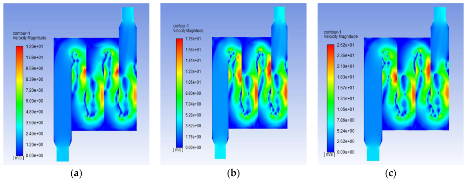
3.1. The Fluid Dynamics of the Flue Gas

To fully understand the motion state of the flue gas and further optimize the physical structure of the HE, a fluid simulation was conducted by regarding the flue gas as the thermal fluid, while the ambient air flowing into the HE was regarded as the cold fluid. The fluid model was set as the k-e model and the calculation steps were set to be 350. The velocity and the pressure distribution of the thermal fluid under different velocities (3, 5 and 7m·s⁻¹) of flue gas were investigated, and the detailed results are analyzed in Section 3.1.1 and 3.1.2.

3.1.1. The Velocity Distribution of the Flue Gas

The velocity nephograms for the $v_{fg}$ of 3, 5 and 7 m·s⁻¹ are depicted in Figure 4a–c, respectively. It can be concluded from the nephograms that the $v_{fg}$ is distributed evenly at the entrance of the HE, indicating that the $v_{fg}$ is stable at the HE entrance. However, the $v_{fg}$ close to the outside wall decreases rapidly and tends to be 0 at the first back bending, while the $v_{fg}$ close to the inner wall increases slowly; a similar phenomenon also occurs at the other three back bendings. The maximum $v_{fg}$ values were found in the middle of the two adjacent back bendings, and the maximum values for the different inlet flue gas velocities of 3, 5 and 7 m·s⁻¹ were 12.0, 17.7 and 25.27 m·s⁻¹, respectively. Interestingly, there is a vortex flow phenomenon after each back bending, which might be caused by the fact that the resistance between the flue gas flow and the inner surface of the FGD interferes with the flow of flue gas that further leads to the increase in the disorder of the flue gas flow, and finally forms the fluid vortex flow. Similar findings were reported by Guo, X. and Zhang, B. in a pipeline natural gas pressure-regulating process [38]. Moreover, it can also be found that the diameter of the vortex increases with the increase in $v_{fg}$, indicating that the flue gas temperature will be distributed more evenly if the $v_{fg}$ is increased, while correspondingly, the flow resistance will also be greater, just as was reported by Luo, X. in a “review of vortex tools toward liquid unloading for the oil and gas industry” [39].

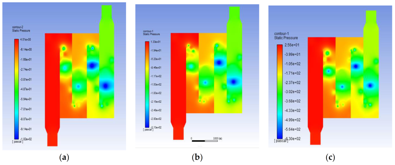
3.1.2. The Pressure Distribution of the Flue Gas

As analyzed above, the pressure drop in the thermal fluid is one of the most important indexes for matching the driving power of the induced draft fan, while the pressure distribution is the key factor affecting the pressure drop. Accordingly, the pressure distribution of the flue gas with different inlet velocities was investigated, and the results are shown in Figure 5.

Obviously, it can be concluded from the figures that the pressure at the entrance of the FGD is evenly distributed owing to the fact that the $v_{fg}$ in this area is stable; however, the pressure decreases rapidly after the back bending, just as in the trend of the $v_{fg}$ mentioned above, and a similar phenomenon arose in the other three back bendings. As a result, the pressure difference between the inlet and outlet of the HE is huge, and a greater driving force is needed. Similar to the analysis in Section 3.1, the inlet $v_{fg}$ is proportional to the outlet $v_{fg}$, and the outlet pressure is also proportional to the outlet $v_{fg}$, which might owe to the fact that the higher the inlet $v_{fg}$ is, the higher the inlet pressure will be even if the turbulence degree at the final stage increases with the decrease in $v_{fg}$. Moreover, the nephograms shown in Figure 5a–c indicate that there are six vortexes for each nephogram and that the low pressure areas are often located at the vortexes, while the pressure gradually decreases from the outside to the inside of the vortexes owing to the fact that the velocity at the center of the vortex is minimum. Moreover, there are two strong turbulence phenomena at the last two stages, which are the main areas hindering the flow of flue gas. From the perspective of the FGD design, the vortexes and the turbulence phenomenon should be avoided for the purpose of optimizing the allocation of the driving force. Accordingly, based on the analysis above, several recommendations can be made for optimizing the FGD, which are listed as follows:

(1)

A cambered surface design at the intersection of the vertical wall and transverse wall might be one of the effective methods to decrease the flow resistance of the flue gas.

(2)

A smooth and adiabatic wall material design may be one of effective methods to reduce flow resistance.

(3)

The drained cells on the wall in the last two chambers can be designed to help to avoid the vortex phenomenon and reduce flow resistance.

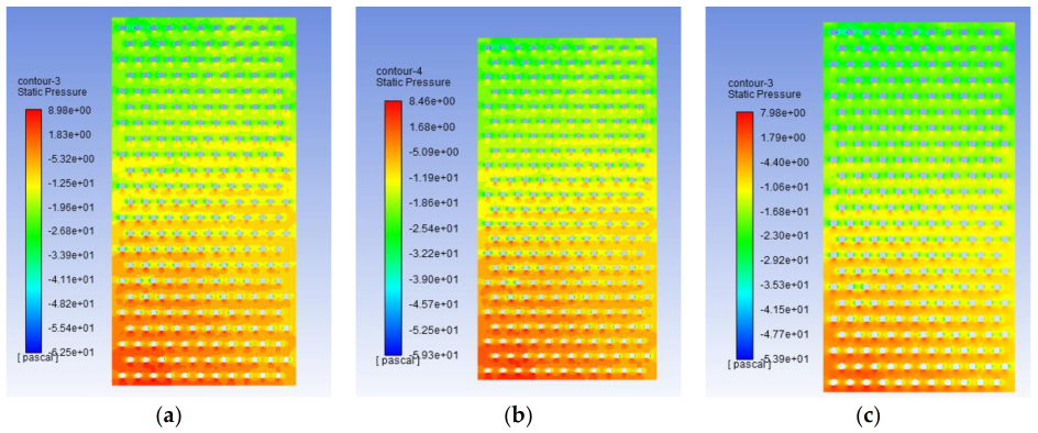
3.2. The Fluid Dynamics of the Cold Fluid

During the experimental period, the T₀ varied within a small range while the $R{H}_0$ varied within a relatively large range. Accordingly, the present work considers the $R{H}_0$ as the key factor affecting the heat exchange performance of the HE, and the velocity and the pressure distribution of the ambient air inlet into the HE were investigated under different relative humidities (80%, 85% and 90%) with a constant inlet $v_{air}$ of 3 m·s⁻¹. The detailed results are described in Section 3.2.1 and Section 3.2.2.

3.2.1. The Velocity Distribution of the Ambient Air into the HE

The velocity distributions corresponding to the different inlet ambient air $R{H}_0$ values of 80%, 85% and 90% are depicted in Figure 6a–c, respectively. As can be seen from the figures, the maximum $v_{air}$ for the $R{H}_0$ of 80%, 85% and 90% is 8.70, 8.66 and 8.57 m·s⁻¹, respectively, and the distributions of the $v_{air}$ in the three nephograms are also similar. Accordingly, it can be concluded that the $R{H}_0$ has a slight influence on the velocity distribution of the ambient air into the HE. In the initial stage of the ambient air flowing into the HE, the $v_{air}$ is distributed evenly, the flow path changes a little and the fluid flow is relatively smooth. However, with the increase in the flow path, the flow direction of the air demonstrates a slight bending trend, which might owe to the fact that the alternative arrangement of the pipe rows leads to the reduction in the fluid flow path, and then to the gradual expansion of the flow path. In other words, the fluid path flowing from the front row is significantly affected by the later one, and further leads to the change in the fluid flow path. Moreover, it can be also concluded from all the nephograms that in the middle of the HE, the $v_{air}$ decreases with the increase in the flow path owing to the fact that the resistance accumulation is also increased with the increase in the flow path. However, the $v_{air}$ close to the wall increases rapidly after half of the flow path is completed, which might be caused by the fact that cold fluid flows to both sides under interference from the tube bundle. The phenomenon might result in the insufficient heat exchange between the cold fluid and the tube bundle. The reduction in the distance between the tube bundle column and the wall of the HE might be an effective method to enhance the heat exchange performance of the HE, while a higher resistance will be needed instead. Therefore, it is necessary to figure out a suitable distance for enhancing the heat exchange performance while retaining the low flow resistance of the cold fluid.

3.2.2. The Pressure Distribution of the Ambient Air into the HE

The pressure distributions corresponding to the different inlet ambient air $R{H}_0$ values of 80%, 85% and 90% are depicted in Figure 7a–c, respectively. As can be seen from the figures, the inlet air pressure increases with the increase in $R{H}_0$, and the maximum pressure for the three nephograms is found to be at the entrance of the HE. At the beginning of the cold fluid flowing into the HE, the pressure distribution of the fluid tends to favor the left side of the HE, meaning the pressure is higher on the left side than on the right side. With the increase in the flow path, the pressure gradually decreases, especially for the fluid with an $R{H}_0$ of 90%, and the pressure begins to decrease gradually once about one-third of the flow path is completed, while for the fluid with an $R{H}_0$ of 80%, it begins to decrease gradually once about one-half of the flow path is completed. The pressure turning point of the fluid with 85% humidity is between the above-mentioned two transition points. During the outlet stage of the HE, the pressures of three different $R{H}_0$ values are basically the same, and thus, the pressure difference caused by the different inlet $R{H}_0$ fluids, in ascending order, are: 90%, 85% and 80%. Although a high pressure difference creates a high resistance cost, the high pressure difference is beneficial to the overall heat exchange performance of the HE. Accordingly, under the same inlet $R{H}_0$, although the higher humidity fluid brings a greater flow resistance and increases the complexity and flow resistance of the fluid, the heat exchange performance of the HE will be enhanced.

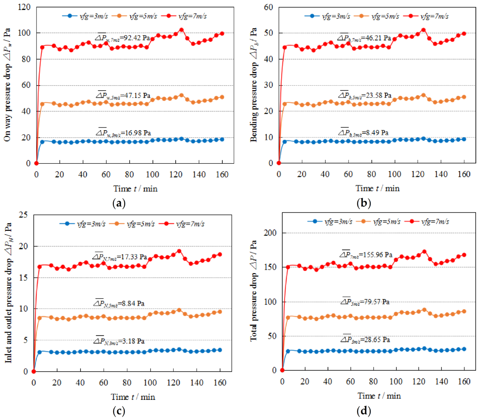
3.3. The Variations in Pressure Drop of the Flue Gas in the Air Duct over Time

In engineering applications, $\Delta p$ is one of the most important parameters to determine the power of the induced draft fan of the dryer, which consists of the $\Delta p_w$, $\Delta p_b$ and $\Delta p_n$. The variations in $\Delta p_w$, $\Delta p_b$, $\Delta p_n$ and $\Delta p$ under different inlet $v_{fg}$ values over $t$ are depicted in Figure 8a–d, respectively. As can be seen from Figure 8a, the $\Delta p_w$ increases with the increase in $v_{fg}$, and the $\Delta p_w$ for the $v_{fg}$ of 3, 5 and 7 m·s⁻¹ varies in the range of 15.92–18.79 Pa, 44.22–52.21 Pa and 86.67–102.33 Pa, respectively. It can be concluded that the stationarity of the $\Delta p_w$ decreases with the increase in $v_{fg}$, indicating that a low $v_{fg}$ may help to improve the stationarity of the heat exchange performance of the HE. Compared with the $\Delta p_w$, the corresponding value of $\Delta p_b$ is smaller than that of $\Delta p_w$ for the different $v_{fg}$ values, as is shown in Figure 8b. The average $\Delta p_b$ for the $v_{fg}$ of 3, 5 and 7 m·s⁻¹ is 16.98, 47.15 and 92.42 Pa, respectively. As can be seen from Figure 8c, the $\Delta p_n$ for the $v_{fg}$ of 3, 5 and 7m·s⁻¹ varies in the range of 2.98–3.52 Pa, 8.29–9.79 Pa and 16.25–19.19 Pa, respectively, and the $\Delta p_n$ decreases with the decrease in $v_{fg}$; the same trend is also shown in the $\Delta p$ analysis shown in Figure 8d. Similar findings have also been reported by Fei L et al. in their study of heat transfer and resistance characteristics of the H-type heat exchanger [40]. Moreover, it can be seen from the four figures that there was a fluctuation when t is 120 min, which may have been caused by the fact that the $v_{fg}$ was increased when the new fuel was added; the same fluctuation was reported in our previous work in a novel paddy grain dryer [41].

3.4. The Heat Exchange Performance between the Tube Bundle and the Cold Fluid

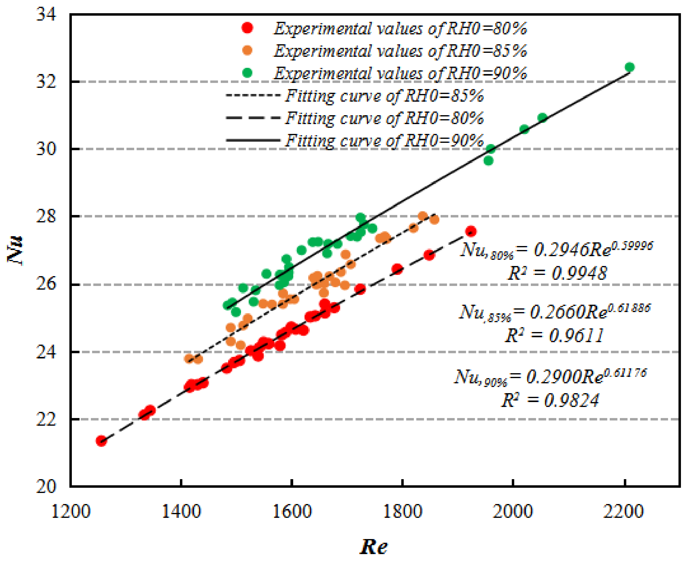
3.4.1. Influence of Relative Humidity of the Ambient Air on the Heat Exchange Performance

The physical meaning of the Nusselt number ($Nu$) is that it is not only a standard number to express the intensity of convective heat transfer, but also the ratio of heat conduction resistance and convective heat transfer resistance at the bottom layer of a fluid laminar flow [19]. Figure 9 depicts the relationship between the $Nu$ and $\mathrm{Re}$ for the different $R{H}_0$ values. As can be seen from the figure, the $Nu$ increases with the increase in the $\mathrm{Re}$ for all the $R{H}_0$ values; a similar finding was reported by Li et al. in regard to the heat transfer characteristic of a H-type finned elliptical tube [42]. Moreover, it can be found that the $\mathrm{Re}$ for the $R{H}_0$ of 80%, 85% and 90% is in the range of 1256.275–1923.969, 1414.882–1857.943 and 1484.459–2210.554, respectively, while the $Nu$ is in the range of 21.337–27.548, 23.759–28.001 and 25.156–32.415, respectively, which can be regarded as the reference parameters for designing and optimizing the HE. In order to quantitatively describe the relationship between the $Nu$ and $\mathrm{Re}$, three exponential models were established, and the corresponding equations are as follows:

$$N{\mathrm{u}}_{80\%}=0.2946{\mathrm{Re}}^{0.59996}, R^2=0.9946$$

(28)

$$N{\mathrm{u}}_{85\%}=0.2660{\mathrm{Re}}^{0.61886}, R^2=0.9611$$

(29)

$$N{\mathrm{u}}_{90\%}=0.2900{\mathrm{Re}}^{0.61176}$$

(30)

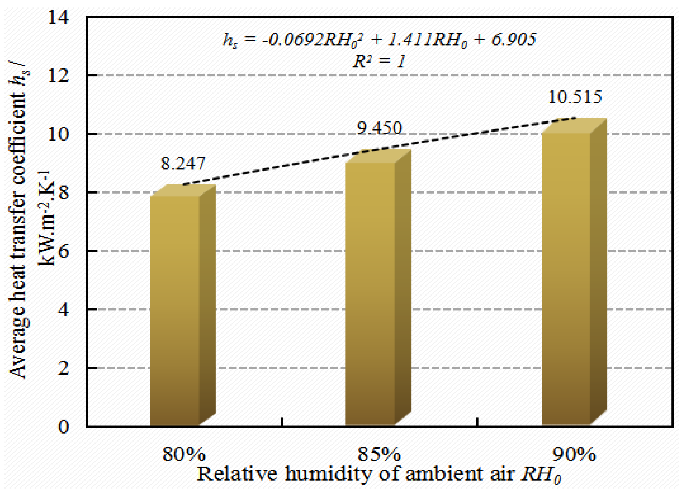
3.4.2. Influence of Relative Humidity of the Ambient Air on the Heat Transfer Coefficient

The $h_s$ is one of the most important parameters for the thermodynamic characteristics of heat exchangers, and is also the key index for studying the ventilation cooling mechanism, drying behavior and drying efficiency of agricultural product drying [42]. In the present work, the average $h_s$ under different $R{H}_0$ values (80%, 85% and 90%) were investigated, and the results are depicted in Figure 10. It can be concluded from Figure 10 that the h_s increases with the increase in $R{H}_0$, indicating that a high $R{H}_0$ can enhance the heat exchange performance between the HE and the inlet ambient air, which might be caused by the fact that the effective heat exchange surface of the HE tube bundle increases with the increase in $R{H}_0$. This finding was also reported by Yin et al. for the heat exchange performance in an air-source heat pump heater [43]. Moreover, the average $h_s$ under different $R{H}_0$ values of 80%, 85% and 90% was ascertained to be 8.247, 9.450 and 10.515 kW·m⁻²·K⁻¹; in other words, 8.247, 9.450 and 10.515 kJ of thermal energy are transferred when the ambient air temperature in a unit area increases by 1 K. In order to simplify the relationship between the $h_s$ and $R{H}_0$, a quadratic model was established where the R² is equal to 1, indicating that the model has a good fitting performance and can be used for monitoring the heat exchange performance of the HE.

3.4.3. Influence of Relative Humidity of the Ambient Air on the Tube Pressure Drop

In order to reasonably match the power of the IDF, the variations in the $\Delta p_t$ with different $R{H}_0$ values were investigated, and the results are shown in Figure 11. Similar to the variation trends in $h_s$, $\Delta p_t$ also increases with the increase in $R{H}_0$, which might be caused by the fact that the dynamic viscosity of the ambient air ($\mu$) increases with the increase in the $R{H}_0$ and leads to the decrease in the $\mathrm{Re}$, further leading to the increase in $\Delta p_t$, which can be summarized from Equations (11) and (16). A similar finding was reported by Shon, B. H et al. for the heat and pressure drop variation characteristics in a low GWP refrigerant in a brazed plate heat exchanger [44]. The average $\Delta p_t$ under different $R{H}_0$ values of 80%, 85% and 90% was ascertained to be 12.854, 14.623 and 16.138 Pa, respectively. A quadratic model describing the relationship between $\Delta p_t$ and $R{H}_0$ was established where the R² is equal to 1, indicating that the model has a good fitting performance and can be used as the reference for designing the distribution of the tube bundles.

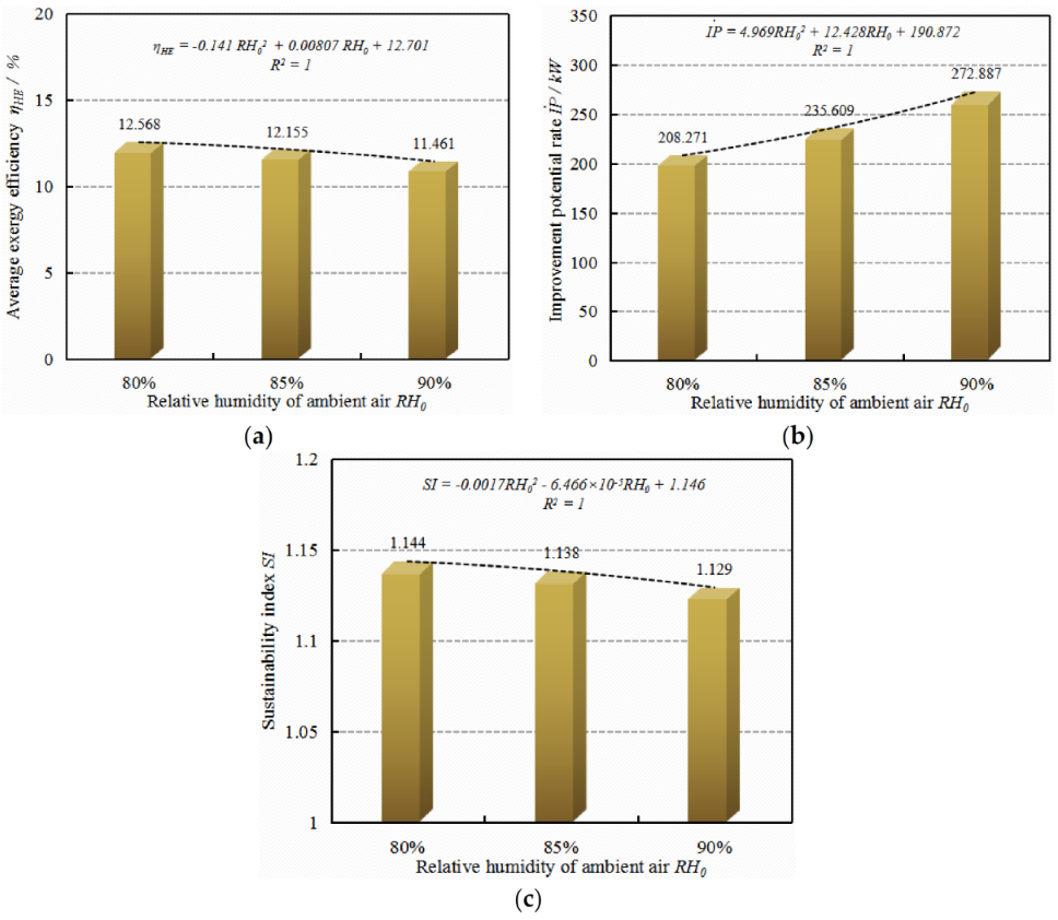
3.4.4. Influence of Relative Humidity of the Ambient Air on the Exergy Performance of the Heat Exchanger

Exergy analysis and its related concepts such as the sustainable index and improvement potential are widely used to evaluate the exergetic performance of an energy-intensive operation unit [45]. In the present work, the evaluation indexes including ${\eta }_{HE}$, $SI$ and $\stackrel{•}{IP}$ were used to investigate the exergetic performance of the HE. The variations in the ${\eta }_{HE}$, $\stackrel{•}{IP}$ and $SI$ with different $R{H}_0$ values are depicted in Figure 12a–c, respectively. Interestingly, it was found that the ${\eta }_{HE}$ decreases with the increase in the $R{H}_0$, which is contrary to the trend in $h_s$ shown in Section 3.4.2. The phenomenon might be caused by the fact that the humidity ratio of the air is proportionate to the relative humidity of the air, and the exergy of the air increases with the increase in the humidity ratio of the air, as is shown in Equations (18) and (23). Similar results were reported by Li C Y. et al. for the hot air drying process of grains [46]. Moreover, it can be seen from Figure 12a that the average ${\eta }_{HE}$ for the different $R{H}_0$ values of 80%, 85% and 90% is 12.57%, 12.16% and 11.46%, respectively. Though the ${\eta }_{HE}$ is slightly higher than that in some other industrial heat exchangers, such as the exergy efficiency (${\eta }_{HE}$ = 4.1%) of an air heat exchanger for the cooling of residential buildings [47], it should be further improved.

Improvement potential ($\stackrel{•}{IP}$) is an effective index for evaluating the improvement in the exergy efficiency for a process or a system. The variations in the $\stackrel{•}{IP}$ with different $R{H}_0$ values are depicted in Figure 12b. As can be seen from the figure, the $\stackrel{•}{IP}$ increases with the $R{H}_0$, and the average values for the $R{H}_0$ of 80%, 85% and 90% are found to be 208.27, 235.609 and 272.887 kW, respectively, indicating that they reach the goal of the maximum improvement in the exergy efficiency or minimized exergy loss (irreversibility). In 2001, Rosen and Dincer [48] proposed an interdisciplinary triangle covered by the exergy analysis. They proposed that the exergy is the confluence of energy, environment and sustainable development, and the exergy efficiency is directly proportionate to the sustainability. In this study, to investigate the sustainability of the HE under different ambient conditions, the variations in SI with different $R{H}_0$ values were investigated, and the results are shown in Figure 12c. It was found that the $SI$ decreases with the increase in $R{H}_0$, and the average values of $SI$ for the $R{H}_0$ of 80%, 85% and 90% are 1.144, 1.138 and 1.129, respectively, which are all lower than 2, indicating that the HE is in sustainable development [21]. Moreover, to establish the relationship between the $R{H}_0$ and the exergetic indexes (${\eta }_{HE}$, $SI$ and $\stackrel{•}{IP}$), three quadratic models with a good fitting performance (R² = 1) were developed. The equations are shown in the corresponding figures, and can be used for evaluating and predicting the exergetic performance of the HE.

4. Conclusions

The present work introduced a self-developed tube and shell heat exchanger for a corn drying system, and conducted the numerical simulation and experimental study on the fluid dynamics and exergetic performance of the heat exchanger. The detailed conclusions based on the main results are listed as follows:

(1)

The weak links of the heat transfer process for the heat exchanger are ascertained to be the last stages of the flue gas duct, the tube bundle back bendings, and the distance between the tube bundle column and the wall of the HE.

(2)

The $v_{fg}$ can significantly affect the heat transfer performance while the $R{H}_0$ slightly affects the heat transfer performance. Furthermore, it was found that a low $v_{fg}$ can help to improve the stationarity of the heat exchange performance of the HE.

(3)

The values of $\mathrm{Re}$ and $Nu$ varied in the range of 1256.275–2210.554 and 21.337–32.415, respectively. The average $h_s$ was ascertained to be above 8.274 kW·m⁻²·K⁻¹, while the $\Delta p$ was ascertained to be under 16.138 Pa.

(4)

The ${\eta }_{HE}$ and $SI$ decreased with the increase in the $R{H}_0$, while the increased with the increase in the $R{H}_0$. All the values of $SI$ were lower than 2, indicating that the heat exchanger is sustainable.

The main conclusions and the methodology can lay the fundamental basis for designing and optimizing the physical structure of the heat exchanger. Moreover, to fully understand the heat and exergy transfer characteristics of the heat exchanger, the influence of ambient air temperature on the fluid dynamics and the exergetic performance of the heat exchanger should be further investigated.

References

1. Mujumdar, A.S. Handbook of Industrial Drying, 3rd ed.; Taylor & Francis Group: Boca Raton, FL, USA; CRC Press: Boca Raton, FL, USA, 2006; pp. 134–156. [Google Scholar] [CrossRef]
2. Kudra, T. Energy aspects in drying. Dry Technol. 2004, 22, 917–932. [Google Scholar] [CrossRef]
3. Kemp, I.C. Fundamentals of Energy Analysis of Dryers, 2nd ed.; Wiley-VCH Verlag GmbH: Weinheim, Germany, 2011; pp. 5–46. [Google Scholar] [CrossRef]
4. Santivarangkna, C.; Kulozik, U.; Foerst, P. Effect of carbohydrates on the survival of lactobacillus helveticus during vacuum drying. Lett. Appl. Microbiol. 2010, 42, 261–276. [Google Scholar] [CrossRef] [PubMed]
5. Li, C.; Liao, J.J.; Yin, Y.; Mo, Q.; Chang, L.P.; Bao, W.R. Kinetic analysis on the microwave drying of different forms of water in lignite. Fuel Process. Technol. 2018, 176, 174–181. [Google Scholar] [CrossRef]
6. Sharma, G.P.; Verma, R.C.; Pathare, P.B. Thin-layer infrared drying of onion slices. J. Food Eng. 2005, 67, 361–366. [Google Scholar] [CrossRef]
7. Zbicinski, I. Equipment, technology, perspectives and modeling of pulse combustion drying. Chem. Eng. J. 2002, 86, 33–46. [Google Scholar] [CrossRef]
8. Omer, A.M. Performance, modeling, measurements and simulation of energy efficient for heat exchanger refrigeration and air conditioning. Adv. Robot. Autom. 2015, 5, 35–49. [Google Scholar] [CrossRef] [Green Version]
9. Sannervik, J.; Bolmstedt, U.; Traegardh, C. Heat transfer in tubular heat exchangers for particulate containing liquid foods. J. Food Eng. 1996, 29, 63–74. [Google Scholar] [CrossRef]
10. Xu, Z.; Jiang, X.; Liu, Z.; Hu, Y.; Li, Y. Experimental investigation of microbial fouling and heat mass transfer characteristics on ni-p modified surface of heat exchanger. J. Therm. Sci. 2020, 30, 271–278. [Google Scholar] [CrossRef]
11. Llopis, R.; Sanz-Kock, C.; Cabello, R.; Sánchez, D.; Torrella, E. Experimental evaluation of an internal heat exchanger in a CO2 subcritical refrigeration cycle with gas-cooler. Appl. Therm. Eng. 2015, 80, 31–41. [Google Scholar] [CrossRef] [Green Version]
12. Du, W.J.; Wang, P.L.; Cheng, L. Numerical simulation and experimental research on novel heat transfer surface. CIESC J. 2015, 66, 2070–2075. [Google Scholar] [CrossRef]
13. Wang, K.Y. Flow and Heat Transfer Analysis of a Novel Heat Exchanger with Rotated Aligned Tube Bank. Ph.D. Thesis, Shandong University, Jinan, China, 25 June 2018. [Google Scholar]
14. Akpinar, E.K.; Midilli, A.; Bicer, Y. The first and second law analyses of thermodynamic of pumpkin drying process. J. Food Eng. 2006, 72, 320–331. [Google Scholar] [CrossRef]
15. Chen, H.T.; Hsieh, Y.L.; Chen, P.C.; Lin, Y.F.; Liu, K.C. Numerical simulation of natural convection heat transfer for annular elliptical finned tube heat exchanger with experimental data. Int. J. Heat Mass Transf. 2018, 127, 541–554. [Google Scholar] [CrossRef]
16. Yu, X.F.; Wang, Z.Y.; Li, Q.Y.; Huang, W.H.; Lu, Y.A.; Yang, M. Numerical simulation of periodically fully developed flow and heat transfer in crossflow over intensive tube banks. J. Univ. Shanghai Sci. Technol. 2015, 37, 563–567. [Google Scholar] [CrossRef]
17. Shrikant, A.A.; Sivakumar, R.; Anantharaman, N.; Vivekenandan, M. CFD simulation study of shell and tube heat exchangers with different baffle segment configurations. Appl. Therm. Eng. 2016, 108, 999–1007. [Google Scholar] [CrossRef]
18. Córcoles-Tendero, J.I.; Belmonte, J.F.; Molina, A.E.; Almendros-Ibá?ez, J.A. Numerical simulation of the heat transfer process in a corrugated tube. Int. J. Therm. Sci. 2018, 126, 125–136. [Google Scholar] [CrossRef]
19. Vicente, P.G.; Garcia, A.; Viedma, A. Mixed convection heat transfer and isothermal pressure drop in corrugated tubes for laminar and transition flow. Int. Commun. Heat Mass Transf. 2004, 31, 651–662. [Google Scholar] [CrossRef]
20. Coskun, C.; Oktay, Z.; Ilten, N. A new approach for simplifying the calculation of flue gas specific heat and specific exergy value depending on fuel composition. Energy 2009, 34, 1898–1902. [Google Scholar] [CrossRef]
21. Beigi, M.; Tohidi, M.; Torki-Harchegani, M. Exergetic Analysis of Deep-Bed Drying of Rough Rice in a Convective Dryer. Energy 2017, 140, 374–382. [Google Scholar] [CrossRef]
22. Davidzon, M.I. Newton’s law of cooling and its interpretation. Int. J. Heat Mass Transf. 2012, 55, 5397–5402. [Google Scholar] [CrossRef]
23. Feng, J.S.; Dong, H.; Gao, J.Y.; Liu, J.Y.; Liang, K. Exergy transfer characteristics of gas-solid heat transfer through sinter bed layer in vertical tank. Energy 2016, 111, 154–164. [Google Scholar] [CrossRef]
24. Shuyan, W.; Guodong, L.; Yanbo, W.; Juhui, C.; Yongjian, L.; Lixin, W. Numerical investigation of gas-to-particle cluster convective heat transfer in circulating fluidized beds. Int. J. Heat Mass Transf. 2010, 53, 3102–3110. [Google Scholar] [CrossRef]
25. Paulo, E.B.D.M.; Villanueva, H.H.S.; Sérgio, S.; Donato, G.H.B.; Ortega, F.D.S. Heat transfer, pressure drop and structural analysis of a finned plate ceramic heat exchanger. Energy 2017, 120, 597–607. [Google Scholar] [CrossRef]
26. Yu, J.Z. Principle and Design of Heat Exchanger. Ph.D. Thesis, Beihang University, Beijing, China, 18 June 2006. [Google Scholar]
27. Khanali, M.; Aghbashlo, M.; Rafiee, S.; Jafari, A. Exergetic performance assessment of plug flow fluidised bed drying process of rough rice. Int. J. Exergy 2013, 13, 387–408. [Google Scholar] [CrossRef]
28. Yildirim, N.; Genc, S. Energy and exergy analysis of a milk powder production system. Energy Convers. Manag. 2017, 149, 698–705. [Google Scholar] [CrossRef]
29. Aghbashlo, M.; Mobli, H.; Rafiee, S. Energy and exergy analyses of the spray drying process of fish oil microencapsulation. Biosyst. Eng. 2012, 111, 229–241. [Google Scholar] [CrossRef]
30. Sarker, M.S.H.; Ibrahim, M.N.; Abdul, A.N. Energy and exergy analysis of industrial fluidized bed drying of paddy. Energy 2015, 84, 131–138. [Google Scholar] [CrossRef]
31. Tohidi, M.; Sadeghi, M.; Torki-Harchegani, M. Energy and quality aspects for fixed deep bed drying of paddy. Renew. Sustain. Energy Rev. 2017, 70, 519–528. [Google Scholar] [CrossRef]
32. Soufiyan, M.M.; Dadak, A.; Hosseini, S.S.; Nasiri, F.; Dowlati, M.; Tahmasebi, M. Comprehensive exergy analysis of a commercial tomato paste plant with a double-effect evaporator. Energy 2016, 111, 910–922. [Google Scholar] [CrossRef]
33. Van, G.W. Energy policy: Fairly tales and factualities. In Innovation and Technology-Strategies and Policies; Soares, O.D.D., da Martins Cruz, A., Costa Pereira, G., Soares, I.M.R.T., Reis, A.J.P.S., Eds.; Kluwer Academic Publisher: Dordrecht, The Netherlands, 1997; pp. 93–105. [Google Scholar]
34. Rosen, M.A.; Dincer, I.; Kanoglub, M. Role of exergy in increasing efficiency and sustainability and reducing environmental impact. Energy Policy 2008, 36, 128–137. [Google Scholar] [CrossRef]
35. Holman, J.P. Experimental Methods for Engineers, 7th ed.; McGraw-Hill: New York, NY, USA, 2001; pp. 48–143. [Google Scholar]
36. Coleman, H.W.; Steele, W.G. Experimentations and Uncertainty Analysis for Engineers, 2nd ed.; Wiley-Interscience: New York, NY, USA, 1999. [Google Scholar]
37. Ullum, T.; Sloth, J.; Brask, A.; Wahlberg, M. Predicting Spray Dryer Deposits by CFD and an Empirical Drying Model. Dry. Technol. 2010, 28, 723–729. [Google Scholar] [CrossRef]
38. Guo, X.; Zhang, B. Experimental investigation on a novel pressure-driven heating system with ranque–hilsch vortex tube and ejector for pipeline natural gas pressure regulating process. Appl. Therm. Eng. 2019, 152, 634–642. [Google Scholar] [CrossRef]
39. Luo, X.; Yang, L.; Yin, H.; He, L.; Lü, Y. A review of vortex tools toward liquid unloading for the oil and gas industry. Chem. Eng. Process. 2019, 145, 107679. [Google Scholar] [CrossRef]
40. Li, F.; Shi, Y.; Sun, F.; Li, Z. Experimental research on heat transfer and resistance characteristics of h-type finned elliptical tubes. Proc. CSEE 2014, 34, 2261–2266. [Google Scholar] [CrossRef]
41. Li, B.; Li, C.; Li, T.; Zeng, Z.; Ou, W.; Li, C. Exergetic, energetic, and quality performance evaluation of paddy drying in a novel industrial multi-field synergistic dryer. Energies 2019, 12, 4588. [Google Scholar] [CrossRef] [Green Version]
42. Cong, D.T.; Haddad, M.A.; Rezzoug, Z.; Laurent, L.; Karim, A. Dehydration by successive pressure drops for drying paddy rice treated by instant controlled pressure drop. Dry. Technol. 2008, 26, 443–451. [Google Scholar] [CrossRef]
43. Yin, S.Y.; Wu, Z.J.; Li, D.M. The Effect of Air Relative Humidity on Performance of Air-source Heat Pump Water Heater. J. Shunde Polytech. 2011, 11, 1–3. [Google Scholar] [CrossRef]
44. Shon, B.H.; Jung, C.W.; Kwon, O.J.; Choi, C.K.; Kang, Y.T. Characteristics on condensation heat transfer and pressure drop for a low gwp refrigerant in brazed plate heat exchanger. Int. J. Heat Mass Transf. 2018, 122, 1272–1282. [Google Scholar] [CrossRef]
45. Li, B.; Li, C.; Huang, J.; Li, C. Exergoeconomic analysis of corn drying in a novel industrial drying system. Entropy 2020, 22, 689. [Google Scholar] [CrossRef]
46. Li, C.Y.; Mai, Z.W.; Fang, Z.D. Analytical study of grain moisture binding energy and hot air drying dynamics. Trans. Chin. Soc. Agric. Eng. 2014, 30, 236–242. [Google Scholar] [CrossRef]
47. Dastmalchi, M.; Boyaghchi, F.A. Exergy and economic analyses of nanoparticle-enriched phase change material in an air heat exchanger for cooling of residential buildings. J. Energy Storage 2020, 32, 101705. [Google Scholar] [CrossRef]
48. Rosen, M.A.; Dincer, I. Exergy as the confluence of energy, environment and sustainable development. Int. J. Exergy 2001, 1, 3–13. [Google Scholar] [CrossRef]
Figure 1. The scene graph of the drying system.
Applsci 13 02966 g001
Figure 2. The scene graphs of the HE and the 3D model of the HE: (a) scene graph of HE; (b) 3D model of HE.
Applsci 13 02966 g002
Figure 3. The two dimensional grids of the cold fluid (a) and thermal fluid (b).
Applsci 13 02966 g003
Figure 4. The velocity distributions corresponding to the different inlet flue gas velocities. (a) Velocity nephogram for v f g = 3 m·s−1. (b) Velocity nephogram for v f g = 5 m·s−1. (c) Velocity nephogram for v f g = 7 m·s−1.
Applsci 13 02966 g004
Figure 5. The pressure distributions corresponding to different inlet flue gas velocities. (a). Pressure nephogram for v f g = 3 m·s−1. (b). Pressure nephogram for v f g = 5 m·s−1. (c). Pressure nephogram for v f g = 7 m·s−1.
Applsci 13 02966 g005
Figure 6. The velocity distributions corresponding to different relative humidities of inlet ambient air. (a) Velocity nephogram for R H 0 = 80 % . (b) Velocity nephogram for R H 0 = 85 % . (c) Velocity nephogram for R H 0 = 90 % .
Applsci 13 02966 g006
Figure 7. The pressure distributions corresponding to different relative humidities of inlet ambient air. (a) Pressure nephogram for R H 0 = 80 % . (b) Pressure nephogram for R H 0 = 85 % . (c) Pressure nephogram for R H 0 = 90 % .
Applsci 13 02966 g007
Figure 8. The variations of Δ p w (a), Δ p b (b), Δ p n (c) and Δ p (d) under different inlet v f g values over t .
Applsci 13 02966 g008
Figure 9. The relationship between the N u and Re for different R H 0 values.
Applsci 13 02966 g009
Figure 10. The variations in average h s with different R H 0 values.
Applsci 13 02966 g010
Figure 11. The variations in Δ p t with different R H 0 values.
Applsci 13 02966 g011
Figure 12. The variations in η H E (a), I P (b) and S I (c) with R H 0 values.
Applsci 13 02966 g012