Inter-Seasonal Estimation of Grass Water Content Indicators Using Multisource Remotely Sensed Data Metrics and the Cloud-Computing Google Earth Engine Platform

Abstract

Indicators of grass water content (GWC) have a significant impact on eco-hydrological processes such as evapotranspiration and rainfall interception. Several site-specific factors such as seasonal precipitation, temperature, and topographic variations cause soil and ground moisture content variations, which have significant impacts on GWC. Estimating GWC using multisource data may provide robust and accurate predictions, making it a useful tool for plant water quantification and management at various landscape scales. In this study, Sentinel-2 MSI bands, spectral derivatives combined with topographic and climatic variables, were used to estimate leaf area index (LAI), canopy storage capacity (CSC), canopy water content (CWC) and equivalent water thickness (EWT) as indicators of GWC within the communal grasslands in Vulindlela across wet and dry seasons based on single-year data. The results illustrate that the use of combined spectral and topo-climatic variables, coupled with random forest (RF) in the Google Earth Engine (GEE), improved the prediction accuracies of GWC variables across wet and dry seasons. LAI was optimally estimated in the wet season with an RMSE of 0.03 m⁻² and R² of 0.83, comparable to the dry season results, which exhibited an RMSE of 0.04 m⁻² and R² of 0.90. Similarly, CSC was estimated with high accuracy in the wet season (RMSE = 0.01 mm and R² = 0.86) when compared to the RMSE of 0.03 mm and R² of 0.93 obtained in the dry season. Meanwhile, for CWC, the wet season results show an RMSE of 19.42 g/m⁻² and R² of 0.76, which were lower than the accuracy of RMSE = 1.35 g/m⁻² and R² = 0.87 obtained in the dry season. Finally, EWT was best estimated in the dry season, yielding a model accuracy of RMSE = 2.01 g/m⁻² and R² = 0.91 as compared to the wet season (RMSE = 10.75 g/m⁻² and R² = 0.65). CSC was best optimally predicted amongst all GWC variables in both seasons. The optimal variables for estimating these GWC variables included the red-edge, near-infrared region (NIR) and short-wave infrared region (SWIR) bands and spectral derivatives, as well as environmental variables such as rainfall and temperature across both seasons. The use of multisource data improved the prediction accuracies for GWC indicators across both seasons. Such information is crucial for rangeland managers in understanding GWC variations across different seasons as well as different ecological gradients.

1. Introduction

Plant water content (PWC) is one of the most critical parameters of land surface–atmosphere interactions, considerably affecting the seasonal terrestrial water cycle [1]. This is because the quantity of water contained in the vegetation canopy structure has profound effects on physiological processes such as evapotranspiration, and photosynthesis, which directly affect an ecosystem’s water balance [2,3]. Thus, vegetation-water-related properties are critical for understanding key components of the hydrological cycle to derive insights into catchment water variation.

Several interrelated physiological indicators have been used to assess vegetation water conditions at different structural levels. The commonly used indicators include relative water content [4], leaf water potential [5], equivalent water thickness [6], live fuel moisture content [7], canopy water content [8], canopy storage capacity, and stomatal conductance [9]. Amongst these, canopy storage capacity (CSC) is the volume of water that can be retained in plant canopies [10]. The CSC directly influences hydrology through rainfall interception and altering infiltration, thus affecting water redistribution [11]. Canopy water content (CWC) is the total water content per unit area of a ground surface, which depends on the balance between water losses from transpiration and water uptake from the soil [8]. Equivalent water thickness (EWT) is the quantity of water content per unit leaf area. It plays a critical role in eco-hydrological processes such as evaporation and transpiration [12]. The reflectance of vegetation water content is affected by many biophysical parameters, and it is challenging to separate the contribution of the leaf area index (LAI) and water content from remotely sensed data at the leaf level [13]. In this regard, the LAI and the above-explained water content indicators are of interest in this study.

In the past few decades, water content indicators have been utilized as a proxy for crop water stress or drought assessment and monitoring [14,15,16], prediction of ecosystems’ susceptibility to wildfire [17,18] and in forestry studies [11,19]. However, more effort needs to be made to study the seasonal variability in vegetation water content indicators specifically in the context of grassland ecosystems. By virtue of their location, being mostly in catchment areas, the grass water content (GWC) of these ecosystems significantly impacts on various hydrological processes since vegetation water content can be assumed to reflect the hydrological conditions of the antecedent hydrological year [20]. GWC relates to the quantity of water contained in grass. Since GWC indicators are closely related to hydrological variables, their estimation can be helpful for the hydrological modelling of surface run-off, recharge, and groundwater processes and soil moisture budget.

Remote sensing has been widely recognized to be invaluable in providing effective, non-invasive and reliable techniques for assessing water content indicators [21]. Remote sensing sensors, including multispectral [22,23,24] and hyperspectral [10,25,26] sensors, have been applied for vegetation water content monitoring. For instance, MODIS and Landsat satellites provide Earth observation data free of charge, which may be used for global environmental monitoring [27,28]. However, the multispectral sensors onboard these satellites are associated with a low spectral resolution, thus posing a challenge to optimally exploit the comprehensive water absorption features in the short-wave infrared region (SWIR) [29]. Although hyperspectral sensors are renowned for their high accuracy in monitoring vegetation water conditions, they are coupled with high prices, yet they cover a small spatial extent [30].

Recent advancement in Earth observation sensors has seen the advent of free-of-charge data from Sentinel-2, which is equipped with a multispectral imager (MSI), providing an opportunity for robust estimation of vegetation-water-related properties [11]. The Sentinel-2 MSI offers the best combination of high spatial (i.e., up to 10 m pixel resolution), spectral (i.e., 13 bands), and optimal temporal sampling resolution of 5 days, making it suitable for characterizing the spatiotemporal variations in vegetation attributes [31]. Moreover, Sentinel-2 MSI incorporates critical red-edge (RE) bands, which are centred at 705, 740, and 783 nm of the electromagnetic spectrum [11]. Specifically, the RE is the section of the spectrum where there is rapid change in vegetation spectral reflectance; hence, it can be used to monitor the functioning of vegetation [16,32].

Meanwhile, the literature underscores the performance of spectral derivatives such as vegetation indices in estimating vegetation attributes such as water content, amongst others [15,33]. The most widely used vegetation indices in the literature are derived from the visible and near-infrared region (NIR) wavelengths [15,33]. Meanwhile, the SWIR, which is heavily influenced by water in plant tissues, also plays a significant role in mapping and monitoring moisture content [34]. Thus, the use of moisture-sensitive indices derived from longer wavelengths such as NIR and SWIR reflectance could be more viable for monitoring vegetation water content [35]. Other than optical spatial data, site-specific spatial data such as topographic and climate-related data are critical and required to improve the accuracy of optical models.

Topographic variables derived from digital elevation models such as the Shuttle Radar Topographic Mission (SRTM) can effectively increase the accuracy of vegetation monitoring [36,37]. Specifically, variations in topographic metrics such as the slope, topographic position index, state of curvature, and aspect are directly linked to vegetation aspects, such as sunlight and temperature, while indirectly linked to other aspects, such as soil moisture and soil quality [38,39]. Furthermore, climatic variables such as rainfall and temperature are critical factors controlling photosynthetic activities in vegetation as well as foliar water content variation [40]. Specifically, seasonal precipitation and temperature result in soil moisture content variations, which affect vegetation water content despite the impact of topographic variations [41]. However, the interacting influence of seasonal precipitation and temperature with topographic variations on GWC indicators has not been extensively researched, especially in communal grazing lands. Since topographic and climatic factors have been proven to be important variables in facilitating the spatial distribution of vegetation water content, there is a need to assess and understand the interacting influence of seasonality and topo-climatic variables on the spatial variability of grassland water content indicators.

Cloud-processing systems, such as the Google Earth Engine (GEE), provide a safe, efficient, and advanced platform designed to effectively deal with the challenges of storing, computing, processing, and analysing huge datasets [42,43]. The GEE provides free access to global time-series satellite and other ancillary data collected over 40 years, thus allowing a vast amount of computation analyses to be produced for unprecedented time and extent scales [44,45]. Importantly, the GEE platform provides users with a convenient environment for interactive data and algorithm development via its internet-based Python Application Programming Interfaces (APIs) and JavaScript web-based Interactive Development Environment (IDE) [42,46]. The high-performance computing capacity of the GEE for environmental monitoring has been demonstrated in several applications, such as soil erosion assessment [47,48], burned area mapping [49,50], hydrology [51,52], agriculture [53,54], and landcover mapping [55,56], as well as in vegetation mapping and monitoring [57,58].

Sibanda, Mutanga [12] reported that grass-water-related parameters can be optimally estimated using the combined use of spectral data and environmental variables. Unfortunately, the work by Sibanda, Mutanga [12] was a snapshot-type of analysis where only one image and one season were considered. This study sought to test the utility of multisource data in estimating the LAI, CSC, CWC, and EWT within communal grasslands across wet and dry seasons. It was hypothesized that integrating multisource data with a robust machine learning algorithm would improve the prediction accuracies of GWC indicators as a step towards building spatially explicit communal rangeland monitoring frameworks.

2. Materials and Methods

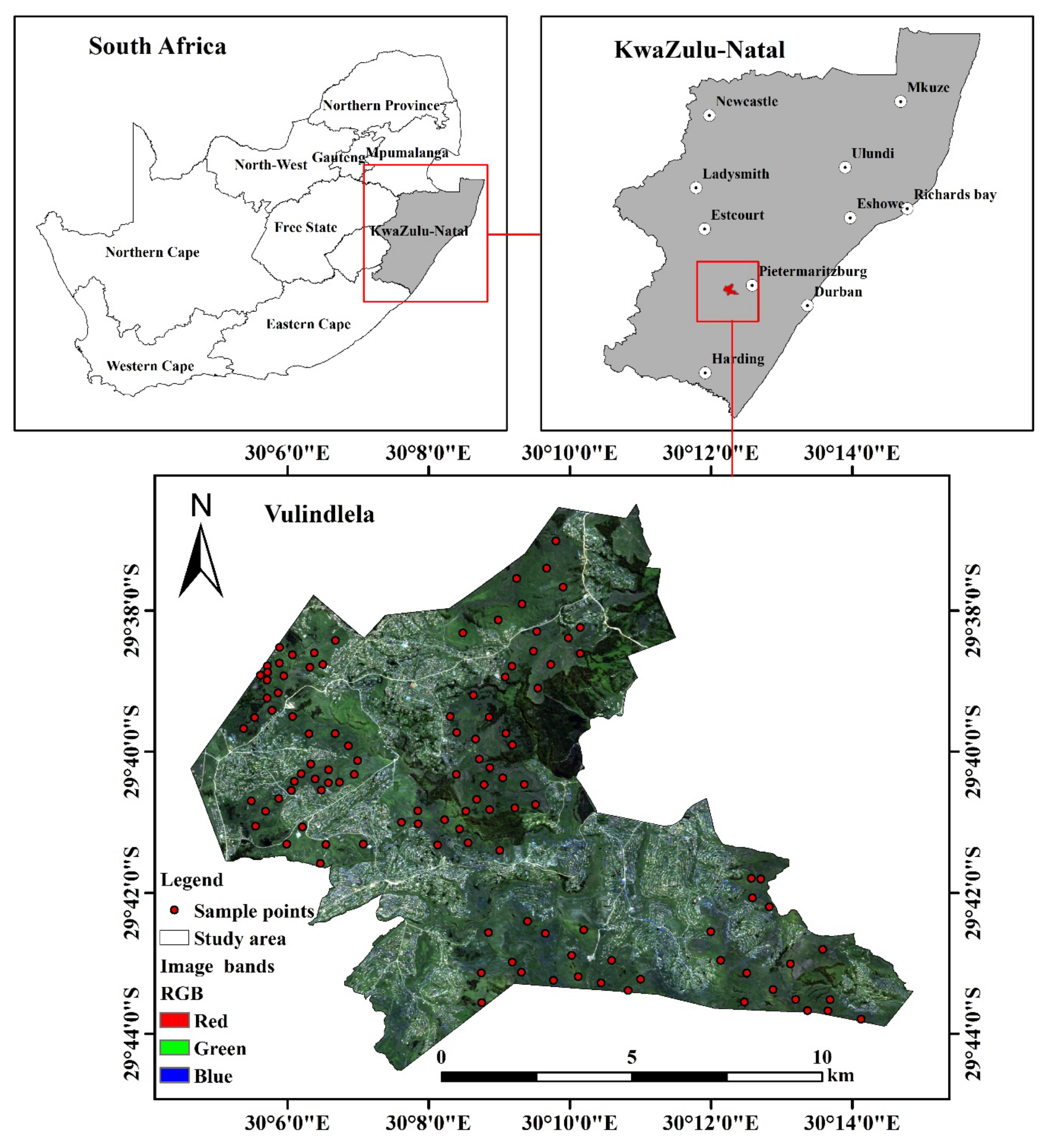
2.1. Study Area Description

This study was conducted in Vulindlela, a communal area located in Kwa-Zulu Natal Province, on the east coast of South Africa (Figure 1). The study area is predominantly rugged, with mountainous at an altitude range of 1273–1412 above sea level [59,60,61]. The soils are generally loam in the valley sides, and coarse-grained in the upper slopes due to rocky surfaces [61]. The mean annual rainfall of the area is 979 mm. The maximum monthly rainfall occurs in January [62]. The annual minimum and maximum mean temperatures are 10.3 °C and 21.9 °C, respectively [12]. The driest month with the lowest temperatures is July. The study area is located in a subtropical climate, characterized by a standard Southern Africa bimodal climate. The wet season occurs from September to March and the dry season from April to August [63,64]. The study area is mainly a mesic subtropical grassland biome. Mesic grasslands in South Africa are characterized by Sorghum bicolour, Aristida junciformis, Eragrostis tenuifolia, Alloteropsis semialata, Tristachya leucothrix, Themeda triandra, Paspalum urvillei, Panicum maximum, and Setaria sphacelate, amongst other grass species [65]. However, the dominant grass species in Vulindlela is Aristida junciformis. The optimal growing period of these species occurs from October to April [66]. Vulindlela is a good example of a predominantly rural community in which land is managed using the communal ownership approach [67]. The primary source of livelihood in Vulindlela is livestock farming, and communities depend on grasslands as grazing grounds for their livestock. This highlights the need to provide an efficient and cost-effective strategy for managing this natural resource.

2.2. Field Sampling Strategy and Water Content Indicator Measurements

Field data for the wet season were collected between 27 and 31 March 2022. This was meant to capture the peak water content period after the grass had responded to the maximum rainfall occurring in January. The dry season data were collected between 16 and 20 June when the GWC was low due to senescence. Although the driest month with the lowest temperatures is July, the communities in Vulindlela initiate seasonal burning of grass in June to stimulate new growth for livestock, making it impossible for data collection to be conducted in July.

One hundred and thirteen 10 m × 10 m quadrats were established 150 m apart using a purposive sampling strategy. A plot size of 10 m by 10 m was chosen in this study to ensure that all sampled areas were within the confines of Sentinel-2 MSI bands. Consequently, the 150 m distance was chosen to account for possible ground truth satellite image geolocation errors. Within each plot, two 1 m × 1 m sub-quadrats were randomly established within the 10 m plots for clipping grass. A handheld Trimble Global Positioning System (GPS) with a sub-meter accuracy was used to collect the centre co-ordinates of the sub-quadrats. The co-ordinate points were stored as waypoints and later used for navigation in the dry season data collection. Grass was clipped within each sub-quadrat, placed in brown paper bags, and correctly labelled. The fresh weight (FW) of sampled biomass was instantly weighed using a calibrated scale with a 0.5 g measurement error. The samples were taken to the laboratory and placed in the oven at 105 °C. For dry weight (DW), the samples were weighed consistently until a constant dry weight was reached (48–72 h).

LAI was also measured within each sub-plot using a portable handheld ground-based and non-destructive LAI 2200 plant canopy analyser (LI-COR Biosciences, Lincoln, NE, USA). Specifically, in measuring LAI, five readings were conducted: one above the grass canopy and four below the grass canopy. Field measurements for LAI were conducted between 12:00 noon and 14:00 as this is the optimal period of the day for vegetation photosynthetic activity [68].

2.3. Measurement of Grass Water Content Elements

The LAI (A), FW, and DW were used as input variables to compute GWC indicators. CSC was computed using the von Hoyningen-Huene (1981) model as follows:

S^c_max (mm) = 0.935 + 0.498 (LAI) − 0.00575 (LAI²),

(1)

where S^c_max is the CSC.

The von Hoyningen-Huene (1981) model is an accurate, non-species-specific model for the estimation of the maximum CSC [69]. The model was chosen for this study following its successful application within South Africa [10,11,12].

CWC was calculated based on the following equation:

CWC (g/m⁻²) = FW − DW.

(2)

EWT was calculated as follows:

$$\mathrm{EWT} (\mathrm{g}/{\mathrm{m}}^{-2})=\frac{\left(\mathrm{FW}-\mathrm{DW}\right)}{\mathrm{A}}$$

(3)

After retrieving all the GWC variables, they were averaged and integrated with the GPS points on an Excel spreadsheet. The data were then converted into separate point map shapefiles using ArcGIS 10.6 software. The shapefiles were then uploaded on the GEE platform so they could be overlaid with spectral data for further analysis.

2.4. Sentinel-2 MSI Data Acquisition

Sentinel 2 MSI Level 2A remotely sensed data were imported from Copernicus in the GEE data catalogue. Sentinel 2 is a pair of twin satellites (Sentinel-2A and Sentinel-2B) in the same orbit, phased 180° apart, operating at an altitude of 786 km, and designed to provide medium-spatial-resolution imagery in global environmental monitoring [70]. Both satellites are equipped with an MSI deriving data from 13 spectral channels along a 290 km sun-synchronous orbital path [71]. The two-satellite constellation provides a temporal resolution of 5 days under cloud-free conditions [72], which makes it suitable for detecting seasonal changes in grass productivity. Specifically, the GEE provides Level 2A products derived from Sentinel-2A that are readily processed by the Sentinel-2 atmospheric correction processor (Sen2Cor) as a default configuration to provide orthorectified atmospherically corrected surface reflectance [73].

Remotely sensed imagery with dates that coincided with the field data collection dates for both seasons were acquired. The filter image collection by date function was used to acquire images in the date range that coincided with the time when field surveys were conducted. This is necessary since changes in atmospheric conditions between on-site data collection and satellite data acquisition may affect grass properties and might alter model accuracy [74]. Prior to image downloading, the cloud pixel percentage was set to 10% to filter out Sentinel-2 scenes with a cloud cover of more than 10%. Subsequently, the median reducer function was applied to create a single image by calculating the median of all values at each pixel across the stack of all matching bands. The study area shapefile was imported, and the image was filtered to narrow it to the location of the region of interest. The ground sampling distance (GSD) of the Sentinel-2 MSI is divided into spectral bands with 4 bands (10 m), 6 bands (20 m), and 3 bands (60 m). Bands acquired at 60 m GSD (1, 9, and 10) were not included in this study because they are designed for detecting atmospheric characteristics and are unsuitable for vegetation analysis [75]. As a result, only 10 bands were selected from the image collection and utilized in this study. The Sentinel-2 MSI bands were resampled to a spectral resolution of 10 m to give all the bands the same pixel size.

2.5. Selection of Spectral Indices

The prediction of water content in vegetation using spectral indices mostly depends on the reflectance behaviour of water molecules in the leaves to various sections of the electromagnetic spectrum [76]. For instance, high foliar water content in vegetation is highly sensitive to water absorption features in the SWIR section, which explains the reflectance of vegetation in these regions [77]. Additionally, the RE region is sensitive to vegetation chlorophyll absorption, which is directly related to water content [78,79]. In comparison to other indices, water-sensitive as well as RE-based vegetation indices may have an advantage of accurate estimation of grass-leaf-water-related elements. In this regard, this study specifically evaluates the potential of water-sensitive spectral vegetation indices (which provide the absolute measure of plant water content) as well as the RE-region-based spectral vegetation indices in estimating GWC. The vegetation index formulas were identified and selected from the literature, whereas the other formulas were derived from the Index Database available online (https://www.indexdatabase.de/, accessed on 10 August 2022) and computed in the GEE platform (

Table 1. Spectral vegetation indices used in this study.

VI	VI Formula	Sentinel-2 Bands	References
Normalized Difference Water Index (NDWI)	$\frac{NIR-SWIR}{NIR+SWIR}$	B8, B12	[80]
Modified Normalized Difference Water Index (MNDWI)	$\frac{Green-SWIR}{Green+SWIR}$	B3, B11	[81]
Normalized Difference Infrared Index (NDII)	$\frac{NIR-SWIR}{NIR+SWIR}$	B8, B11	[82]
Moisture Stress Index (MSI)	$\frac{SWIR}{NIR}$	B11, B8	[83]
Normalized Difference Red Edge (NDRE)	$\frac{NIR-RE}{NIR+RE}$	B8, B5	[84]
Red-edge Ratio Index 1 (RRI1)	$\frac{ NIR}{RE}$	B8, B5	[85]
Red-edge 1 (Rededge1)	$\frac{RE}{RED}$	B5, B4	[86]
Red-edge 2 (Rededge2)	$\frac{RE-RED}{RE+RED}$	B5, B4	[86]
Red-edge Normalized Difference Vegetation index (NDVI705)	$\frac{ RE2-RE1}{RE2+RE1}$	B6, B5	[87]

).

2.6. Topo-Climatic Variables

Topographic variables are classified into three main groups: local (elevation, slope, land surface curvature), which examines surface geometry specific to a point on the land surface; nonlocal (flow accumulation, catchment area, relief), which is influenced by the relative location of a specific point on the land surface; and combined topographic metrics (topographic wetness index), which integrate both the local and nonlocal topographic metrics [88,89,90,91,92]. For extracting topographic indices, a 30 m × 30 m SRTM DEM was downloaded from the GEE. Twenty-three topographic variables (

Table 2. Topographic variables used in this study as explained in Odebiri, Mutanga [39].

Topographic Variable	Description
Slope	Degree of inclination of land surface
Elevation	Height above sea level
Aspect	Compass direction of a slope
Minimum curvature	Lowest deviation from slope curve
Maximum curvature	Highest deviation from slope curve
Longitudinal curvature	Explains the flowing speed of a substance downslope
Cross-section curvature	Explains the divergence or convergence of a flowing substance
Profile curvature	Represents morphology of the topography
General curvature	Total curvature of the surface
Plan curvature	Horizontal curvature of contour lines
Catchment area	Run-off water flow, forming a waterway
Positive openness	Dominance of a landscape location
Negative openness	Enclosure of a landscape location
Standardized height	Slope position and height
Normalized height	Slope position and height
Valley depth	Relative height of a valley
Convergence index	Calculates valleys and ridges
Wind effect	Effects of the direction and speed of wind on the surface
Direct insolation	Incoming solar radiation
Terrain roughness index	Surface heterogeneity
Topographic wetness index	Quantifies topographic control on hydrological processes
Skyview factor	Visible sky
Mass balance index	Terrain morphometry

) were derived using SAGA QGIS (2.3.2) and ArcGIS 10.6 software. Rainfall and temperature datasets were acquired from South African Weather Services (SAWS). The climatic datasets were averaged per season and resampled to a 10 m spatial resolution to give them the same pixel size as the remotely sensed imagery. The topo-climatic variables were then imported into the GEE as shapefiles for further analysis.

2.7. Spatial Analysis

All statistical analysis in this study was performed using the GEE platform. A random forest (RF) ensemble was used to predict grass water content elements. RF is an ensemble learning technique that was first proposed by Breiman [93]. It is considered a robust regression technique that uses multiple decision trees to make predictions [94]. In RF, a large number of decision trees are randomly created (with replacement) from the original training data and variables [95]. Each node per regression tree is grown with a randomized subset of input variables considered for binary splitting [96]. The final output of RF regression is obtained via averaging the outputs of all decision trees to produce accurate predictions that do not overfit the data [97]. Generally, two user-defined parameters need to be optimized in RF regression. The first is the number of regression trees. The default value for the number of trees is usually 500. However, in this study, hyperparameter tuning was performed, and 400 trees were selected as the optimal value. The second parameter is the number of input predictor variables per node. In the case of RF regression, the default value of input predictor variables per node requires that all variables be divisible by 3 [98].

RF was chosen and used in this study because it is fast, insensitive to overfitting, and effective in handling data multicollinearity and dimensionality [99]. RF is renowned for being more accurate and outperforming other regression algorithms [100,101,102,103,104]. Above all, it offers various importance matrices in its computation, which provide valuable insights into the effects of each predictor variable on the response variable [105]. RF variable importance scores are derived from assessing the lowest Gini Index (a variable selection measure that measures the error of a variable with respect to the output model) [96,106]. In this regard, the variable importance from RF was used to select the most influential predictor variables with the high predictive power. In predicting the grass water content, RF regression models were built in 4 stages of analysis:

• Stand-alone Sentinel 2 MSI bands (analysis stage 1);
• Vegetation indices only (analysis stage 2);
• Environmental variables only (analysis stage 3);
• Combined variables (analysis stage 4).

Prior to each analysis, the sampled data were randomly split into 70% for training and 30% for assessing the accuracy of predictive models.

2.8. Accuracy Assessment

Accuracy assessment was conducted to evaluate the performance of regression models in predicting grass water content indicators. The derived RF models were assessed for accuracy based on the coefficient of determination (R²), root mean square error (RMSE), and root mean square error percentage (RMSE%). The R² is an accuracy assessment parameter that is used to measure the magnitude of variation between observed and predicted samples [107]. Its values range from 0 to 1, and values closer to 1 indicate better goodness of fit of a model [108]. In this study, the R² was used to measure the variation between measured and predicted GWC indicators. The RMSE is the square root of the mean square of all residuals [109]. It is a metric that ranges from the optimal value of 0 to infinite [110]. Low RMSE values (closer to 0) indicate accurate model performance, whereas high values denote the failure of a model to fit a dataset [110]. Specifically, the RMSE was used to assess the prediction error between the actual field measurements and the modelled grass water content variables. The RMSE% was used to estimate the magnitude of error from the measured values, expressed as a percentage. To compute the RMSE%, the RMSEs from each model were normalized using the mean of each field-measured variable and then expressed as a percentage [111]. The R², RMSE, and RMSE% were calculated as follows:

$${\mathrm{R}}^2=1-\frac{\sum {({\mathrm{Y}}_{\mathrm{measured} }-{ \mathrm{Y}}_{\mathrm{predicted}})}^2}{\sum ({\mathrm{Y}}_{\mathrm{measured} }-{ \mathrm{Y}}_{\mathrm{predicted}}{)}^2}$$

(4)

$$\mathrm{RMSE}=\frac{\sqrt{{{\displaystyle \sum }}_{\mathrm{i}-1}^{\mathrm{N}}{({\mathrm{Y}}_{\mathrm{measured}}-{\mathrm{Y}}_{\mathrm{predicted}})}^2}}{\mathrm{N}}$$

(5)

$$\mathrm{RMSE}\%=\frac{\sqrt{\frac{1}{\mathrm{n}}{{\displaystyle \sum }}_{1=\mathrm{N} }^{\mathrm{N}}{({\mathrm{Y}}_{\mathrm{measured}}-{\mathrm{Y}}_{\mathrm{predicted}})}^2}}{ \mathrm{Y} \text{¯}}\times 100$$

(6)

where Y_measured is the field-observed GWC, Y_predicted is the estimated GWC, N is the number of test samples, i is the included predictor variable, and $\stackrel{-}{\mathrm{Y}}$ is the mean of the observed GWC. These formulas were adopted from [112,113]

Based on the testing datasets, the model with the lowest RMSE and RMSE% across all models was selected as the ideal model for explaining more significant variables in predicting the GWC elements. These models were used to generate maps illustrating the spatial distribution of the estimated GWC elements within the study site. Figure 2 summarizes the research methodology adopted in this study.

3. Results

3.1. Estimating Grass Water Content Variables Using Spectral and Topo-Climatic Variables

Table 3. Estimation accuracies of LAI, CSC, CWC, and EWT derived using spectral data and topo-climatic variables.

			Wet Season			Dry Season
Water Content Variable	Explanatory Variable	R2	RMSE	RMSE%	R2	RMSE	RMSE%
LAI (m−2)	Bands	0.78	0.03	1.8	0.91	0.05	3.2
	Vegetation indices	0.86	0.03	1.8	0.57	0.09	5.7
	Topo-climatic	0.77	0.04	2.4	0.59	0.09	5.7
	Combined	0.83	0.03	1.8	0.90	0.04	2.6
CSC (mm)	Bands	0.80	0.01	0.6	0.93	0.03	1.8
	Vegetation indices	0.79	0.01	0.6	0.57	0.05	2.9
	Topo-climatic	0.36	0.02	1.1	0.71	0.05	2.9
	Combined	0.86	0.01	0.6	0.93	0.03	1.8
CWC (g/m−2)	Bands	0.68	20.42	10.6	0.77	1.63	1.8
	Vegetation indices	0.55	21.5	11.2	0.75	1.63	1.8
	Topo-climatic	0.34	24.52	13.2	0.09	3.07	3.4
	Combined	0.76	19.42	10.1	0.87	1.35	1.5
EWT (g/m−2)	Bands	0.69	10.98	9.6	0.89	2.21	3.6
	Vegetation indices	0.55	11.4	10	0.31	5.37	8.9
	Topo-climatic	0.22	14.29	12.5	0.56	4.65	7.7
	Combined	0.65	10.75	9.4	0.91	2.01	3.3

shows the predictive accuracies exhibited in estimating the LAI, CSC, CWC, and EWT based on the four levels of analysis across wet and dry seasons. For the wet season, the spectral bands and vegetation index models for estimating the LAI showed high variation between the observed and predicted values, but both models exhibited the same RMSE. For instance, when estimating the LAI, the spectral band model yielded an RMSE of 0.03 m⁻²/ m⁻² and R² of 0.78. The vegetation index model had an increased R² of 0.86 but exhibited a similar RMSE of 0.03 m⁻²/m⁻². On the other hand, the results show that there were insignificant differences between the spectral band and vegetation index predictive models for estimating CSC. When estimating CWC and EWT, the spectral band models yielded considerable high accuracies of an RMSE of 20.42 g/m⁻² and R² of 0.68 and an RMSE of 10.98 g/m⁻² and R² of 0.69, respectively. The vegetation index models for these water content variables showed a decrease in the accuracy to an RMSE = 21.5 g/m⁻² and R² = 0. 55 and an RMSE of 11.4 g/m⁻² and R² = 0.55, respectively. The topo-climatic variables produced the lowest model accuracies across all GWC indicators.

Meanwhile, the RF regression results obtained in the dry season indicate that the spectral band model for estimating the LAI yielded an RMSE accuracy of 0.05 m⁻² and R² = 0.91. The results of the dry season also show that the vegetation indices and topo-climatic models for estimating the LAI retained the same RMSE of 0.09 m⁻². The results obtained using bands and combined data models for estimating CSC show the same accuracies (RMSE = 0.03 mm and R² = 0.93). Although the vegetation index and the topo-climatic models for estimating CSC had significant variations of about 14% in terms of the R², the two models still produced the same RMSE of 0.05 mm. For CWC, the dry season results indicate that Sentinel-2 MSI bands and vegetation index models yielded the same RMSE of 1.63 g/m⁻², although the model’s R² values had a slight difference of 2%. The topo-climatic variable model performed poorly in estimating CWC. In terms of estimating EWT, the dry season results show significant variations amongst the spectral band, vegetation index, and topo-climatic variable models.

Overall, the models that integrated bands, vegetation indices, and topo-climatic variables exhibited the highest accuracies for estimating GWC indicators across both seasons except for the LAI in the wet season, where the vegetation index model had a higher coefficient of determination across all stages of analysis and CSC in the dry season, whereas bands and combined data exhibited the same accuracies. Nevertheless, these differences were insignificant since the models yielded the same RMSE accuracies.

3.2. Comparing the Optimal Seasonal Models of Grass Water Content Elements between the Dry and Wet Seasons

The LAI was optimally estimated during the wet season at an RMSE of 0.03 m⁻² and R² of 0.83 based on MNDWI, B7, B6, B11, B8A, B8, NDWI, Minimum curvature, Rainfall, Positive openness, Temperature, and Direct insolation in order of importance (Figure 3a and Figure 4a). During the dry season, the LAI was estimated at an RMSE = 0.04 m⁻² and R² = 0.90 based on B2, B4, B12, B3, B11, B5 NDII, RRI, NDRE, NDVI705, MSI, Wind effect, Temperature, Elevation, Negative openness, Rainfall, and Standardized height in order of importance (Figure 3b and Figure 4b).

Similarly, CSC was also more accurately estimated during the wet season than the dry season. Specifically, CSC was predicted with an RMSE of 0.01 mm and R² of 0.86 based on MNDWI, B6, B11, B8A, B7, NDVI705, Rainfall, Elevation, Aspect, Temperature, and Positive openness (Figure 3c and Figure 4c) in the wet season. It was then estimated at an RMSE = 0.03 mm and R² = 0.93 with B12, B2, B4, B3, B11, NDII, RR1, B5, MSI, Rainfall, Wind effect, Positive openness, Temperature, Direct insolation, and Negative openness being the most influential variables in the dry season (Figure 3d and Figure 4d).

Contrary to the CSC and LAI, CWC was optimally estimated during the dry season at an RMSE = 1.35 g/m⁻² and R² = 0.87 using B8, B6, B7, NDWI, B8A, MSI, NDII, NDVI705, RRI1, NDRE, Aspect, Wind effect, Slope, Rainfall, Skyview factor, Temperature, and Positive openness as the optimal predictor variables, also in order of importance (Figure 3f and Figure 4f). The wet season yielded relatively lower estimation accuracies of CWC of an RMSE of 19.42 g/m⁻² and R² of 0.76 based on NDWI, NDRE, NDVI705, B4, RRI1, B2, Cross-section, Maximum curvature, Elevation, Rededge2, B5, Negative openness, Rededge1, MSI, B8, B3, Rainfall, and Temperature (Figure 3e and Figure 4e).

Additionally, dry-season EWT exhibited a high accuracy of RMSE = 2.01 g/m⁻² and R² = 0.91 based on B3, B5, B6, B12, B4, B2, B11, B8A, B7, Aspect, Rainfall, Longitudinal curvature, MSI, Temperature, NDII, and Skyview factor as optimal predictor variables in order of importance (Figure 3h and Figure 4h). During the wet season, EWT was estimated at RMSE = 10.75 g/m⁻² and R² = 0.65 based on NDRE, NDWI, B8, NDVI705, B4, Negative openness, RRI1, Rainfall, Rededge 1, B8A, Elevation, B7, and Temperature (Figure 3g and Figure 4g). Overall, CSC was optimally estimated with high accuracies across both seasons as compared to other grass water content indicators.

3.3. Spatial Distribution for Modelled Grass Water Content Variables

The spatial distribution of GWC indicators was estimated based on the optimal models for each grass water content indicator. Figure 5 depicts the spatial distribution of the estimated GWC for the wet season and dry seasons. Interestingly, the spatial distribution of the LAI appeared to correspond with that of CSC for both seasons. Again, the spatial distribution of CWC seemed to coincide with that of EWT for both seasons. Overall, the GWC range values were relatively high for the wet season, and it could be observed that there was a decrease in the spatial variation ranges for all GWC variables in the dry season. Specifically, a drastic decrease of more than 50% in CWC and EWT spatial variations could be noted. Interestingly, the spatial distribution of the LAI does not correspond to that of CWC and EWT for either season. For instance, areas with a high leaf area index did not correspond to a high CWC and EWT.

4. Discussion

The objective of this study was to test the utility of multisource data in estimating GWC indicators across wet and dry seasons. In this study, RF was used to model GWC indicators based on remotely sensed data and topo-climatic variables.

4.1. Predictive Performance of Spectral and Environmental Variables in Determining Grass Water Content Indicators

The results of this study show that Sentinel-2 MSI bands performed better than all the other variables in estimating different grass foliar water elements across all seasons based on visible, NIR, and SWIR bands 5, 6, 7 8, 8a 11 and 12. This could be explained by the fact that Sentinel-2 MSI data are characterized by medium-spatial-resolution bands (i.e., 10 m), which can capture distinct and discreet interaction between grass canopy and the reflected radiation [114]. Moreover, the MSI sensor operates on a 12-bit radiometric resolution with a radiometric accuracy of less than 5%, which enables the distinction of differences in the reflected electromagnetic energy within the same band, making each band more sensitive, especially in mapping and monitoring vegetation attributes such as foliar moisture content [115,116]. Furthermore, the sensor is equipped with high spectral variability spanning from the VIS to the SWIR, which are suitable for monitoring the moisture content of grass. Specifically, the results show that the red-edge, NIR, and SWIR bands were more influential in estimating LAI CSC, CWC, and EWT.

Although comparing bands and vegetation indices was not the key component of this study, the results show that spectral band models yielded high accuracies as compared to those derived based on vegetation index models for all GWC indicators across both seasons. This is an interesting finding that is contrary to what is documented in the literature. For instance, related studies [11,12,34,117,118] that utilized spectral indices in estimating vegetation-water-related properties illustrated that vegetation indices outperform conventional bands. Spectral indices tend to effectively deal with the scattering effects of single bands as well as noise such as that from the soil background, angle of the sun, angle of the sensor, and topographic effects [21]. The optimal performance of bands, which was comparable to vegetation in this study, could be explained by the fact that the grass covered much of the ground surface; hence, there was a limited background effect influencing the spectra. Additionally, the terrain was predominantly mountainous such that vegetation indices were influenced by topographic shadow effects.

The results illustrate that topo-climatic variables exhibited low accuracies across all models. The results of this study concur with those of Sibanda, Mutanga [12], who reported that environmental variables yielded poor model accuracies when estimating grass foliar moisture content as standalone variables. This could be explained by the fact that topographic indices are derived from digital elevation models, which only represent the height above sea level. In this regard, they are not directly related to physical foliar moisture content such as the spectral reflection measured by Sentinel-2 MSI spectral bands. Furthermore, the SRTM DEM used to derive topographic variables in this study is characterized by a relatively coarse spatial resolution of about 30 m. This could further explain the low performance exhibited by the topographic variables.

4.2. Comparing Predictor Variables for Estimating Grass Water Content Indicators

The results of this study illustrate that different sets of predictor variables could be noted for estimating each GWC indicator across both seasons. This was expected as variations in GWC as a result of wet and dry season variations tend to affect the spectral properties of vegetation. For instance, when estimating GWC indicators in the wet season, optimal predictor variables were based on spectral variables derived from NIR and the red edge. Similar results were obtained by Clevers, Kooistra [119] and Serrano, Ustin [120], who reported that spectral variables derived from the NIR were the best indicators for estimating vegetation with a high water content. During the wet season, grass has a lot of moisture available to facilitate and optimize photosynthetic activities as it draws more moisture and produces more chlorophyll content. Subsequently, the grass moisture elements become sensitive and can be optimally estimated using the NIR. It has widely been proven that healthy vegetation reflects highly in the NIR as a result of the cellulose structure of vegetation leaves [77]. Meanwhile, RE (680–780 nm) spectral information has been widely proven to be sensitive to chlorophyll content variations, which have been generalized to be directly proportional to the quantity of water present in vegetation [14,121]. As the amount of vegetation chlorophyll increases, major chlorophyll absorption features around 680 nm are broadened, causing a shift in the slope and RE position towards longer wavelengths [122]. The chlorophyll concentration changes with the changes in moisture content required to optimize photosynthetic activities. Subsequently, the RE is one of the optimal estimation variables of foliar content associated with the wet season.

Meanwhile, for the dry season, optimal spectral variables were derived from the visible, SWIR, and RE bands. The importance of the blue (B2) and red (B4) bands can be attributed to the lack of pigmentation and photosynthetic activities of vegetation in the dry season [123]. A study by Caturegli, Matteoli [124] illustrates that the SWIR is effective in characterizing water stress in vegetation water attributes due to the higher reflectance of dry vegetation when its water content decreases along spectral wavelengths of 1400 nm and 2500 nm [34]. Moreover, the RE portion is also considered useful in studying dry vegetation because water deficit changes vegetation foliar chlorophyll composition, resulting in a shift of RE reflectance toward shorter wavelengths. In this regard, RE can detect plant pigment changes and has been correlated with water stress variations in leaf photosynthetic rates; therefore, it could be used in assessing foliar moisture variability [125]. The strength of RE in estimating vegetation under water stress was demonstrated by Easterday, Kislik [125] and Eitel, Vierling [126], who illustrated that it can effectively detect changes in plant stress as indicated by changes in chlorophyll content. This could possibly explain the importance of the visible-, SWIR- and RE-based spectral variables in determining GWC in the dry season.

Overall, the results show that the combination of bands, vegetation indices, and topo-climatic variables improved prediction accuracies and yielded the best models for estimating GWC indicators in the two seasons. Spectral bands offer data that can accurately provide the near-real-time state of the amount of water in vegetation, vegetation indices tend to surpass the influence of atmospheric and soil background noise [127], and topographic indices reveal the eco-hydrological attributes that facilitate the distribution of vegetation water content [128]. Although topographic variables yielded poor model accuracies as standalone estimation variables, it is important to note that they played a critical role in combined data estimation models. This could be explained by the fact that they are important in characterizing the spatial heterogeneity of a landscape, which affects nutrient resources and moisture availability for plants [129]. For instance, topographic indices such as slope and those related to terrain curvatures play an important role in catchment-related hydrological responses, driving soil moisture availability, which influences the amount of water found in vegetation canopies [130]. Additionally, the seasonal climate variations either facilitate plant root water uptake, leading to high GWC, or cause water deficit within grasses, which in turn influences reflectance in the electromagnetic spectrum. Therefore, the use of multisource data with various strengths tends to result in a more accurate estimation of parameters describing the amount of water in vegetation, hence the high overall accuracies obtained in this study. The models attained in this study underscore the importance of combining variables in the estimation of GWC indicators.

4.3. Relevance of the Study

The findings of this study demonstrate an unprecedented opportunity for deriving reliable near-real-time information pertaining to parameters describing the water content in grasslands, presented by the interacting influence of environmental variables in concert with Sentinel-2 MSI data and the RF algorithm in the GEE. Such information is crucial for rangeland managers in understanding GWC variations across different seasons as well as different ecological gradients. Since the grasslands in Vulindlela are utilized specifically for livestock farming, the findings of this study are a step towards generating spatially explicit information that could be used in understanding the spatial variability of rangelands through the two seasons so as to inform sustainable grazing management strategies. Furthermore, the seasonal estimations obtained in this study could also offer water resource managers information and insight pertaining to catchment variation in hydrological elements such as CSC that are directly linked to the hydrological system of these rangelands. This may be useful in understanding the hydrological cycle, particularly surface water resource systems critical for management planning, while contributing towards the achievement of United Nations’ Sustainable Development Goals 1, 2, 6, and 12, which advocate for the provision of clean water, responsible consumption, and production, addressing hunger, and preventing climate change through carbon sequestration.

In conducting this study, the winter data collection was performed before the driest month. This might have had an impact on depicting GWC variability across the two seasons. The grass species in the study area are mixed, although the dominant species is Aristida juncifomis. The canopy geometry of these species is a critical component that could have affected the spectral reflectance of the GWC variables. This could probably explain the mismatch between LAI spatial distribution and that of CWC and EWT obtained in this study. Additionally, the varying pixel size from the different data sources used might have had an impact on the accuracy estimates obtained in this study. However, all GWC variables were estimated with acceptable accuracies regardless of the influence of field conditions such as differences in canopy structure from the grass species in the study area.

5. Conclusions

This study sought to test the utility of multisource data in estimating GWC variables across wet and dry seasons. Based on the findings of this study, it can be concluded that:

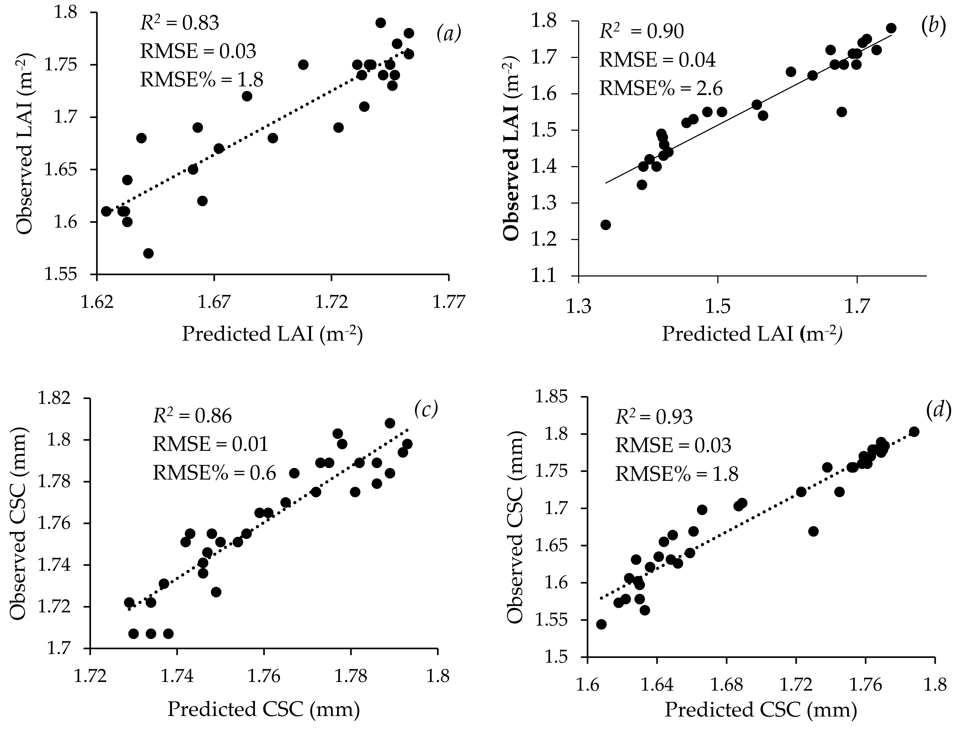
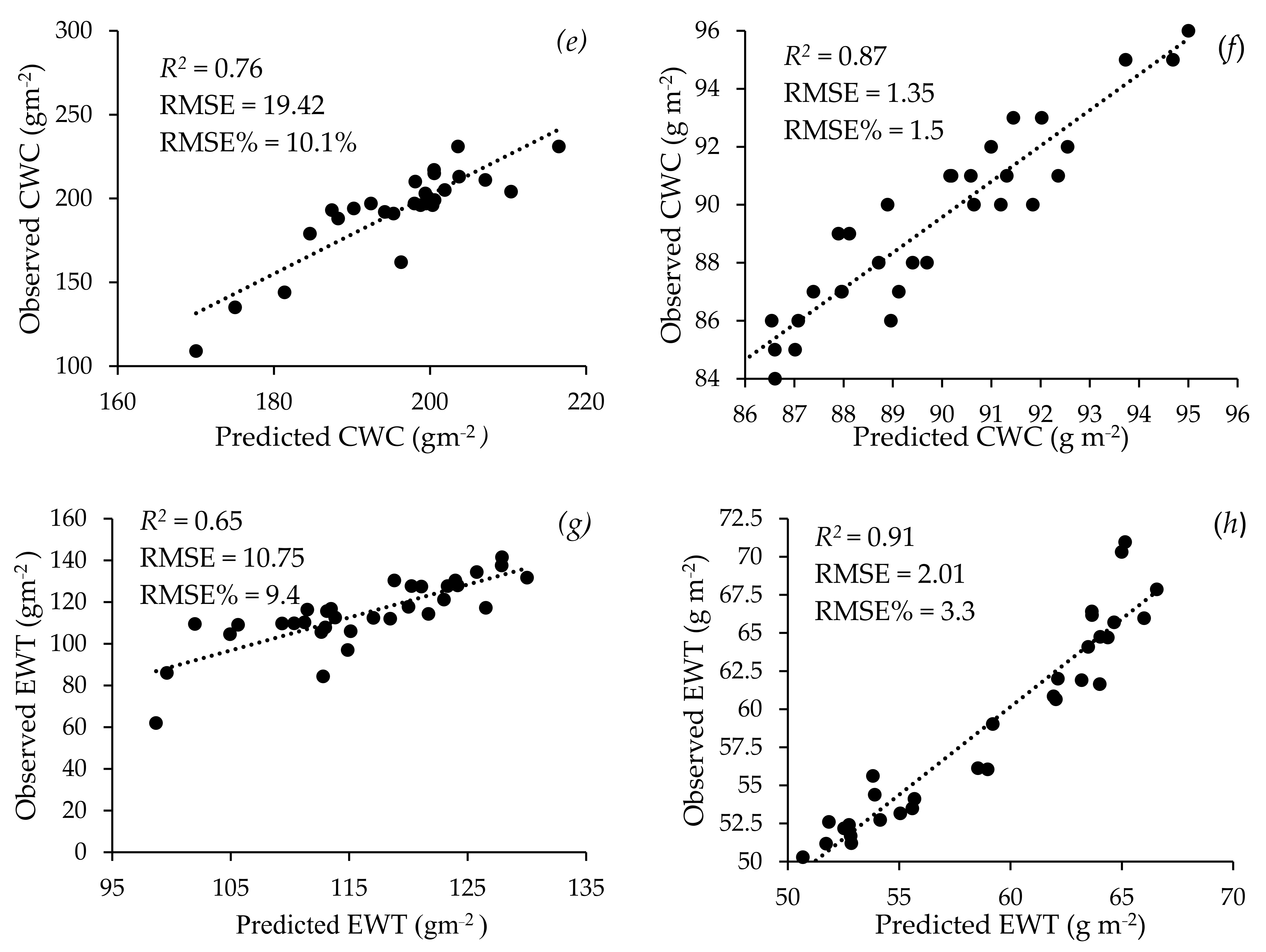
• The use of multisource data in conjunction with RF in the GEE can be used to model the LAI, CSC, CWC, and EWT with acceptable accuracies. The LAI was best estimated in the wet season with an accuracy of RMSE = 0.03 m⁻² and R² = 0.83 as compared to the dry season (RMSE = 0.04 m⁻² and R² = 0.90). Similarly, CSC was estimated with a high accuracy in the wet seasons, yielding an RMSE of 0.01 mm and R² of 0.86, compared to the dry season (RMSE = 0.03 mm and R² = 0.93). For CWC, the wet season results show an RMSE of 19.42 g/m⁻² and R² of 0.76, which were lower than those obtained for the dry season (RMSE = 1.35 g/m⁻² and R² = 0.87). Finally, EWT was best estimated in the dry season (RMSE = 2.01 g/m⁻² and R² = 0.91) as compared to the wet season (RMSE = 10.75 g/m⁻² and R² = 0.65).
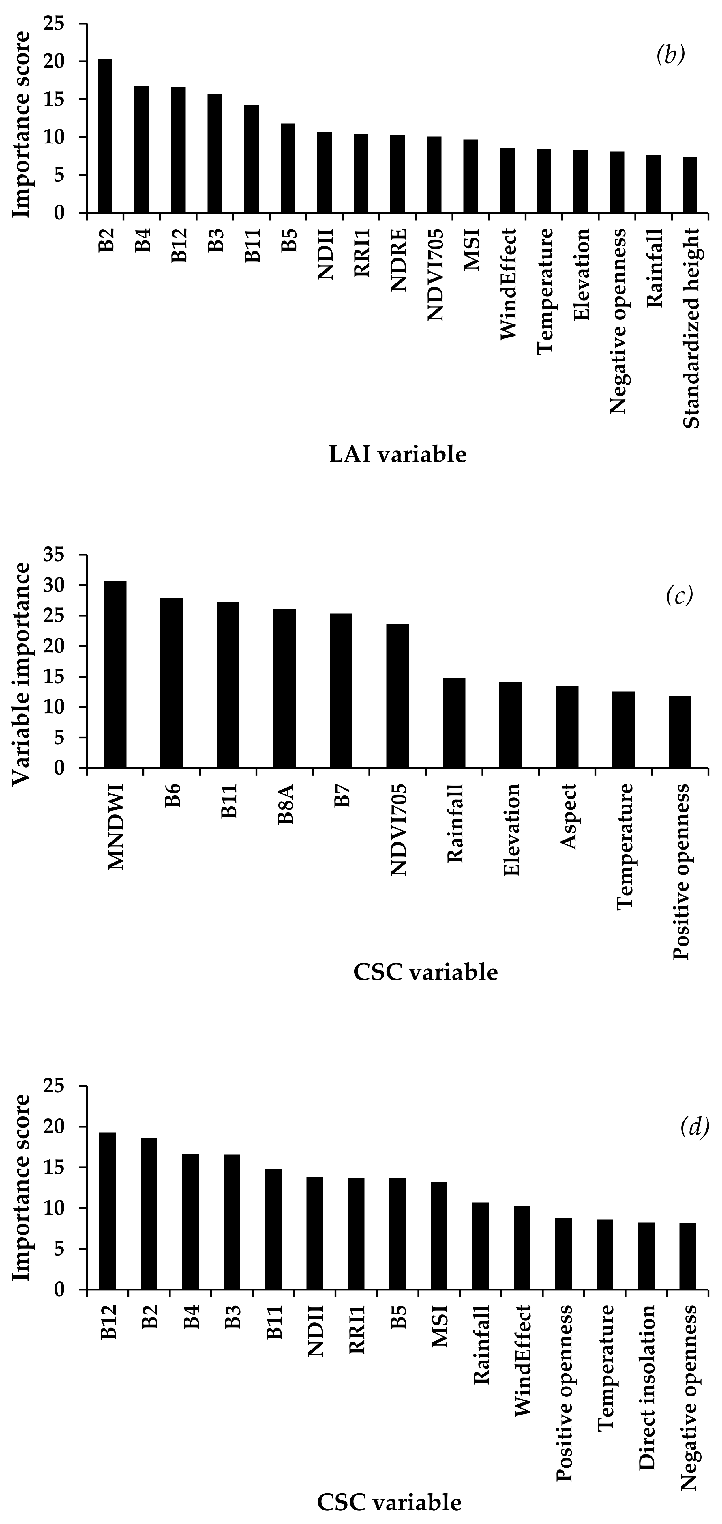
• The optimal model for estimating the LAI (RMSE of 0.03 m⁻² and R² of 0.83) had MNDWI, B7, B6, B11, B8A, B8, NDWI, Minimum curvature, Rainfall, Positive openness, Temperature, and Direct insolation as the optimal predictor variables.
• Overall, CSC performed optimally as an indicator of grass water content across both seasons based on MNDWI, B6, B11, B8A, B7, NDVI705, Rainfall, Elevation, Aspect, Temperature, and Positive openness in the wet season and B12, B2, B4, B3, B11, NDII, RR1, B5, MSI, Rainfall, Wind effect, Positive openness, Temperature, Direct insolation, and Negative openness in the dry season.
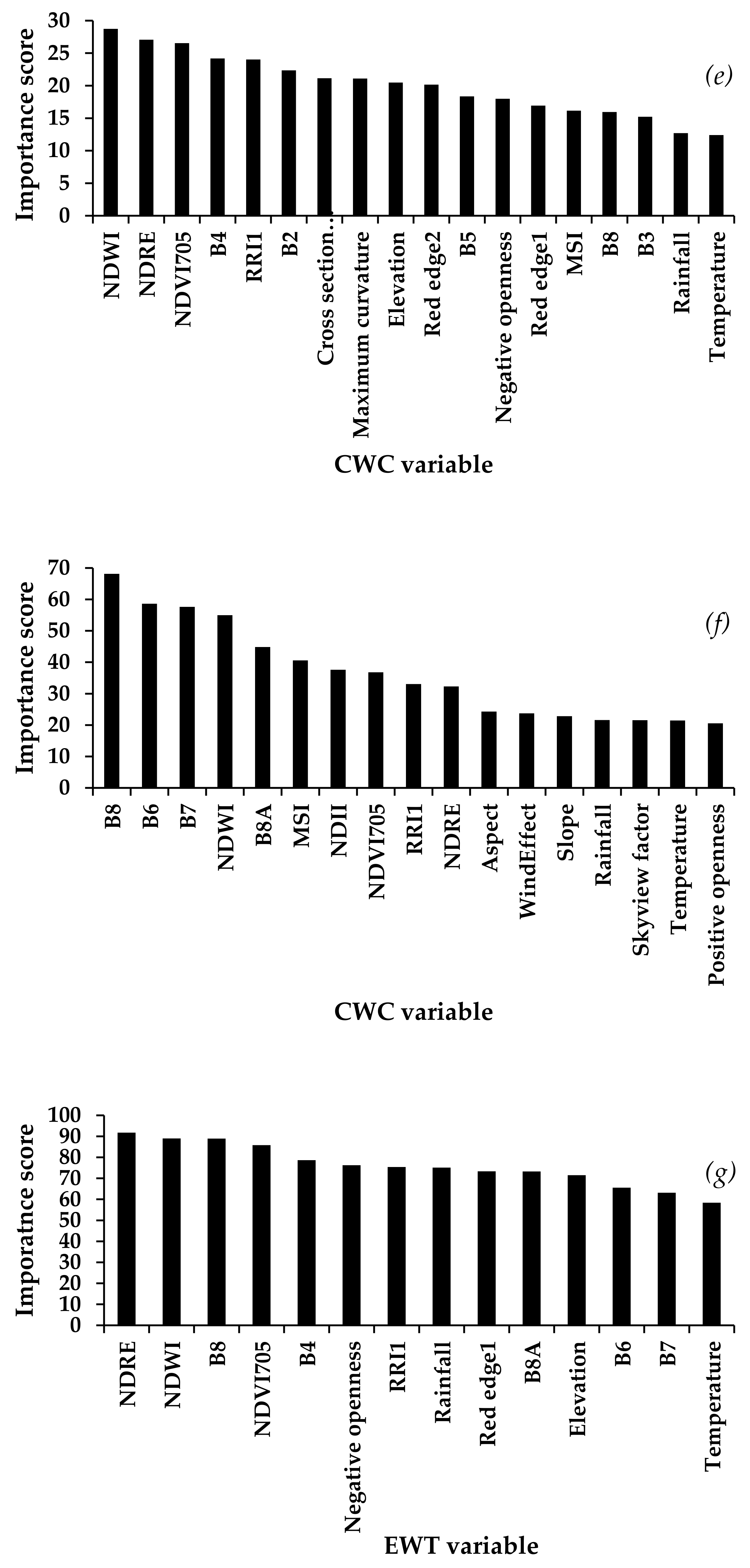
• CWC was best estimated in the dry season based on B8, B6, B7, NDWI, B8A, MSI, NDII, NDVI705, RRI1, NDRE, Aspect, Wind effect, Slope, Rainfall, Skyview factor, Temperature, and Positive openness as the optimal predictor variables, also in order of importance.
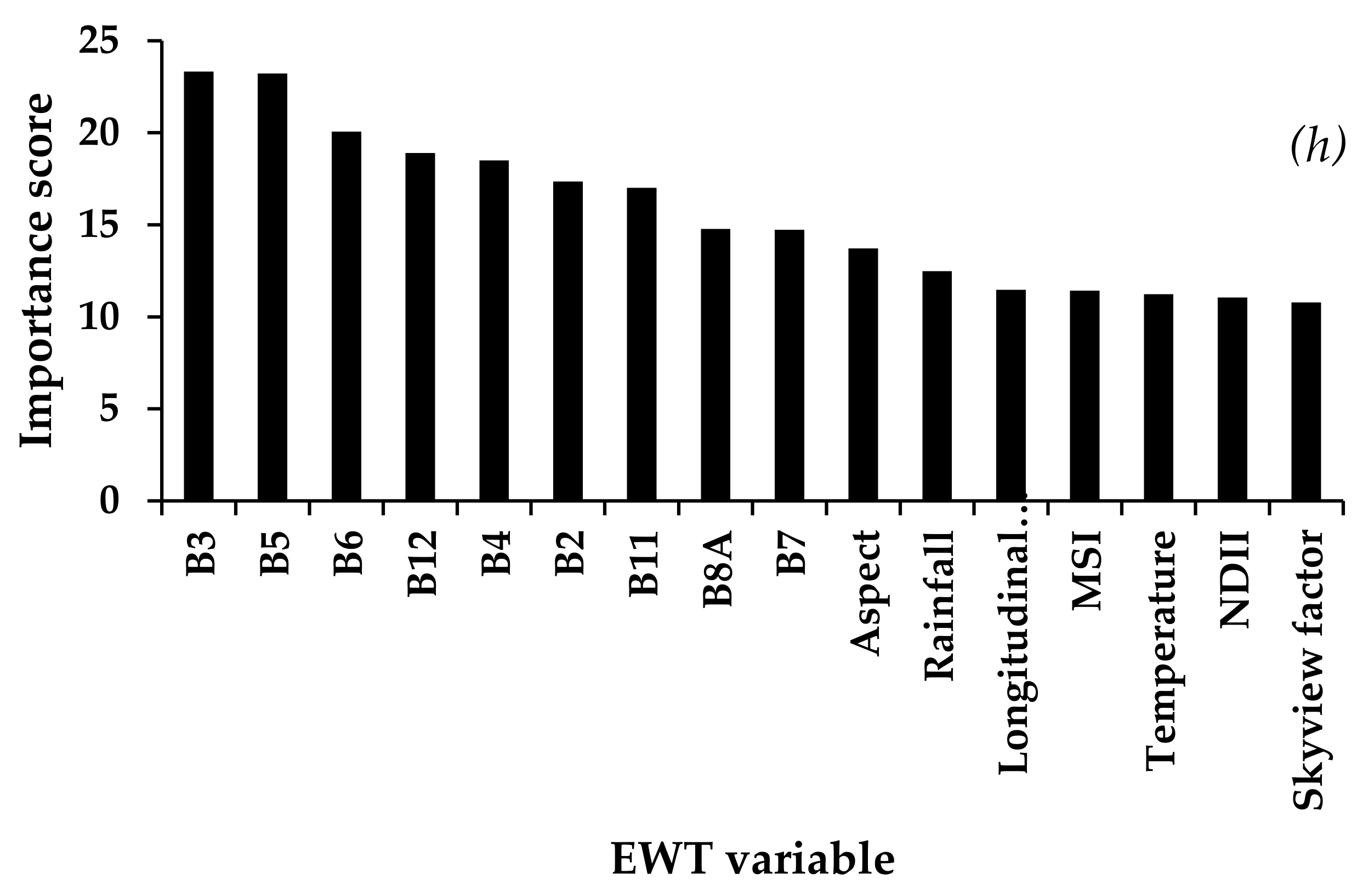
• EWT was estimated with high accuracies in the dry season using B3, B5, B6, B12, B4, B2, B11, B8A, B7, Aspect, Rainfall, Longitudinal curvature, MSI, Temperature, NDII, and Skyview factor as optimal predictor variables.

References

1. Koike, T.; Nakamura, Y.; Kaihotsu, I.; Davaa, G.; Matsuura, N.; Tamagawa, K.; Fujii, H. Development of an advanced microwave scanning radiometer (AMSR-E) algorithm for soil moisture and vegetation water content. Proc. Hydraul. Eng. 2004, 48, 217–222. [Google Scholar] [CrossRef] [Green Version]
2. Osakabe, Y.; Osakabe, K.; Shinozaki, K.; Tran, L.-S.P. Response of plants to water stress. Front. Plant Sci. 2014, 5, 86. [Google Scholar] [CrossRef] [PubMed] [Green Version]
3. Bonan, G.B. Forests and climate change: Forcings, feedbacks, and the climate benefits of forests. Science 2008, 320, 1444–1449. [Google Scholar] [CrossRef] [PubMed] [Green Version]
4. Cervena, L.; Lhotakova, Z.; Kupkova, L.; Kovarova, M.; Albrechtova, J. Models for estimating leaf pigments and relative water content in three vertical canopy levels of Norway spruce based on laboratory spectroscopy. In Proceedings of the 34th EARSeL Symposium, Warsaw, Poland, 16–20 June 2014. [Google Scholar] [CrossRef]
5. Browne, M.; Yardimci, N.T.; Scoffoni, C.; Jarrahi, M.; Sack, L. Prediction of leaf water potential and relative water content using terahertz radiation spectroscopy. Plant Direct 2020, 4, e00197. [Google Scholar] [CrossRef]
6. Ferreira, L.G.; Asner, G.P.; Knapp, D.E.; Davidson, E.A.; Coe, M.; Bustamante, M.M.; de Oliveira, E.L. Equivalent water thickness in savanna ecosystems: MODIS estimates based on ground and EO-1 Hyperion data. Int. J. Remote Sens. 2011, 32, 7423–7440. [Google Scholar] [CrossRef]
7. Zhu, L.; Webb, G.I.; Yebra, M.; Scortechini, G.; Miller, L.; Petitjean, F. Live fuel moisture content estimation from MODIS: A deep learning approach. ISPRS J. Photogramm. Remote Sens. 2021, 179, 81–91. [Google Scholar] [CrossRef]
8. Ustin, S.L.; Riaño, D.; Hunt, E.R. Estimating canopy water content from spectroscopy. Isr. J. Plant Sci. 2012, 60, 9–23. [Google Scholar] [CrossRef] [Green Version]
9. Zhou, S.; Duursma, R.A.; Medlyn, B.E.; Kelly, J.W.; Prentice, I.C. How should we model plant responses to drought? An analysis of stomatal and non-stomatal responses to water stress. Agric. For. Meteorol. 2013, 182, 204–214. [Google Scholar] [CrossRef]
10. Bulcock, H.; Jewitt, G. Spatial mapping of leaf area index using hyperspectral remote sensing for hydrological applications with a particular focus on canopy interception. Hydrol. Earth Syst. Sci. 2010, 14, 383–392. [Google Scholar] [CrossRef] [Green Version]
11. Sibanda, M.; Mutanga, O.; Dube, T.; Vundla, T.S.; Mafongoya, P.L. Estimating LAI and mapping canopy storage capacity for hydrological applications in wattle infested ecosystems using Sentinel-2 MSI derived red edge bands. GIScience Remote Sens. 2019, 56, 68–86. [Google Scholar] [CrossRef]
12. Sibanda, M.; Mutanga, O.; Dube, T.; Mabhaudhi, T. Quantitative assessment of grassland foliar moisture parameters as an inference on rangeland condition in the mesic rangelands of southern Africa. Int. J. Remote Sens. 2021, 42, 1474–1491. [Google Scholar] [CrossRef]
13. Pan, H.; Chen, Z.; Ren, J.; Li, H.; Wu, S. Modeling winter wheat leaf area index and canopy water content with three different approaches using Sentinel-2 multispectral instrument data. IEEE J. Sel. Top. Appl. Earth Obs. Remote Sens. 2018, 12, 482–492. [Google Scholar] [CrossRef]
14. Gao, Z.; Wang, Q.; Cao, X.; Gao, W. The responses of vegetation water content (EWT) and assessment of drought monitoring along a coastal region using remote sensing. GIScience Remote Sens. 2014, 51, 1–16. [Google Scholar] [CrossRef]
15. Zhang, F.; Zhou, G. Estimation of vegetation water content using hyperspectral vegetation indices: A comparison of crop water indicators in response to water stress treatments for summer maize. BMC Ecol. 2019, 19, 18. [Google Scholar] [CrossRef] [Green Version]
16. Ndlovu, H.S.; Odindi, J.; Sibanda, M.; Mutanga, O.; Clulow, A.; Chimonyo, V.G.P.; Mabhaudhi, T. A comparative estimation of maize leaf water content using machine learning techniques and unmanned aerial vehicle (UAV)-based proximal and remotely sensed data. Remote Sens. 2021, 13, 4091. [Google Scholar] [CrossRef]
17. Chuvieco, E.; Riaño, D.; Aguado, I.; Cocero, D. Estimation of fuel moisture content from multitemporal analysis of Landsat Thematic Mapper reflectance data: Applications in fire danger assessment. Int. J. Remote Sens. 2002, 23, 2145–2162. [Google Scholar] [CrossRef]
18. Danson, F.M.; Bowyer, P. Estimating live fuel moisture content from remotely sensed reflectance. Remote Sens. Environ. 2004, 92, 309–321. [Google Scholar] [CrossRef]
19. Oumar, Z.; Mutanga, O. Predicting plant water content in Eucalyptus grandis forest stands in KwaZulu-Natal, South Africa using field spectra resampled to the Sumbandila Satellite Sensor. Int. J. Appl. Earth Obs. Geoinf. 2010, 12, 158–164. [Google Scholar] [CrossRef]
20. Gómez-Giráldez, P.J.; Aguilar, C.; Polo, M.J. Natural vegetation covers as indicators of the soil water content in a semiarid mountainous watershed. Ecol. Indic. 2014, 46, 524–535. [Google Scholar] [CrossRef]
21. Zhang, J.; Xu, Y.; Yao, F.; Wang, P.; Guo, W.; Li, L.; Yang, L. Advances in estimation methods of vegetation water content based on optical remote sensing techniques. Sci. China Technol. Sci. 2010, 53, 1159–1167. [Google Scholar] [CrossRef]
22. Rubio, M.; Riaño, D.; Cheng, Y.; Ustin, S. Estimation of canopy water content from MODIS using artificial neural networks trained with radiative transfer models. Proceedings of 6th Annual Meeting of the European Meteorological Society & 6th European Conference on Applied Climatology, Ljubljana, Slovenia, 4–8 September 2006. [Google Scholar]
23. Wang, L.-T.; Wang, S.-X.; Zhou, Y.; Liu, W.-L.; Wang, F.-T. Vegetation water content retrieval and application of drought monitoring using multi-spectral remote sensing. Guang Pu Xue Yu Guang Pu Fen Xi Guang Pu 2011, 31, 2804–2808. [Google Scholar] [PubMed]
24. Yilmaz, M.T.; Hunt, E.R., Jr.; Goins, L.D.; Ustin, S.L.; Vanderbilt, V.C.; Jackson, T.J. Vegetation water content during SMEX04 from ground data and Landsat 5 Thematic Mapper imagery. Remote Sens. Environ. 2008, 112, 350–362. [Google Scholar] [CrossRef] [Green Version]
25. Clevers, J.G.; Kooistra, L.; Schaepman, M.E.; Liang, S.; Groot, N.E.; Kneubühler, M. Canopy Water Content Retrieval from Hyperspectral Remote Sensing. Proceedings of ISPRS Working Group VII/1 Workshop ISPMSRS’07: “Physical Measurements and Signatures in Remote Sensing”, Davos, Switzerland, 12–14 March 2007. [Google Scholar]
26. Neinavaz, E.; Skidmore, A.K.; Darvishzadeh, R.; Groen, T.A. Retrieving vegetation canopy water content from hyperspectral thermal measurements. Agric. For. Meteorol. 2017, 247, 365–375. [Google Scholar] [CrossRef]
27. Lehnert, L.W.; Meyer, H.; Wang, Y.; Miehe, G.; Thies, B.; Reudenbach, C.; Bendix, J. Retrieval of grassland plant coverage on the Tibetan Plateau based on a multi-scale, multi-sensor and multi-method approach. Remote Sens. Environ. 2015, 164, 197–207. [Google Scholar] [CrossRef]
28. Quemada, C.; Pérez-Escudero, J.M.; Gonzalo, R.; Ederra, I.; Santesteban, L.G.; Torres, N.; Iriarte, J.C. Remote Sensing for Plant Water Content Monitoring: A Review. Remote Sens. 2021, 13, 2088. [Google Scholar] [CrossRef]
29. Roberto, C.; Lorenzo, B.; Michele, M.; Micol, R.; Cinzia, P. 10 Optical Remote Sensing of Vegetation Water Content. In Hyperspectral Indices and Image Classifications for Agriculture and Vegetation; Thenkabail, P.S., Lyon, J.G., Huete, A., Eds.; CRC Press: Boca Raton, FL, USA, 2016; p. 227. ISBN 9781439845387. [Google Scholar]
30. Zhang, F.; Zhou, G. Research progress on monitoring vegetation water content by using hyperspectral remote sensing. Chin. J. Plant Ecol. 2018, 42, 517–525. [Google Scholar] [CrossRef]
31. Zhang, T.; Su, J.; Liu, C.; Chen, W.-H.; Liu, H.; Liu, G. Band selection in Sentinel-2 satellite for agriculture applications. In Proceedings of the 2017 23rd International Conference on Automation and Computing (ICAC), Huddersfield, UK, 7–8 September 2017; pp. 1–6. [Google Scholar]
32. Bramich, J.; Bolch, C.J.; Fischer, A. Improved red-edge chlorophyll-a detection for Sentinel 2. Ecol. Indic. 2021, 120, 106876. [Google Scholar] [CrossRef]
33. Zhou, H.; Zhou, G.; Song, X.; He, Q. Dynamic characteristics of canopy and vegetation water content during an entire maize growing season in relation to spectral-based indices. Remote Sens. 2022, 14, 584. [Google Scholar] [CrossRef]
34. Ceccato, P.; Flasse, S.; Tarantola, S.; Jacquemoud, S.; Grégoire, J.-M. Detecting vegetation leaf water content using reflectance in the optical domain. Remote Sens. Environ. 2001, 77, 22–33. [Google Scholar] [CrossRef]
35. Ghulam, A.; Li, Z.-L.; Qin, Q.; Tong, Q.; Wang, J.; Kasimu, A.; Zhu, L. A method for canopy water content estimation for highly vegetated surfaces-shortwave infrared perpendicular water stress index. Sci. China Ser. D: Earth Sci. 2007, 50, 1359–1368. [Google Scholar] [CrossRef]
36. Zeng, N.; Ren, X.; He, H.; Zhang, L.; Zhao, D.; Ge, R.; Li, P.; Niu, Z. Estimating grassland aboveground biomass on the Tibetan Plateau using a random forest algorithm. Ecol. Indic. 2019, 102, 479–487. [Google Scholar] [CrossRef]
37. Zhou, W.; Li, H.; Xie, L.; Nie, X.; Wang, Z.; Du, Z.; Yue, T. Remote sensing inversion of grassland aboveground biomass based on high accuracy surface modeling. Ecol. Indic. 2021, 121, 107215. [Google Scholar] [CrossRef]
38. Emran, A.; Roy, S.; Bagmar, M.S.H.; Mitra, C. Assessing topographic controls on vegetation characteristics in Chittagong Hill Tracts (CHT) from remotely sensed data. Remote Sens. Appl. Soc. Environ. 2018, 11, 198–208. [Google Scholar] [CrossRef]
39. Odebiri, O.; Mutanga, O.; Odindi, J.; Peerbhay, K.; Dovey, S.; Ismail, R. Estimating soil organic carbon stocks under commercial forestry using topo-climate variables in KwaZulu-Natal, South Africa. S. Afr. J. Sci. 2020, 116, 1–8. [Google Scholar] [CrossRef] [Green Version]
40. Mouillot, F.; Rambal, S.; Joffre, R. Simulating climate change impacts on fire frequency and vegetation dynamics in a Mediterranean-type ecosystem. Glob. Chang. Biol. 2002, 8, 423–437. [Google Scholar] [CrossRef]
41. Zeppel, M.; Wilks, J.V.; Lewis, J.D. Impacts of extreme precipitation and seasonal changes in precipitation on plants. Biogeosciences 2014, 11, 3083–3093. [Google Scholar] [CrossRef] [Green Version]
42. Mutanga, O.; Kumar, L. Google Earth Engine Applications. Remote Sens. 2019, 11, 591. [Google Scholar] [CrossRef] [Green Version]
43. Amani, M.; Ghorbanian, A.; Ahmadi, S.A.; Kakooei, M.; Moghimi, A.; Mirmazloumi, S.M.; Moghaddam, S.H.A.; Mahdavi, S.; Ghahremanloo, M.; Parsian, S.; et al. Google Earth Engine Cloud Computing Platform for Remote Sensing Big Data Applications: A Comprehensive Review. IEEE J. Sel. Top. Appl. Earth Obs. Remote Sens. 2020, 13, 5326–5350. [Google Scholar] [CrossRef]
44. Kumar, L.; Mutanga, O. Google Earth Engine applications since inception: Usage, trends, and potential. Remote Sens. 2018, 10, 1509. [Google Scholar] [CrossRef] [Green Version]
45. Martin-Ortega, P.; Garcia-Montero, L.G.; Sibelet, N. Temporal Patterns in Illumination Conditions and Its Effect on Vegetation Indices Using Landsat on Google Earth Engine. Remote Sens. 2020, 12, 211. [Google Scholar] [CrossRef] [Green Version]
46. Pérez-Cutillas, P.; Pérez-Navarro, A.; Conesa-García, C.; Zema, D.A.; Amado-Álvarez, J.P. What is going on within google earth engine? A systematic review and meta-analysis. Remote Sens. Appl. Soc. Environ. 2023, 29, 100907. [Google Scholar] [CrossRef]
47. Alexakis, D.D.; Manoudakis, S.; Agapiou, A.; Polykretis, C. Towards the Assessment of Soil-Erosion-Related C-Factor on European Scale Using Google Earth Engine and Sentinel-2 Images. Remote Sens. 2021, 13, 5019. [Google Scholar] [CrossRef]
48. Stefanidis, S.; Alexandridis, V.; Mallinis, G. A cloud-based mapping approach for assessing spatiotemporal changes in erosion dynamics due to biotic and abiotic disturbances in a Mediterranean Peri-Urban forest. CATENA 2022, 218, 106564. [Google Scholar] [CrossRef]
49. Long, T.; Zhang, Z.; He, G.; Jiao, W.; Tang, C.; Wu, B.; Zhang, X.; Wang, G.; Yin, R. 30 m resolution global annual burned area mapping based on Landsat Images and Google Earth Engine. Remote Sens. 2019, 11, 489. [Google Scholar] [CrossRef] [Green Version]
50. Seydi, S.T.; Akhoondzadeh, M.; Amani, M.; Mahdavi, S. Wildfire damage assessment over Australia using sentinel-2 imagery and MODIS land cover product within the google earth engine cloud platform. Remote Sens. 2021, 13, 220. [Google Scholar] [CrossRef]
51. Li, H.; Luo, Z.; Xu, Y.; Zhu, S.; Chen, X.; Geng, X.; Xiao, L.; Wan, W.; Cui, Y. A remote sensing-based area dataset for approximately 40 years that reveals the hydrological asynchrony of Lake Chad based on Google Earth Engine. J. Hydrol. 2021, 603, 126934. [Google Scholar] [CrossRef]
52. Fu, B.; Lan, F.; Xie, S.; Liu, M.; He, H.; Li, Y.; Liu, L.; Huang, L.; Fan, D.; Gao, E.; et al. Spatio-temporal coupling coordination analysis between marsh vegetation and hydrology change from 1985 to 2019 using LandTrendr algorithm and Google Earth Engine. Ecol. Indic. 2022, 137, 108763. [Google Scholar] [CrossRef]
53. Liu, X.; Zhai, H.; Shen, Y.; Lou, B.; Jiang, C.; Li, T.; Hussain, S.B.; Shen, G. Large-Scale Crop Mapping From Multisource Remote Sensing Images in Google Earth Engine. IEEE J. Sel. Top. Appl. Earth Obs. Remote Sens. 2020, 13, 414–427. [Google Scholar] [CrossRef]
54. Amani, M.; Kakooei, M.; Moghimi, A.; Ghorbanian, A.; Ranjgar, B.; Mahdavi, S.; Davidson, A.; Fisette, T.; Rollin, P.; Brisco, B. Application of google earth engine cloud computing platform, sentinel imagery, and neural networks for crop mapping in Canada. Remote Sens. 2020, 12, 3561. [Google Scholar] [CrossRef]
55. Li, Q.; Qiu, C.; Ma, L.; Schmitt, M.; Zhu, X.X. Mapping the Land Cover of Africa at 10 m Resolution from Multi-Source Remote Sensing Data with Google Earth Engine. Remote Sens. 2020, 12, 602. [Google Scholar] [CrossRef] [Green Version]
56. Xie, S.; Liu, L.; Zhang, X.; Yang, J.; Chen, X.; Gao, Y. Automatic Land-Cover Mapping using Landsat Time-Series Data based on Google Earth Engine. Remote Sens. 2019, 11, 3023. [Google Scholar] [CrossRef] [Green Version]
57. Reza Pahlefi, M.; Danoedoro, P.; Kamal, M. The utilisation of sentinel-2A images and google earth engine for monitoring tropical Savannah grassland. Geocarto Int. 2022, 37, 5400–5414. [Google Scholar] [CrossRef]
58. Reyes-Muñoz, P.; Pipia, L.; Salinero-Delgado, M.; Belda, S.; Berger, K.; Estévez, J.; Morata, M.; Rivera-Caicedo, J.P.; Verrelst, J. Quantifying Fundamental Vegetation Traits over Europe Using the Sentinel-3 OLCI Catalogue in Google Earth Engine. Remote Sens. 2022, 14, 1347. [Google Scholar] [CrossRef]
59. Municipality, M. Vulindlela Local Area Plan: Spatial Framework; Msunduzi Municipality: Pietermaritzburg, South African, 2016. [Google Scholar]
60. Alcock, P.G.; Verster, E. An assessment of water-quality in the inadi ward, vulindlela district, kwazulu. Water SA 1987, 13, 215–224. [Google Scholar]
61. Royimani, L.; Mutanga, O.; Odindi, J.; Slotow, R. Multi-Temporal Assessment of Remotely Sensed Autumn Grass Senescence across Climatic and Topographic Gradients. Land 2023, 12, 183. [Google Scholar] [CrossRef]
62. Rouault, M.; Richard, Y. Intensity and spatial extension of drought in South Africa at different time scales. Water SA 2003, 29, 489–500. [Google Scholar] [CrossRef] [Green Version]
63. Ndlovu, M.S.; Demlie, M. Assessment of meteorological drought and wet conditions using two drought indices across KwaZulu-Natal Province, South Africa. Atmosphere 2020, 11, 623. [Google Scholar] [CrossRef]
64. Royimani, L.; Mutanga, O.; Odindi, J.; Sibanda, M.; Chamane, S. Determining the onset of autumn grass senescence in subtropical sour-veld grasslands using remote sensing proxies and the breakpoint approach. Ecol. Inform. 2022, 69, 101651. [Google Scholar] [CrossRef]
65. Fynn, R.; Morris, C.; Ward, D.; Kirkman, K. Trait–environment relations for dominant grasses in South African mesic grassland support a general leaf economic model. J. Veg. Sci. 2011, 22, 528–540. [Google Scholar] [CrossRef]
66. Tsvuura, Z.; Kirkman, K.P. Yield and species composition of a mesic grassland savanna in S outh A frica are influenced by long-term nutrient addition. Austral Ecol. 2013, 38, 959–970. [Google Scholar] [CrossRef]
67. Cho, M.A.; Onisimo, M.; Mabhaudhi, T. Using participatory GIS and collaborative management approaches to enhance local actors’ participation in rangeland management: The case of Vulindlela, South Africa. J. Environ. Plan. Manag. 2021, 1–20. [Google Scholar] [CrossRef]
68. Yan, G.; Hu, R.; Luo, J.; Weiss, M.; Jiang, H.; Mu, X.; Xie, D.; Zhang, W. Review of indirect optical measurements of leaf area index: Recent advances, challenges, and perspectives. Agric. For. Meteorol. 2019, 265, 390–411. [Google Scholar] [CrossRef]
69. Kozak, J.A.; Ahuja, L.R.; Green, T.R.; Ma, L. Modelling crop canopy and residue rainfall interception effects on soil hydrological components for semi-arid agriculture. Hydrol. Process. Int. J. 2007, 21, 229–241. [Google Scholar] [CrossRef]
70. Wang, Q.; Shi, W.; Li, Z.; Atkinson, P.M. Fusion of Sentinel-2 images. Remote Sens. Environ. 2016, 187, 241–252. [Google Scholar] [CrossRef] [Green Version]
71. Gascon, F.; Bouzinac, C.; Thépaut, O.; Jung, M.; Francesconi, B.; Louis, J.; Lonjou, V.; Lafrance, B.; Massera, S.; Gaudel-Vacaresse, A.; et al. Copernicus Sentinel-2A calibration and products validation status. Remote Sens. 2017, 9, 584. [Google Scholar] [CrossRef] [Green Version]
72. Jin, Z.; Azzari, G.; You, C.; Di Tommaso, S.; Aston, S.; Burke, M.; Lobell, D.B. Smallholder maize area and yield mapping at national scales with Google Earth Engine. Remote Sens. Environ. 2019, 228, 115–128. [Google Scholar] [CrossRef]
73. Sola, I.; García-Martín, A.; Sandonís-Pozo, L.; Álvarez-Mozos, J.; Pérez-Cabello, F.; González-Audícana, M.; Llovería, R.M. Assessment of atmospheric correction methods for Sentinel-2 images in Mediterranean landscapes. Int. J. Appl. Earth Obs. Geoinf. 2018, 73, 63–76. [Google Scholar] [CrossRef]
74. Gao, J. Quantification of grassland properties: How it can benefit from geoinformatic technologies? Int. J. Remote Sens. 2006, 27, 1351–1365. [Google Scholar] [CrossRef]
75. Drusch, M.; Del Bello, U.; Carlier, S.; Colin, O.; Fernandez, V.; Gascon, F.; Hoersch, B.; Isola, C.; Laberinti, P.; Martimort, P.; et al. Sentinel-2: ESA’s optical high-resolution mission for GMES operational services. Remote Sens. Environ. 2012, 120, 25–36. [Google Scholar] [CrossRef]
76. Wijewardana, C.; Alsajri, F.A.; Irby, J.T.; Krutz, L.J.; Golden, B.; Henry, W.B.; Gao, W.; Reddy, K.R. Physiological assessment of water deficit in soybean using midday leaf water potential and spectral features. J. Plant Interact. 2019, 14, 533–543. [Google Scholar] [CrossRef] [Green Version]
77. Sims, D.A.; Gamon, J.A. Estimation of vegetation water content and photosynthetic tissue area from spectral reflectance: A comparison of indices based on liquid water and chlorophyll absorption features. Remote Sens. Environ. 2003, 84, 526–537. [Google Scholar] [CrossRef]
78. Adamczyk, J.; Osberger, A. Red-edge vegetation indices for detecting and assessing disturbances in Norway spruce dominated mountain forests. Int. J. Appl. Earth Obs. Geoinf. 2015, 37, 90–99. [Google Scholar] [CrossRef]
79. Dong, T.; Liu, J.; Shang, J.; Qian, B.; Ma, B.; Kovacs, J.M.; Walters, D.; Jiao, X.; Geng, X.; Shi, Y. Assessment of red-edge vegetation indices for crop leaf area index estimation. Remote Sens. Environ. 2019, 222, 133–143. [Google Scholar] [CrossRef]
80. Gao, B.-C. NDWI-A normalized difference index for remote sensing of vegetation liquid water from space. Remote Sens. Environ. 1996, 52, 155–162. [Google Scholar] [CrossRef]
81. Xu, H. Modification of normalised difference water index (NDWI) to enhance open water features in remotely sensed imagery. Int. J. Remote Sens. 2006, 27, 3025–3033. [Google Scholar] [CrossRef]
82. Klemas, V.; Smart, R. The influence of soil salinity, growth form, and leaf moisture on-the spectral radiance of. Photogramm. Eng. Remote Sens. 1983, 49, 77–83. [Google Scholar]
83. Hunt, E.R., Jr.; Rock, B.N. Detection of changes in leaf water content using near-and middle-infrared reflectances. Remote Sens. Environ. 1989, 30, 43–54. [Google Scholar]
84. Barnes, E.; Clarke, T.; Richards, S.; Colaizzi, P.; Haberland, J.; Kostrzewski, M.; Waller, P.; Choi, C.; Riley, E.; Thompson, T. Coincident detection of crop water stress, nitrogen status and canopy density using ground based multispectral data. In Proceedings of the Fifth International Conference on Precision Agriculture, Bloomington, MN, USA, 16–19 July 2000; p. 6. [Google Scholar]
85. Ehammer, A.; Fritsch, S.; Conrad, C.; Lamers, J.; Dech, S. Statistical derivation of fPAR and LAI for irrigated cotton and rice in arid Uzbekistan by combining multi-temporal RapidEye data and ground measurements. In Remote Sensing for Agriculture, Ecosystems, and Hydrology XII; International Society for Optics and Photonics: Washington, DC, USA, 2010; p. 782409. [Google Scholar]
86. Cloutis, E.; Connery, D.; Major, D.; Dover, F. Airborne multi-spectral monitoring of agricultural crop status: Effect of time of year, crop type and crop condition parameter. Remote Sens. 1996, 17, 2579–2601. [Google Scholar] [CrossRef]
87. Gamon, J.; Surfus, J. Assessing leaf pigment content and activity with a reflectometer. New Phytol. 1999, 143, 105–117. [Google Scholar] [CrossRef]
88. Speight, J.G. Parametric description of land form. Land Eval. 1968, 239–250. [Google Scholar]
89. Young, A. Slopes, Oliver and Boyd, Edinburgh; Wetenschappen: Haarlem, The Netherlands, 1972. [Google Scholar]
90. Shary, P.; Kuryakova, G.; Florinsky, I. On the international experience of topographic methods employment in landscape researches (the concise review). Geom. Earth Surf. Struct. 1991, 15–29. [Google Scholar]
91. Moore, I.D.; Gessler, P.E.; Nielsen, G.; Peterson, G.A. Soil attribute prediction using terrain analysis. Soil Sci. Soc. Am. J. 1993, 57, 443–452. [Google Scholar] [CrossRef]
92. Gumede, N.; Mutanga, O.; Sibanda, M. Mapping leaf area index of the Yellowwood tree species in an Afromontane mistbelt forest of southern Africa using topographic variables. Remote Sens. Appl. Soc. Environ. 2022, 27, 100778. [Google Scholar] [CrossRef]
93. Breiman, L. Random forests. Mach. Learn. 2001, 45, 5–32. [Google Scholar] [CrossRef] [Green Version]
94. Duro, D.C.; Franklin, S.E.; Dubé, M.G. Multi-scale object-based image analysis and feature selection of multi-sensor earth observation imagery using random forests. Int. J. Remote Sens. 2012, 33, 4502–4526. [Google Scholar] [CrossRef]
95. Rodriguez-Galiano, V.; Sanchez-Castillo, M.; Chica-Olmo, M.; Chica-Rivas, M. Machine learning predictive models for mineral prospectivity: An evaluation of neural networks, random forest, regression trees and support vector machines. Ore Geol. Rev. 2015, 71, 804–818. [Google Scholar] [CrossRef]
96. Wang, L.a.; Zhou, X.; Zhu, X.; Dong, Z.; Guo, W. Estimation of biomass in wheat using random forest regression algorithm and remote sensing data. Crop J. 2016, 4, 212–219. [Google Scholar] [CrossRef] [Green Version]
97. Li, Z.-W.; Xin, X.-P.; Tang, H.; Yang, F.; Chen, B.-R.; Zhang, B.-H. Estimating grassland LAI using the Random Forests approach and Landsat imagery in the meadow steppe of Hulunber, China. J. Integr. Agric. 2017, 16, 286–297. [Google Scholar] [CrossRef]
98. Odebiri, O.; Mutanga, O.; Odindi, J.; Peerbhay, K.; Dovey, S. Predicting soil organic carbon stocks under commercial forest plantations in KwaZulu-Natal province, South Africa using remotely sensed data. GIScience Remote Sens. 2020, 57, 450–463. [Google Scholar] [CrossRef]
99. Belgiu, M.; Drăguţ, L. Random forest in remote sensing: A review of applications and future directions. ISPRS J. Photogramm. Remote Sens. 2016, 114, 24–31. [Google Scholar] [CrossRef]
100. Shataee, S.; Kalbi, S.; Fallah, A.; Pelz, D. Forest attribute imputation using machine-learning methods and ASTER data: Comparison of k-NN, SVR and random forest regression algorithms. Int. J. Remote Sens. 2012, 33, 6254–6280. [Google Scholar] [CrossRef]
101. Yuan, Q.; Li, S.; Yue, L.; Li, T.; Shen, H.; Zhang, L. Monitoring the variation of vegetation water content with machine learning methods: Point–surface fusion of MODIS products and GNSS-IR observations. Remote Sens. 2019, 11, 1440. [Google Scholar] [CrossRef] [Green Version]
102. Lu, B.; He, Y. Evaluating empirical regression, machine learning, and radiative transfer modelling for estimating vegetation chlorophyll content using bi-seasonal hyperspectral images. Remote Sens. 2019, 11, 1979. [Google Scholar] [CrossRef] [Green Version]
103. Elmahdy, S.I.; Ali, T.A.; Mohamed, M.M.; Howari, F.M.; Abouleish, M.; Simonet, D. Spatiotemporal mapping and monitoring of mangrove forests changes from 1990 to 2019 in the Northern Emirates, UAE using random forest, Kernel logistic regression and Naive Bayes Tree models. Front. Environ. Sci. 2020, 8, 102. [Google Scholar] [CrossRef]
104. Shen, B.; Ding, L.; Ma, L.; Li, Z.; Pulatov, A.; Kulenbekov, Z.; Chen, J.; Mambetova, S.; Hou, L.; Xu, D. Modeling the Leaf Area Index of Inner Mongolia Grassland Based on Machine Learning Regression Algorithms Incorporating Empirical Knowledge. Remote Sens. 2022, 14, 4196. [Google Scholar] [CrossRef]
105. Oshiro, T.M.; Perez, P.S.; Baranauskas, J.A. How many trees in a random forest. In International Workshop on Machine Learning and Data Mining in Pattern Recognition; Springer: Berlin/Heidelberg, Germany, 2012; pp. 154–168. [Google Scholar]
106. Singh, B.; Sihag, P.; Singh, K. Modelling of impact of water quality on infiltration rate of soil by random forest regression. Model. Earth Syst. Environ. 2017, 3, 999–1004. [Google Scholar] [CrossRef]
107. Masenyama, A.; Mutanga, O.; Dube, T.; Bangira, T.; Sibanda, M.; Mabhaudhi, T. A systematic review on the use of remote sensing technologies in quantifying grasslands ecosystem services. GIScience Remote Sens. 2022, 59, 1000–1025. [Google Scholar] [CrossRef]
108. Singh, L.; Mutanga, O.; Mafongoya, P.; Peerbhay, K. Remote sensing of key grassland nutrients using hyperspectral techniques in KwaZulu-Natal, South Africa. J. Appl. Remote Sens. 2017, 11, 036005. [Google Scholar] [CrossRef]
109. Ullah, S.; Si, Y.; Schlerf, M.; Skidmore, A.K.; Shafique, M.; Iqbal, I.A. Estimation of grassland biomass and nitrogen using MERIS data. Int. J. Appl. Earth Obs. Geoinf. 2012, 19, 196–204. [Google Scholar] [CrossRef]
110. Moriasi, D.N.; Arnold, J.G.; Van Liew, M.W.; Bingner, R.L.; Harmel, R.D.; Veith, T.L. Model evaluation guidelines for systematic quantification of accuracy in watershed simulations. Trans. ASABE 2007, 50, 885–900. [Google Scholar] [CrossRef]
111. Richter, K.; Hank, T.B.; Mauser, W.; Atzberger, C. Derivation of biophysical variables from Earth observation data: Validation and statistical measures. J. Appl. Remote Sens. 2012, 6, 063557. [Google Scholar] [CrossRef]
112. Shoko, C.; Mutanga, O.; Dube, T. Determining optimal new generation satellite derived metrics for accurate C3 and C4 grass species aboveground biomass estimation in South Africa. Remote Sens. 2018, 10, 564. [Google Scholar] [CrossRef] [Green Version]
113. Sibanda, M.; Gumende, N.; Mutanga, O. Estimating leaf area index of the Yellowwood tree (Podocarpus spp.) in an indigenous Southern African Forest, using Sentinel 2 Multispectral Instrument data and the Random Forest regression ensemble. Geocarto Int. 2022, 37, 6953–6974. [Google Scholar] [CrossRef]
114. Sakowska, K.; Juszczak, R.; Gianelle, D. Remote sensing of grassland biophysical parameters in the context of the Sentinel-2 satellite mission. J. Sens. 2016, 2016, 4612809. [Google Scholar] [CrossRef] [Green Version]
115. Ose, K.; Corpetti, T.; Demagistri, L. Multispectral satellite image processing. In Optical Remote Sensing of Land Surface; Elsevier: Amsterdam, The Netherlands, 2016; pp. 57–124. [Google Scholar]
116. Frampton, W.J.; Dash, J.; Watmough, G.; Milton, E.J. Evaluating the capabilities of Sentinel-2 for quantitative estimation of biophysical variables in vegetation. ISPRS J. Photogramm. Remote Sens. 2013, 82, 83–92. [Google Scholar] [CrossRef] [Green Version]
117. Datt, B. Remote sensing of water content in Eucalyptus leaves. Aust. J. Bot. 1999, 47, 909–923. [Google Scholar] [CrossRef]
118. Gao, Y.; Walker, J.P.; Allahmoradi, M.; Monerris, A.; Ryu, D.; Jackson, T.J. Optical sensing of vegetation water content: A synthesis study. IEEE J. Sel. Top. Appl. Earth Obs. Remote Sens. 2015, 8, 1456–1464. [Google Scholar] [CrossRef] [Green Version]
119. Clevers, J.G.; Kooistra, L.; Schaepman, M.E. Using spectral information from the NIR water absorption features for the retrieval of canopy water content. Int. J. Appl. Earth Obs. Geoinf. 2008, 10, 388–397. [Google Scholar] [CrossRef]
120. Serrano, L.; Ustin, S.L.; Roberts, D.A.; Gamon, J.A.; Penuelas, J. Deriving water content of chaparral vegetation from AVIRIS data. Remote Sens. Environ. 2000, 74, 570–581. [Google Scholar] [CrossRef]
121. Lin, S.; Li, J.; Liu, Q.; Li, L.; Zhao, J.; Yu, W. Evaluating the effectiveness of using vegetation indices based on red-edge reflectance from Sentinel-2 to estimate gross primary productivity. Remote Sens. 2019, 11, 1303. [Google Scholar] [CrossRef] [Green Version]
122. Gholizadeh, A.; Mišurec, J.; Kopačková, V.; Mielke, C.; Rogass, C. Assessment of red-edge position extraction techniques: A case study for norway spruce forests using hymap and simulated sentinel-2 data. Forests 2016, 7, 226. [Google Scholar] [CrossRef] [Green Version]
123. Roy, P. Spectral reflectance characteristics of vegetation and their use in estimating productive potential. In Proceedings/Indian Academy of Sciences; Springer: Berlin/Heidelberg, Germany, 1989; pp. 59–81. [Google Scholar]
124. Caturegli, L.; Matteoli, S.; Gaetani, M.; Grossi, N.; Magni, S.; Minelli, A.; Corsini, G.; Remorini, D.; Volterrani, M. Effects of water stress on spectral reflectance of bermudagrass. Sci. Rep. 2020, 10, 15055. [Google Scholar] [CrossRef]
125. Easterday, K.; Kislik, C.; Dawson, T.E.; Hogan, S.; Kelly, M. Remotely sensed water limitation in vegetation: Insights from an experiment with unmanned aerial vehicles (UAVs). Remote Sens. 2019, 11, 1853. [Google Scholar] [CrossRef] [Green Version]
126. Eitel, J.U.; Vierling, L.A.; Litvak, M.E.; Long, D.S.; Schulthess, U.; Ager, A.A.; Krofcheck, D.J.; Stoscheck, L. Broadband, red-edge information from satellites improves early stress detection in a New Mexico conifer woodland. Remote Sens. Environ. 2011, 115, 3640–3646. [Google Scholar] [CrossRef]
127. Zhao, D.; Huang, L.; Li, J.; Qi, J. A comparative analysis of broadband and narrowband derived vegetation indices in predicting LAI and CCD of a cotton canopy. ISPRS J. Photogramm. Remote Sens. 2007, 62, 25–33. [Google Scholar] [CrossRef]
128. Alexander, C.; Deák, B.; Heilmeier, H. Micro-topography driven vegetation patterns in open mosaic landscapes. Ecol. Indic. 2016, 60, 906–920. [Google Scholar] [CrossRef]
129. Lukyanchuk, K.; Kovalchuk, I.; Pidkova, O. Application of a remote sensing in monitoring of erosion processes. In Geoinformatics: Theoretical and Applied Aspects; European Association of Geoscientists & Engineers: Utrecht, The Netherlands, 2020. [Google Scholar]
130. Amatulli, G.; Domisch, S.; Tuanmu, M.-N.; Parmentier, B.; Ranipeta, A.; Malczyk, J.; Jetz, W. A suite of global, cross-scale topographic variables for environmental and biodiversity modeling. Sci. Data 2018, 5, 180040. [Google Scholar] [CrossRef] [Green Version]
Figure 1. Location of the study area.
Applsci 13 03117 g001
Figure 2. Research methodology work chart used on each GWC variable across wet and dry season.
Applsci 13 03117 g002
Figure 3. Relationship between observed and predicted grass LAI (a,b), CSC (c,d), CWC (e,f), and EWT (g,h) derived using optimal selected predictor variables for the wet and dry seasons, respectively.
Applsci 13 03117 g003aApplsci 13 03117 g003b
Figure 4. Variable importance scores of selected variables in estimating (a,b) LAI, (c,d) CSC, (e,f) CWC, and (g,h) EWT for wet and dry seasons, respectively.
Applsci 13 03117 g004aApplsci 13 03117 g004bApplsci 13 03117 g004cApplsci 13 03117 g004d
Figure 5. Spatial distribution of modelled LAI (a,b), CSC (c,d), CWC (e,f), and EWT (g,h) for the wet and dry seasons, respectively.
Applsci 13 03117 g005