Exploring the Capabilities of a Lightweight CNN Model in Accurately Identifying Renal Abnormalities: Cysts, Stones, and Tumors, Using LIME and SHAP

Abstract

Kidney abnormality is one of the major concerns in modern society, and it affects millions of people around the world. To diagnose different abnormalities in human kidneys, a narrow-beam x-ray imaging procedure, computed tomography, is used, which creates cross-sectional slices of the kidneys. Several deep-learning models have been successfully applied to computer tomography images for classification and segmentation purposes. However, it has been difficult for clinicians to interpret the model’s specific decisions and, thus, creating a “black box” system. Additionally, it has been difficult to integrate complex deep-learning models for internet-of-medical-things devices due to demanding training parameters and memory-resource cost. To overcome these issues, this study proposed (1) a lightweight customized convolutional neural network to detect kidney cysts, stones, and tumors and (2) understandable AI Shapely values based on the Shapley additive explanation and predictive results based on the local interpretable model-agnostic explanations to illustrate the deep-learning model. The proposed CNN model performed better than other state-of-the-art methods and obtained an accuracy of 99.52 ± 0.84% for K = 10-fold of stratified sampling. With improved results and better interpretive power, the proposed work provides clinicians with conclusive and understandable results.

1. Introduction

The kidney, an abdominal organ that filter waste and excess water from the blood, can developed abnormalities [1] that have a significant impact on health and affect over 10% of the worldwide population [2]. The exact causes and mechanisms of kidney abnormalities have yet to be fully understood [3], but research in recent years has identified a variety of genetic, environmental, and lifestyle factors that may contribute to their development [4]. The severe symptoms of kidney abnormalities include a pain in the side or back; blood in the urine; fatigue; and swelling in the legs and feet [5]. The most common kidney abnormalities that impair kidney function are the development of cysts, nephrolithiasis (kidney stones), and renal cell carcinoma (kidney tumor) [6]. Kidney stones are hard crystalline mineralized material that varies in size and is formed in the kidney or urinary tract. The complex phenotype of kidney stone disease is caused by the interplay of several genes, in conjunction with dietary and environmental variables [7]. Another urinary problem, a cyst, is a fluid-filled sac in the kidneys [8], whereas tumors are abnormal growths with symptoms such as abdominal pain, blood in the urine, and unexplained weight loss [9].

In the early stages, patients may not show any symptoms or signs of kidney abnormalities, as they are initially benign. However, if untreated, they can develop further and even become malignant. For early detection and treatment, pathology tests are frequently used, with imaging techniques including X-rays, computer tomography (CT), B-ultrasound devices, and magnetic resonance imaging (MRI) [10]. Ultrasound devices that use high-frequency sound waves and MRIs may not be suitable for patients with medical implants or conditions. CT scans are generally faster and provide detailed images of dense tissues, such as bones in the spine and skull [11].

Despite its limitations, such as non-standardized image acquisition [12]; the improper labeling of data collected; and regulatory barriers [13], deep-learning (DL) research has show a significant positive impact in radiology applications, such as reducing the workload of radiologists [14]; increasing medical access in developing countries and rural areas [15]; and improving diagnostic accuracy [16]. DL models have been applied for a wide range of concerns, such as COVID-19 [17], brain tumors [18], radiation therapy [19], blood clotting [20], heart diseases [21], liver cancer [22], fin-tech [23], intrusion detection [24], vibration signals [25], organic pollutant classification [26], agriculture [27], and steganography [28]. Recent research has shown that DL models can be used successfully for diagnosing kidney abnormalities [29,30,31,32,33]. However, in diagnosing kidney abnormalities, the lightweight models [33] have achieved low accuracy, as compared to the more complex models [29,30,31,32]. Therefore, a lightweight customized DL model could be considered as an alternative approach to achieve higher accuracy.

Meanwhile, explainable artificial intelligence (XAI) [34] is a pragmatic tool that accelerates the creation of predictive models with domain knowledge and increases the transparency of automatically generated prediction models in the medical sector [35,36], which has assisted in providing results that are understandable to humans [37]. We noted that most of the recent research defined the detection of kidney problems in terms of individual categories, including stones [38], tumors [39], and cysts [40]. However, the proposed study classified all three abnormalities using a single model, and it provided the following contributions.

• For diagnosing three different kidney abnormalities, a fully automated lightweight DL architecture was proposed. The model’s capability to identify stones, cysts, and tumors was improved by utilizing a well-designed, customized convolutional neural network (CNN).
• The proposed model had fewer model parameters, surpassing current approaches, and was able to locate the target area precisely, so that it could operate effectively with internet of medical things (IoMT)-enabled devices.
• The explanatory classification of the model was conducted using XAI algorithms, a local interpretable model-agnostic explanation (LIME), and a Shapley additive explanation (SHAP).
• An ablation study of the proposed model was performed on a chest X-ray dataset for the diagnosis of COVID-19, pneumonia, tuberculosis, and healthy records.

2. Related Works

2.1. Conventional Practices

Most studies on the classification of kidney abnormalities have employed a region-of-interest (ROI) localization and conventional image processing approaches [41]. By limiting the necessity for invasive and ionizing diuretic renography, Cerrolaza et al. [42] presented a computer-aided design method to build a connection between non-invasive, non-ionizing imaging modalities and renal function. A subset of 10 characteristics was chosen for the predictive variables (size, geometric curvature descriptors, etc.). Specificity results of 53% and 75%, respectively, for the logistic regression and support-vector-machine (SVM) classifier were attained by adjusting the probability decision thresholds. On a dataset of more than 200 ultrasound images, Raja et al. [43] employed k-means clustering and a histogram equalization to localize the kidney and retrieved the textural features of the segmented region for classification, with a sensitivity of 94.60%.

2.2. Machine-Learning Practices

Before adopting a probabilistic neural network (PNN), the authors of [44] employed image enhancement and Gaussian filtering to obtain better features, and they achieved a classification accuracy of 92.99%, a sensitivity of 88.04%, and a specificity of 97.33%, on 77 ultrasound images of kidney, which included 4 different classes (normal, cyst, calculi, and tumor). An automated identification system for renal disorders was built by Raja et al. [45], using a hybrid fuzzy neural network with feature extraction techniques for 36 features. In this work, 150 ultrasound images were utilized for training, and 78 images were used for testing. The suggested approach achieved an F1-score of 82.92%. Viswanath et al. [46] used ultrasound images to create a model to identify kidney stones, and they initially used a diffusion method to locate the kidney. Multi-layer perception (MLP) was utilized as a classifier for the characteristics retrieved from ROI. The suggested approach obtained an accuracy of 98.8% on a dataset of approximately 500 images.

2.3. Deep-Learning Approaches

For modeling an artificial intelligence (AI)-based diagnostic system for kidney disease, the authors of [29] independently generated 12,446 CT images of the whole abdomen via CT urogram. Resnet50, VGG16, and Inception v3 were used to achieve accuracy rates of 73.40%, 98.20%, and 99.30%, respectively. The results from the models were further explained with the GradCAM XAI approach. Ahmet et al. [33] endeavored to identify kidney cysts and stones using YOLO architectures, which were augmented with XAI features. The performance analysis included CT images from three categories, including 72 kidney cysts, 394 kidney stones, and 192 healthy kidneys. The results indicated that their YOLOv7 architecture design outperformed the YOLOv7 tiny architecture design, achieving a mAP50 of 0.85, a precision of 0.882, a sensitivity of 0.829, and an F1-score of 0.854. A study by Abdalbasit et al. [30] focused on identifying the three types of kidney abnormalities (stones, cysts, and tumors) using AI techniques on a dataset of over 12,000 CT images. A hybrid approach of pre-trained models and machine-learning algorithms was used, and the Densenet-201 model and random-forest classification yielded an accuracy rate of 99.44%. Venkatesan et al. [31] proposed a framework for classifying renal CT images as healthy or malignant using a pre-trained deep-learning approach. To improve its accuracy, they employed a threshold-filter-based pre-processing scheme to eliminate artifacts. The process included four stages: image collection, deep feature extraction, feature reduction and fusion, and binary classification through a fivefold cross-validation. Experimentation on CT images with and without artifacts showed the KNN classifier achieved 100% accuracy by using pre-processed images.Using a XResNet-50 model, Kadir et al. [32] automated the diagnosis of kidney stones (the presence of stones vs. no stones present) using coronal CT images. Each subject had distinct cross-sectional CT scans taken, yielding a total of 1799 images, and the results had a 96.82% accuracy rate for diagnosing kidney stones. Using the features extracted from ResNet-101, ShuffleNet, and MobileNet-v2, kidney ultrasound images were categorized by the authors of [47] using an SVM. The final predictions were generated using the majority-vote technique to achieve a maximum accuracy of 95.58%. While considering stones, cysts, hyper-echogenicity, space-occupying lesions, and hydro-nephrosis as abnormalities, Tsai et al. [48] collected 330 normal and 1269 abnormal pediatric renal images from a U.S. database.After performing the pre-processing tasks, the final linking layer of ResNet50 was redefined, and an accuracy of 92.9% was achieved. Though several studies have employed different DL approaches for better accuracy, they have primarily used DL models that consisted of more parameters, and they have not focused on improving the clarity and transparency of the result from DL models. The proposed work clearly showed the superiority of the customized model in terms of performance, clarity, and training parameters.

3. Materials and Methods

3.1. Data Collection and Pre-Processing

A publicly available dataset (3709 cysts; 5077 normal; 1377 stones; 2283 tumors) was used in this study. Using the picture archiving and communication system (PACS), the annotators [29] of the dataset gathered data from various hospitals in Dhaka, Bangladesh. The images were prepared from a batch of Digital Imaging and Communications in Medicine (DICOM) standardized records.

The coronal and axial cuts were selected from both contrast and non-contrast studies to create DICOM images of the ROI for each radiological finding. For better computational efficiency, pixels were re-scaled into the [0, 1] range, and each image was resized to 150 × 150 pixels.In order to maintain a percentage of samples for each class, stratified sampling was utilized the training-and-testing split results. Figure 1 shows the sample images for individual categories.

3.2. Proposed Framework

The proposed framework included a CNN model and an XAI-based explanation framework. The CNN model classified CT images into four categories (cyst, normal, stone, tumor). The visual representation of the proposed CNN model is shown in Figure 2.

3.2.1. CNN Model

The CNN proved its capacity to create an internal representation of the two-dimensional images, which enabled the model to represent specific locations and scales of various image features, using different elements of AI, including deep-fake [49], medicine [36,50], agriculture [51] etc.

In the proposed customized CNN model (Figure 3), all five convolution layers were followed by max-pooling layers. The results of the final max-pooling layers were flattened, followed by a drop-out layer as well as two dense layers. In addition, an L2 regularization (l2 = 0.0001) was used for the last two dense layers to eliminate sparse weighting [52]. In order to visualize the ROI in the CT images more effectively [53], a kernel size of $3\times 3$ was used. According to Sitaula et al. [54], an ideal stride value of 1 should be used to enhance the medical images, as a greater stride had overlooked the discriminating semantic regions; therefore, the same was used in this study. Furthermore, to prevent the network from over-fitting, the dropout layer was adjusted to 0.2. We concluded the model was lightweight, and the parameters of all the layers are shown in

Table 1. Total parameters (trainable and non-trainable) of the proposed CNN model. Variables F, K, S, and FLOP denote the filters, kernel size, stride, and floating-point operations, respectively.

S.N.	Layer Type	(F, K, S)	Output Shape	Parameters	FLOPs
1	Input	-	(150, 150, 3)	0	-
2	Conv2D + relu	(3, 3, 1)	(148, 148, 63)	1792	25,233,408
3	MaxPool2D (2)	-	(74, 74, 64)	0	296
4	Conv2D + relu	(3, 3, 1)	(72, 72, 64)	36,928	5,971,968
5	MaxPool2D (2)	-	(36, 36, 64)	0	144
6	Conv2D + relu	(3, 3, 1)	(34, 34, 64)	36,928	1,331,712
7	MaxPool2D (2)	-	(17, 17, 64)	0	68
8	Conv2D + relu	(3, 3, 1)	(15, 15, 64)	36,928	259,200
9	MaxPool2D (2)	-	(7, 7, 64)	0	28
10	Conv2D + relu	(3, 3, 1)	(5, 5, 64)	36,928	5760
11	MaxPool2D (2)	-	(2, 2, 64)	0	8
12	Flatten	-	256	0	131,072
13	dropout (0.2)	-	256	0	-
14	Dense + relu + l2 (0.0001)	-	128	32,896	65,536
15	Dense + Softmax + l2 (0.0001)	-	4	512	1024
Total parameters					182,916
Total FLOPs					33,000,224

.

3.2.2. Explainable AI

XAI demonstrated the black-box approach recognized in DL models and revealed the precise reasoning behind their predictions [55]. As the complexity of DL models has increased, XAI has become an important strategy, particularly in domains where critical decisions are needed, such as for medical image analysis [56]. Medical experts have been able to more easily understand the results of these DL models and use them to quickly and accurately diagnose cysts, normal growths, kidney stones, and tumors [57].Therefore, Shapley additive explanation (SHAP) and local interpretable model-agnostic explanation (LIME), two popular XAI algorithms, were specified in this study.

By normalizing the marginal feature values, SHAP assessed the influence of the model features. The scores exemplified the significance of each pixel on a predicted image and were used to substantiate their classification. To obtain the Shapley value, all potential combinations of characteristics of kidney abnormalities were used. Red pixels increased the likelihood of predicting a class once the Shapley values were converted into pixels, while blue pixels reduced the likelihood [58]. The Shapley values were generated by Equation (1).

$${\varphi }_i=\sum _{S\subseteq N\backslash \left\{i\right\}}\frac{\left|S\right|!(M-|S|-1)!}{M!}[f_x(S\cup \left\{i\right\})-f_x(S)]$$

(1)

where $f_x$ is the adjustment of the output by Shapely values for feature i. Feature $N,S$ is the subset of the features, and $\frac{\left|S\right|!(M-|S|-1)!}{M!}$ is the weighing factor that determined the number of permutations of the subset S are present. The predicted result, $f_x(S)$, was calculated using Equation (2).

$$f_x(S)=E\left[f(x)\right|x_S]$$

(2)

where each original trait replaced $(x_i)$, using SHAP, and a binary variable $z_i^{\prime }$ is replaced that represents whether $x_i$ is absent or present, as shown in Equation (3)

$$g(z^{\prime })={\varphi }_0+\sum _{i=1}^M{\varphi }_i{z}_i^{\prime }=\sum featureContribution+bias$$

(3)

where the primordial model $f(x)$, in Equation (3), $g(z^{\prime })$ is the local surrogate model, feature i is based on the result, and ${\varphi }_i$ assisted in understanding the model.

To interpret the representation of an instance being presented in a way that could be explained, $(x\in {\mathbb{R}}^d)$ using LIME, a binary vector $(x^{\prime }\in {\{0,1\}}^{d^{\prime }})$ represented the “absence” or “presence”, and a continuous patched super-pixel was considered. Having domain ${\{0,1\}}^{d^{\prime }}$ for the model $g\in G$ to display the conclusive representation, g determined the presence/absence of the accountable components. We found that all the components of $g\in G$ could not interpret the results, so $\Omega (g)$ was utilized to gauge the complication of the explanation.

In order to classify the sample as either cyst, normal, stone, or tumor, and to define the locality around x for the proposed model $f:{\mathbb{R}}^d\to \mathbb{R}$: if $f(x)$ is the probability of x, then ${\pi }_x(z)$ is used as a proximity measure between an instance from z to x. To define the locality ${\pi }_x$, $\Im (f,g,{\pi }_x)$, as a fidelity function, was used as a dimension to determine the amount of error generated by g when calculating f. In order to maximize the interpretations, $\Omega (g)$ was reduced to the absolute minimum, and the fidelity function was similarly decreased. Overall, LIME, as an explanation generator, is summarized in Equation (4).

$$\xi (x)=\underset{g\in G}{argmax}\Im (f,g,{\pi }_x)+\Omega (g)$$

(4)

3.2.3. Implementation Details

The proposed CNN model and XAI algorithms were implemented in Python (version 3.7) using Keras (version 2.5.0) and Tensorflow (version 2.5.0). We collaborated using Google Colab’s runtime NVIDIA K80 GPU with 12 GB of RAM.

With a ratio of 90:10 for each category, the dataset was divided into the training and testing sets, respectively.The final averaged performance of the CT dataset was reported using K = 10 [59] for the separate, random training/testing assignments. Early termination was applied after monitoring validation loss across three epochs, and 10% of the training data were reserved for validation to prevent the model from over-fitting during training.

4. Evaluation Metrics

Considering $T_P$, $T_N$, $F_P$, and $F_N$ represented true positive, true negative, false positive, and false negative, respectively, the precision $(\frac{T_P}{T_P+F_P})$, the recall $(\frac{T_P}{T_P+F_N})$, the F1-score $(2\times \frac{P\times R}{P+R})$, the accuracy $(\frac{T_P+T_N}{T_P+T_N+F_P+F_N})$, and the receiver-operating curve-area under the curve (ROC-AUC) were calculated.

5. Results and Discussion

5.1. CNN Results

Traditional statistical validation variables were taken into account, including model loss and accuracy for the training, and for the validation and test sets, the precision, the F1-score, and the recall.

For 15 epochs, every fold was set to terminate early using callbacks that monitored the validation loss for 3 epochs. After 10 folds, the model achieved an average training accuracy of 99.30 ± 0.18%, a validation accuracy of 99.39 ± 0.99% (Figure 4), a training loss of 0.0557 ± 0.07, and a validation loss of 0.0491 ± 0.06 (Figure 5). In addition, the average testing accuracy and testing loss were 99.52 ± 0.84% and 0.0291 ± 0.03, respectively (

Table 2. For K = 10 folds, this table represents the training, testing, and validation performance of the proposed model (after 15 epochs, in %): Training Accuracy (TrA),Training Loss (TrL), Validation Accuracy (VaA), Validation Loss (VaL), Test Accuracy (TsA), and Test Loss (TsL).

	K1	K2	K3	K4	K5	K6	K7	K8	K9	K10	Avg ($\mathit{\mu }\pm \mathit{\sigma }$)
TrA	99.33	99.64	99.04	99.31	99.31	99.22	99.64	99.5	99.43	99.24	99.30 ± 0.18
TrL	0.0321	0.0192	0.0445	0.0348	0.0352	0.0350	0.0223	0.2680	0.0335	0.0323	0.0557 ± 0.07
VaA	99.76	99.68	96.47	100	99.76	99.76	99.84	99.68	99.76	99.2	99.39 ± 0.99
VaL	0.0208	0.0192	0.1518	0.0118	0.169	0.0195	0.0142	0.0201	0.0195	0.0452	0.0491 ± 0.06
TsA	99.84	99.76	97.19	100	100	100	100	99.68	99.84	98.88	99.52 ± 0.84
TsL	0.0221	0.0164	0.1106	0.0018	0.0145	0.0131	0.0117	0.0208	0.0178	0.0621	0.0291 ± 0.03

). Figure 6 shows the ROC-AUC of the 10th fold. Since the AUC for all abnormalities was 1.00, the model could precisely differentiate all positive and negative classes. As the ROC curve depended upon the true-positive rate (TPR) and false-positive rate (FPR), the model prediction on the test data supported a very high TPR, reaching 100% of the AUC values.Consequently, these results showed that even for classes with non-uniform sample distributions, the suggested model was more reliable and consistent.

5.2. Descriptive Analysis from XAI

5.2.1. SHAP

Since it was difficult to directly interpret the mathematical behavior of the CNN model, XAI techniques were applied to the model [60]. Four results were illustrated by the SHAP results for each category (cyst, normal, stone, tumor).Testing images are shown on the left with a transparent gray background behind each explanation.

Red pixels are featured in the first explanation image in Figure 7 to increase the probability that a cyst would be predicted. The likelihood that the input image would be classified as normal, stone, or tumor decreased, since the second, third, and fourth explanations did not contain any red or blue pixels. In Figure 8, the red pixels are concentrated in the normal image, indicated the image was normal, whereas Figure 9 and Figure 10 were determined as stone and tumor, respectively.

5.2.2. LIME

Using the means and standard deviation from the training data, The LIME image explainer was used to extract numerical features and perturbations, as sampled from a normal (0, 1) image, and perform the inverse operations of mean-centering and scaling. The explainer was adjusted so that it calculated the first 100 features using simple linear iterative clustering (SLIC) [61] to define the highest contributing boundaries and embed them in the image. The second column of

Table 3. LIME Result Interpretation along with Masked and Segmented Images.

Category	CT Image	Mask	LIME (Segmented)
Cyst
Normal
Stone
Tumor

shows the original test images for each category; these results defined the masks in the third column of Table 3. In the fourth column of Table 3, the segmented image portion, resulting from the mask, reflected the LIME results.

As shown in Table 3, LIME provided a visual explanation of the model’s decision-making process and highlighted the regions of the image that contributed significantly to a specific class prediction. For example, in Table 3, the segmented LIME results showed only those portions of the image that contributed to the image being classified as a cyst.

5.3. Class-Wise Study of Proposed CNN Model

In order to analyze the performance of the suggested model for each class of abnormalities, the precision (99.30 ± 1.55%–99.70 ± 0.64%), the recall (97.90 ± 3.30%–99.90 ± 0.30%), and the F1-score (98.8 ± 1.83%–99.80 ± 0.40%) were measured for 10 folds (

Table 4. K = 10-fold average result of the proposed model in (%): Precision (Pre), Recall (Rec), F1-score (Fsc).

		K1	K2	K3	K4	K5	K6	K7	K8	K9	K10	Avg ($\mathit{\mu }\pm \mathit{\sigma }$)
Pre	Cyst	99	99	99	100	100	100	100	100	99	98	99.4 ± 0.66
	Normal	100	100	97	100	100	100	100	99	100	100	99.5 ± 0.95
	Stone	100	100	98	100	100	100	100	99	100	100	99.7 ± 0.64
	Tumor	100	100	95	100	100	100	100	100	100	98	99.3 ± 1.55
Rec	Cyst	100	100	99	100	100	100	100	100	100	100	99.9 ± 0.30
	Normal	100	100	98	100	100	100	100	100	100	99	99.7 ± 0.64
	Stone	99	99	90	100	100	100	100	99	99	93	97.9 ± 3.30
	Tumor	100	100	96	100	100	100	100	99	100	100	99.5 ± 1.20
Fsc	Cyst	100	100	99	100	100	100	100	100	100	99	99.8 ± 0.40
	Normal	100	100	97	100	100	100	100	100	100	100	99.7 ± 0.89
	Stone	100	99	94	100	100	100	100	99	99	97	98.8 ± 1.83
	Tumor	100	100	96	100	100	100	100	100	100	99	99.5 ± 1.20

). The foremost F1-score for the cyst class was recorded by the proposed model, demonstrating the model’s superior ability to detect and recognize cysts. As all three categories had an F1-score greater than 98%, the model was also successful in detecting the normal, stone, and tumor categories. In addition, Figure 11 displays the confusion matrix for the correct and incorrect categorizations generated by the model.

5.4. Calculating the Floating-Point Operation

The floating-point operation (FLOPs) of the proposed model was computed for the total number of addition, subtraction, division, multiplication, or any other operation that requires a floating-point value. The total operations performed by the model were (33,000,224 operations), and this was calculated from the convolutional layers ($2\times NumberOfKernel$$\times KernelShape\times OutputShape$), the max-pooling layers ($Height\times Depth\times WidthOfImage$), and the fully connected layers ($2\times InputSize\times OutputSize$ ) and is shown in Table 1 in detail. The proposed model performed significantly fewer operations, only 33 million, as compared to other transfer-learning approaches using SOTA methods, such as InceptionV3 (6 billion) [62], VGG19 (19.6 billion) [63], and ResNet50 (3.8 billion) [64].

5.5. Comparison with the State-of-the-Art Methods

A comparative analysis with other state-of-the-art methods is shown in

Table 5. Comparative table for proposed model and other state-of-the-art models. Note: ‘Ev.P’, ‘P.M’, ‘TsA’, ‘Pre’, ‘Fs’, ‘AP’, ‘AR’ and ‘AF’ stand for evaluation protocol, parameters in millions, test accuracy, precision, F1-score, average precision, average recall, and average F1-score.

Ref.	Plane	Ev.P	Class	Model	Result		P.M	XAI
[29]	Coronal, Axial	64:16:20 10-fold	Normal—1300 Stone—1300 Cyst—1300 Tumor—1300	Inception v3	TsA	61.60%	22.32	GradCAM
				VGG16		98.20%	14.74
				Resnet		73.80%	23.71
				EANet		77.02%	6
				Swin Transformers		99.30%	4.12
				CCT		96.54%	4.07
[30]	Coronal, Axial and Sagittal	80:20:00	Normal—1350 Stone—1350 Cyst—1350 Tumor—1350	Densenet201- Random Forest	TsA	99.44%	20	N/A
[31]	Axial	80:10:10 5-fold	Normal—1340 Tumor—1340	VGG16-NB	TsA	96.26%	14.74	N/A
				Densenet121-KNN		96.64%	20
				VGG-DN-KNN		100.00%	14.74
[32]	coronal	80:20	Normal: 1009 Stone: 790	XResNet-50	TsA	96.82%	23.7	N/A
[33]	Axial	75:10:15	Normal—288 Stone—494 Cyst—498	YOLOv7	Pre.	88.20%	6	GradCAM
					Fs	85.40%
				YOLOv7 Tiny	Pre.	88.20%
					Fs.	85.40%
Ours	Coronal, Axial	80:10:10 10-fold	Cyst: 3709 Normal: 5077 Stone: 1377 Tumor: 2283	Custom CNN	TsA	99.39%	0.18	LIME SHAP
					AP	99.47%
					AR	99.25%
					AF	99.45%

, in terms of classes, results, and the number of parameters. All compared models used a transfer-learning approach with a high number of parameters, whereas the proposed model was a lightweight customized CNN and had significantly fewer parameters.

The authors of [29] classified 4 classes with an accuracy ranging from 61% to 99.30% for 6 different algorithms, and among them, CCT had the lowest number of parameters, at approximately 4.07 million. Our model achieved an accuracy of 99.52% with only 0.18 million parameters. Using only the axial plane for 3 different classes, the authors of [33] implemented 2 transfer-learning algorithms with approximately 6 million parameters. Both the algorithms achieved an approximately 85% precision and F1-score, whereas our model achieved more than 99%. With the same 3 different kidney planes for 4 classes, 99.44% was achieved by the authors of [30]. They used a DenseNet algorithm, and their model had 19.82 million more parameters than our model. Though the results obtained by VGG–DN–KNN using 5-fold cross-validation was 100% in the work performed by the authors of [31], it only achieved approximately 96% for VGG16–NB and Densenet121–KNN. All the algorithms implemented had a high number of parameters. The author of [32] applied XResNet50 to coronal images and achieved only 96.82% with 23.7 million parameters, whereas the proposed model had only 0.18 million parameters and achieved 99.52%.

6. Result Analysis: Medical Opinion

To enhance the confidence and trust in DL models, the interpretation and explanation of the DL models are required. This can only improve by testing DL models, including ours, on real-world samples and verifying the results with a medical expert [65].

6.1. Reception by Medical Professionals

Our results and the study’s CT images were presented to medical professionals and their views and medical opinions were records. The impressions of the medical professionals were then validated with the results of DL and XAI frameworks.

Table 6. Medical Sensation: Findings and Impressions.

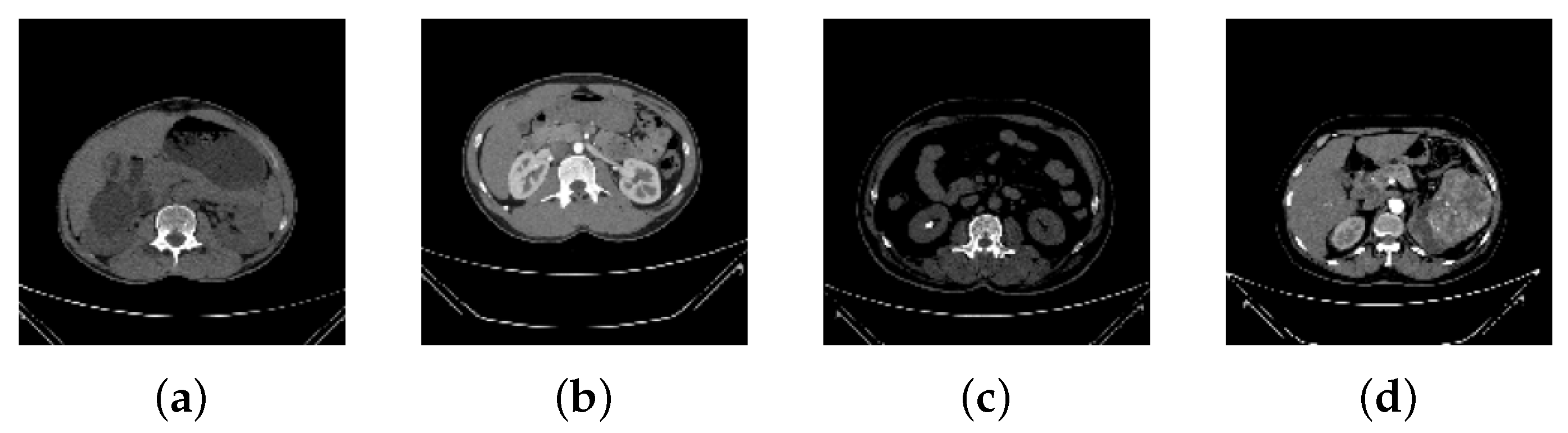
CT Image	Radiological Findings	Impressions
Figure 2a	Simple cystic lesion arising from right renal pelvis.	Right parapelvic cyst.
Figure 2b	Both kidneys appear normal in size; parenchyma shows normal width and structure.	Normal-appearing bilateral kidneys in the given section.
Figure 2c	Radiopaque lesion visualized in right kidney.	Right renal calculus.
Figure 2d	Heterogeneously enhancing lesion likely originating from left kidney.	Malignant mass arising from left kidney.

shows the overall feedback indicated the proposed study could effectively be utilized to identify kidney abnormalities in patients. To conclude, the proposed methodology could assist medical teams in making more accurate diagnoses and treatments.

6.2. Expert’s View towards to Dataset

CT images from the dataset were provided to medical experts for validation. The medical experts responded that the findings could be incomplete due to the absence of complete cross-sectional images of the individual organs.

7. Ablation Study of the Proposed Model

Ablation studies are crucial for deep-learning research [66]. Therefore, we adapted the dataset as chest X-ray (CXR) scans without any modification of the model, and we conducted an ablation study of the model to confirm its efficacy. A dataset [36] of 7132 CXR images in four categories, including COVID-19 (576), pneumonia (4273), tuberculosis (TB), and normal (1583), were ablated.

Since the dataset was imbalanced due to an insignificant amount of COVID-19 and TB data, a stratified sampling was utilized, and each image was scaled to 150 × 150 and [0, 1], correspondingly. The training, testing, and validation sets were randomly selected from the dataset according to a ratio of 80:10:10, respectively.

For 15 epochs, the callbacks were monitored for losses for 3 epochs. The 10-fold result of the model is shown in

Table 7. The 10-fold training, testing and validation results of the proposed model in CXR dataset (after 15 epochs, in %): Training Accuracy (TrA),Training Loss (TrL), Validation Accuracy (VaA), Validation Loss (VaL), Test Accuracy (TsA) and Test Loss (TsL).

	K1	K2	K3	K4	K5	K6	K7	K8	K9	K10	Avg ($\mathit{\mu }\pm \mathit{\sigma }$)
TrA	96.22	95.60	96.36	95.59	96.50	96.30	95.60	96.42	95.93	96.20	96.07 ± 0.34
TrL	0.1094	0.1360	0.1058	0.1278	0.1048	0.1120	0.1340	0.1589	0.1894	0.1012	0.1279 ± 0.03
VaA	95.93	92.85	94.53	92.99	94.24	95.22	92.91	94.41	94.13	94.78	94.20 ± 0.97
VaL	0.1281	0.1919	0.1804	0.2398	0.1964	0.2109	0.2034	0.2078	0.265	0.1831	0.2007 ± 0.03
TsA	94.26	89.92	94.40	92.30	94.54	94.30	93.12	94.55	93.30	94.36	93.50 ± 1.39
TsL	0.2009	0.2684	0.1618	0.2219	0.1589	0.1789	0.245	0.2719	0.2930	0.1680	0.2160 ± 0.047

. The model achieved a 96.07 ± 0.34% training accuracy, a 0.1279 ± 0.03 training loss, a 94.20 ± 0.97% validation accuracy, a 0.2007 ± 0.03 validation loss, a 93.50 ± 1.39% test accuracy, and a 0.2160 ± 0.047 test loss.

The confusion matrix of the 10th fold is shown in Figure 12. Only 5 COVID-19, 9 Normal, 15 pneumonia, and 10 TB images were misclassified, out of 69, 155, 423, and 67 images, respectively. Figure 13 shows the ROC-AUC curve that indicated the model supported the accurate diagnosis of COVID-19 and pneumonia.

According to the results of the ablation study, the model could be applied to CXR pictures in order to diagnose conditions such as COVID-19, normal, TB, and pneumonia.

8. Conclusions

This work presented a lightweight CNN architecture with XAI frameworks for categorizing four types of kidney abnormalities, including cyst, normal, tumor, and stone. The model achieved 99.30 ± 0.18%, 99.39 ± 0.99%, and 99.52 ± 0.84% accuracy for training, validation, and testing, respectively.The explanations provided by the XAI algorithms were verified by radiologists. Despite its lighter design, as compared to other state-of-art techniques, the model performed better in categorizing CT images of kidneys. The XAI results showed the model had the potential to be used as a support tool for IoMT devices. The ablation study showed that the model was more accurate for predicting COVID-19, normal, TB, and pneumonia conditions based on CXR images. This work used a limited number of CT samples, and the performance could be improved with data augmentation. The transparency of the results could be improved by combining DL models with other XAI algorithms. However, as the model negated aggregate characteristics, such as medical histories, experience gaps, and other physical signs, human supervision is still required.

References

- Pyeritz, R.E. Renal Tubular Disorders. In Emery and Rimoin’s Principles and Practice of Medical Genetics and Genomics; Elsevier: Amsterdam, The Netherlands, 2023; pp. 115–124. [Google Scholar]
- Kovesdy, C.P. Epidemiology of chronic kidney disease: An update 2022. Kidney Int. Suppl. 2022, 12, 7–11. [Google Scholar] [CrossRef]
- Maynar, J.; Barrasa, H.; Martin, A.; Usón, E.; Fonseca, F. Kidney Support in Sepsis. In The Sepsis Codex-E-Book; Elsevier Health Sciences: Amsterdam, The Netherlands, 2023; p. 169. [Google Scholar]
- Li, M.; Chi, X.; Wang, Y.; Setrerrahmane, S.; Xie, W.; Xu, H. Trends in insulin resistance: Insights into mechanisms and therapeutic strategy. Signal Transduct. Target. Ther. 2022, 7, 216. [Google Scholar] [CrossRef]
- Yener, S.; Pehlivanoğlu, C.; Yıldız, Z.A.; Ilce, H.T.; Ilce, Z. Duplex Kidney Anomalies and Associated Pathologies in Children: A Single-Center Retrospective Review. Cureus 2022, 14, e25777. [Google Scholar] [CrossRef]
- Sassanarakkit, S.; Hadpech, S.; Thongboonkerd, V. Theranostic roles of machine learning in clinical management of kidney stone disease. Comput. Struct. Biotechnol. J. 2022, 21, 260–266. [Google Scholar] [CrossRef]
- Kanti, S.Y.; Csóka, I.; Jójárt-Laczkovich, O.; Adalbert, L. Recent Advances in Antimicrobial Coatings and Material Modification Strategies for Preventing Urinary Catheter-Associated Complications. Biomedicines 2022, 10, 2580. [Google Scholar] [CrossRef]
- Ramalingam, H.; Patel, V. Decorating Histones in Polycystic Kidney Disease. J. Am. Soc. Nephrol. 2022, 33, 1629–1630. [Google Scholar] [CrossRef]
- Karimi, K.; Nikzad, M.; Kulivand, S.; Borzouei, S. Adrenal Mass in a 70-Year-Old Woman. Case Rep. Endocrinol. 2022, 2022, 2736199. [Google Scholar] [CrossRef] [PubMed]
- Saw, K.C.; McAteer, J.A.; Monga, A.G.; Chua, G.T.; Lingeman, J.E.; Williams, J.C., Jr. Helical CT of urinary calculi: Effect of stone composition, stone size, and scan collimation. Am. J. Roentgenol. 2000, 175, 329–332. [Google Scholar] [CrossRef]
- Park, H.J.; Kim, S.Y.; Singal, A.G.; Lee, S.J.; Won, H.J.; Byun, J.H.; Choi, S.H.; Yokoo, T.; Kim, M.J.; Lim, Y.S. Abbreviated magnetic resonance imaging vs. ultrasound for surveillance of hepatocellular carcinoma in high-risk patients. Liver Int. 2022, 42, 2080–2092. [Google Scholar] [CrossRef]
- Ahmad, S.; Nan, F.; Wu, Y.; Wu, Z.; Lin, W.; Wang, L.; Li, G.; Wu, D.; Yap, P.T. Harmonization of Multi-site Cortical Data across the Human Lifespan. In Machine Learning in Medical Imaging, Proceedings of the 13th International Workshop, MLMI 2022, Singapore, 18 September 2022; Springer: Cham, Switzerland, 2022; pp. 220–229. [Google Scholar]
- Mezrich, J.L. Is Artificial Intelligence (AI) a Pipe Dream? Why Legal Issues Present Significant Hurdles to AI Autonomy. Am. J. Roentgenol. 2022, 219, 152–156. [Google Scholar] [CrossRef]
- European Society of Radiology (ESR). Current practical experience with artificial intelligence in clinical radiology: A survey of the European Society of Radiology. Insights Into Imaging 2022, 13, 107. [Google Scholar] [CrossRef] [PubMed]
- Bazoukis, G.; Hall, J.; Loscalzo, J.; Antman, E.M.; Fuster, V.; Armoundas, A.A. The inclusion of augmented intelligence in medicine: A framework for successful implementation. Cell Rep. Med. 2022, 3, 100485. [Google Scholar] [CrossRef]
- van Leeuwen, K.G.; de Rooij, M.; Schalekamp, S.; van Ginneken, B.; Rutten, M.J. How does artificial intelligence in radiology improve efficiency and health outcomes? Pediatr. Radiol. 2022, 52, 2087–2093. [Google Scholar] [CrossRef]
- Jungmann, F.; Müller, L.; Hahn, F.; Weustenfeld, M.; Dapper, A.K.; Mähringer-Kunz, A.; Graafen, D.; Düber, C.; Schafigh, D.; Pinto dos Santos, D.; et al. Commercial AI solutions in detecting COVID-19 pneumonia in chest CT: Not yet ready for clinical implementation? Eur. Radiol. 2022, 32, 3152–3160. [Google Scholar] [CrossRef]
- Islam, K.T.; Wijewickrema, S.; O’Leary, S. A Deep Learning Framework for Segmenting Brain Tumors Using MRI and Synthetically Generated CT Images. Sensors 2022, 22, 523. [Google Scholar] [CrossRef] [PubMed]
- Charyyev, S.; Wang, T.; Lei, Y.; Ghavidel, B.; Beitler, J.J.; McDonald, M.; Curran, W.J.; Liu, T.; Zhou, J.; Yang, X. Learning-based synthetic dual energy CT imaging from single energy CT for stopping power ratio calculation in proton radiation therapy. Br. J. Radiol. 2022, 95, 20210644. [Google Scholar] [CrossRef]
- Mirakhorli, F.; Vahidi, B.; Pazouki, M.; Barmi, P.T. A Fluid-Structure Interaction Analysis of Blood Clot Motion in a Branch of Pulmonary Arteries. Cardiovasc. Eng. Technol. 2022; ahead of print. [Google Scholar]
- Lozano, P.F.R.; Kaso, E.R.; Bourque, J.M.; Morsy, M.; Taylor, A.M.; Villines, T.C.; Kramer, C.M.; Salerno, M. Cardiovascular Imaging for Ischemic Heart Disease in Women: Time for a Paradigm Shift. JACC Cardiovasc. Imaging 2022, 15, 1488–1501. [Google Scholar] [CrossRef]
- Araújo, J.D.L.; da Cruz, L.B.; Diniz, J.O.B.; Ferreira, J.L.; Silva, A.C.; de Paiva, A.C.; Gattass, M. Liver segmentation from computed tomography images using cascade deep learning. Comput. Biol. Med. 2022, 140, 105095. [Google Scholar] [CrossRef]
- Khanal, M.; Khadka, S.R.; Subedi, H.; Chaulagain, I.P.; Regmi, L.N.; Bhandari, M. Explaining the Factors Affecting Customer Satisfaction at the Fintech Firm F1 Soft by Using PCA and XAI. FinTech 2023, 2, 70–84. [Google Scholar] [CrossRef]
- Chapagain, P.; Timalsina, A.; Bhandari, M.; Chitrakar, R. Intrusion Detection Based on PCA with Improved K-Means. In Innovations in Electrical and Electronic Engineering; Mekhilef, S., Shaw, R.N., Siano, P., Eds.; Springer: Singapore, 2022; pp. 13–27. [Google Scholar]
- Chen, H.Y.; Lee, C.H. Deep Learning Approach for Vibration Signals Applications. Sensors 2021, 21, 3929. [Google Scholar] [CrossRef]
- Molinara, M.; Cancelliere, R.; Di Tinno, A.; Ferrigno, L.; Shuba, M.; Kuzhir, P.; Maffucci, A.; Micheli, L. A Deep Learning Approach to Organic Pollutants Classification Using Voltammetry. Sensors 2022, 22, 8032. [Google Scholar] [CrossRef]
- Bhandari, M.; Shahi, T.B.; Neupane, A.; Walsh, K.B. BotanicX-AI: Identification of Tomato Leaf Diseases using Explanation-driven Deep Learning Model. J. Imaging 2023, 9, 53. [Google Scholar] [CrossRef] [PubMed]
- Bhandari, M.; Panday, S.; Bhatta, C.P.; Panday, S.P. Image Steganography Approach Based Ant Colony Optimization with Triangular Chaotic Map. In Proceedings of the 2022 2nd International Conference on Innovative Practices in Technology and Management (ICIPTM), Gautam Buddha Nagar, India, 23–25 February 2022; Volume 2, pp. 429–434. [Google Scholar] [CrossRef]
- Islam, M.N.; Hasan, M.; Hossain, M.; Alam, M.; Rabiul, G.; Uddin, M.Z.; Soylu, A. Vision transformer and explainable transfer learning models for auto detection of kidney cyst, stone and tumor from CT-radiography. Sci. Rep. 2022, 12, 11440. [Google Scholar] [CrossRef] [PubMed]
- Qadir, A.M.; Abd, D.F. Kidney Diseases Classification using Hybrid Transfer-Learning DenseNet201-Based and Random Forest Classifier. Kurd. J. Appl. Res. 2023, 7, 131–144. [Google Scholar] [CrossRef]
- Rajinikanth, V.; Durai Raj Vincent, P.M.; Srinivasan, K.; Ananth Prabhu, G.; Chang, C.Y. Framework to Distinguish Healthy/Cancer Renal CT Images using Fused Deep Features. Front. Public Health 2023, 11, 39. [Google Scholar] [CrossRef]
- Yildirim, K.; Bozdag, P.G.; Talo, M.; Yildirim, O.; Karabatak, M.; Acharya, U.R. Deep learning model for automated kidney stone detection using coronal CT images. Comput. Biol. Med. 2021, 135, 104569. [Google Scholar] [CrossRef]
- Bayram, A.F.; Gurkan, C.; Budak, A.; Karataş, H. A Detection and Prediction Model Based on Deep Learning Assisted by Explainable Artificial Intelligence for Kidney Diseases. Avrupa Bilim Teknol. Derg. 2022, 40, 67–74. [Google Scholar]
- Loveleen, G.; Mohan, B.; Shikhar, B.S.; Nz, J.; Shorfuzzaman, M.; Masud, M. Explanation-Driven HCI Model to Examine the Mini-Mental State for Alzheimer’s Disease. ACM Trans. Multimed. Comput. Commun. Appl. 2022. [Google Scholar] [CrossRef]
- Gaur, L.; Bhandari, M.; Razdan, T.; Mallik, S.; Zhao, Z. Explanation-Driven Deep Learning Model for Prediction of Brain Tumour Status Using MRI Image Data. Front. Genet. 2022, 13, 822666. [Google Scholar] [CrossRef]
- Bhandari, M.; Shahi, T.B.; Siku, B.; Neupane, A. Explanatory classification of CXR images into COVID-19, Pneumonia and Tuberculosis using deep learning and XAI. Comput. Biol. Med. 2022, 150, 106156. [Google Scholar] [CrossRef]
- Longo, L.; Goebel, R.; Lecue, F.; Kieseberg, P.; Holzinger, A. Explainable artificial intelligence: Concepts, applications, research challenges and visions. In Machine Learning and Knowledge Extraction, Proceedings of the 4th IFIP TC 5, TC 12, WG 8.4, WG 8.9, WG 12.9 International Cross-Domain Conference, CD-MAKE 2020, Dublin, Ireland, 25–28 August 2020; Springer: Cham, Switzerland, 2020; pp. 1–16. [Google Scholar]
- Huang, L.; Shi, Y.; Hu, J.; Ding, J.; Guo, Z.; Yu, B. Integrated analysis of mRNA-seq and miRNA-seq reveals the potential roles of Egr1, Rxra and Max in kidney stone disease. Urolithiasis 2023, 51, 13. [Google Scholar] [CrossRef] [PubMed]
- Yin, W.; Wang, W.; Zou, C.; Li, M.; Chen, H.; Meng, F.; Dong, G.; Wang, J.; Yu, Q.; Sun, M.; et al. Predicting Tumor Mutation Burden and EGFR Mutation Using Clinical and Radiomic Features in Patients with Malignant Pulmonary Nodules. J. Pers. Med. 2023, 13, 16. [Google Scholar] [CrossRef] [PubMed]
- Park, H.J.; Shin, K.; You, M.W.; Kyung, S.G.; Kim, S.Y.; Park, S.H.; Byun, J.H.; Kim, N.; Kim, H.J. Deep Learning–based Detection of Solid and Cystic Pancreatic Neoplasms at Contrast-enhanced CT. Radiology 2023, 306, 140–149. [Google Scholar] [CrossRef]
- Wu, Y.; Yi, Z. Automated detection of kidney abnormalities using multi-feature fusion convolutional neural networks. Knowl.-Based Syst. 2020, 200, 105873. [Google Scholar] [CrossRef]
- Cerrolaza, J.J.; Peters, C.A.; Martin, A.D.; Myers, E.; Safdar, N.; Linguraru, M.G. Ultrasound based computer-aided-diagnosis of kidneys for pediatric hydronephrosis. In Medical Imaging 2014: Computer-Aided Diagnosis, SPIE Proceedings of the Medical Imaging, San Diego, CA, USA, 15–20 February 2014; SPIE: Bellingham, WA, USA, 2014; Volume 9035, pp. 733–738. [Google Scholar]
- Raja, R.A.; Ranjani, J.J. Segment based detection and quantification of kidney stones and its symmetric analysis using texture properties based on logical operators with ultrasound scanning. Int. J. Comput. Appl. 2013, 975, 8887. [Google Scholar]
- Mangayarkarasi, T.; Jamal, D.N. PNN-based analysis system to classify renal pathologies in kidney ultrasound images. In Proceedings of the 2017 2nd International Conference on Computing and Communications Technologies (ICCCT), Chennai, India, 23–24 February 2017; pp. 123–126. [Google Scholar]
- Bommanna Raja, K.; Madheswaran, M.; Thyagarajah, K. A hybrid fuzzy-neural system for computer-aided diagnosis of ultrasound kidney images using prominent features. J. Med. Syst. 2008, 32, 65–83. [Google Scholar] [CrossRef]
- Viswanath, K.; Gunasundari, R. Analysis and Implementation of Kidney Stone Detection by Reaction Diffusion Level Set Segmentation Using Xilinx System Generator on FPGA. VLSI Design 2015, 2015, 581961. [Google Scholar] [CrossRef] [Green Version]
- Sudharson, S.; Kokil, P. An ensemble of deep neural networks for kidney ultrasound image classification. Comput. Methods Programs Biomed. 2020, 197, 105709. [Google Scholar] [CrossRef] [PubMed]
- Tsai, M.C.; Lu, H.H.S.; Chang, Y.C.; Huang, Y.C.; Fu, L.S. Automatic Screening of Pediatric Renal Ultrasound Abnormalities: Deep Learning and Transfer Learning Approach. JMIR Med. Inform 2022, 10, e40878. [Google Scholar] [CrossRef]
- Bhandari, M.; Neupane, A.; Mallik, S.; Gaur, L.; Qin, H. Auguring Fake Face Images Using Dual Input Convolution Neural Network. J. Imaging 2023, 9, 3. [Google Scholar] [CrossRef]
- Chowdary, G.J.; Suganya, G.; Premalatha, M.; Yogarajah, P. Nucleus Segmentation and Classification using Residual SE-UNet and Feature Concatenation Approach in Cervical Cytopathology Cell images. Technol. Cancer Res. Treat. 2022, 22, 15330338221134833. [Google Scholar]
- Shahi, T.; Sitaula, C.; Neupane, A.; Guo, W. Fruit classification using attention-based MobileNetV2 for industrial applications. PLoS ONE 2022, 17, e0264586. [Google Scholar] [CrossRef]
- Zhao, H.; Wu, J.; Li, Z.; Chen, W.; Zheng, Z. Double Sparse Deep Reinforcement Learning via Multilayer Sparse Coding and Nonconvex Regularized Pruning. IEEE Trans. Cybern. 2022, 53, 765–778. [Google Scholar] [CrossRef] [PubMed]
- Sitaula, C.; Hossain, M.B. Attention-based VGG-16 model for COVID-19 chest X-ray image classification. Appl. Intell. 2021, 51, 2850–2863. [Google Scholar] [CrossRef] [PubMed]
- Sitaula, C.; Shahi, T.; Aryal, S.; Marzbanrad, F. Fusion of multi-scale bag of deep visual words features of chest X-ray images to detect COVID-19 infection. Sci. Rep. 2021, 11, 23914. [Google Scholar] [CrossRef]
- Samek, W.; Müller, K.R. Towards explainable artificial intelligence. In Explainable AI: Interpreting, Explaining and Visualizing Deep Learning; Springer: Cham, Switzerland, 2019; pp. 5–22. [Google Scholar]
- van der Velden, B.H.; Kuijf, H.J.; Gilhuijs, K.G.; Viergever, M.A. Explainable artificial intelligence (XAI) in deep learning-based medical image analysis. Med. Image Anal. 2022, 79, 102470. [Google Scholar] [CrossRef]
- Sharma, M.; Goel, A.K.; Singhal, P. Explainable AI Driven Applications for Patient Care and Treatment. In Explainable AI: Foundations, Methodologies and Applications; Springer: Cham, Switzerland, 2023; pp. 135–156. [Google Scholar]
- Ashraf, M.T.; Dey, K.; Mishra, S. Identification of high-risk roadway segments for wrong-way driving crash using rare event modeling and data augmentation techniques. Accid. Anal. Prev. 2023, 181, 106933. [Google Scholar] [CrossRef] [PubMed]
- Wong, T.T.; Yeh, P.Y. Reliable accuracy estimates from k-fold cross validation. IEEE Trans. Knowl. Data Eng. 2019, 32, 1586–1594. [Google Scholar] [CrossRef]
- Banerjee, P.; Barnwal, R.P. Methods and Metrics for Explaining Artificial Intelligence Models: A Review. In Explainable AI: Foundations, Methodologies and Applications; Springer: Cham, Switzerland, 2023; pp. 61–88. [Google Scholar]
- Sharma, V.; Mir, R.N.; Rout, R.K. Towards secured image steganography based on content-adaptive adversarial perturbation. Comput. Electr. Eng. 2023, 105, 108484. [Google Scholar] [CrossRef]
- Szegedy, C.; Vanhoucke, V.; Ioffe, S.; Shlens, J.; Wojna, Z. Rethinking the Inception Architecture for Computer Vision. In Proceedings of the 2016 IEEE Conference on Computer Vision and Pattern Recognition (CVPR), Las Vegas, NV, USA, 27–30 June 2016. [Google Scholar]
- He, K.; Zhang, X.; Ren, S.; Sun, J. Deep residual learning for image recognition. In Proceedings of the IEEE Conference on Computer Vision and Pattern Recognition, Las Vegas, NV, USA, 27–30 June 2016; pp. 770–778. [Google Scholar]
- Turuk, M.; Sreemathy, R.; Kadiyala, S.; Kotecha, S.; Kulkarni, V. CNN Based Deep Learning Approach for Automatic Malaria Parasite Detection. IAENG Int. J. Comput. Sci. 2022, 49, 1–9. [Google Scholar]
- Liang, W.; Tadesse, G.A.; Ho, D.; Fei-Fei, L.; Zaharia, M.; Zhang, C.; Zou, J. Advances, challenges and opportunities in creating data for trustworthy AI. Nat. Mach. Intell. 2022, 4, 669–677. [Google Scholar] [CrossRef]
- Li, Y.; Zeng, M.; Zhang, F.; Wu, F.X.; Li, M. DeepCellEss: Cell line-specific essential protein prediction with attention-based interpretable deep learning. Bioinformatics 2023, 39, btac779. [Google Scholar] [CrossRef] [PubMed]