1. Introduction
Throughout history, numerical modeling has emerged as an important tool for technological development; it is used for nearly all human innovations. In the ecosystem of numerical models, Computational Fluid Dynamics (CFD) is a class of tools that have dominated many scientific and engineering fields, from microfluid flows [
1,
2] to large scale flows [
3,
4,
5], as well as specific device evaluation [
6]. Despite this success, modern CFD approaches have drawbacks that limit their effectiveness. For example, there is no unique and general-purpose turbulence closure model, and the computational cost, in terms of time and CPU requirements, is usually very high, even for simple problems [
7,
8].
In this context, Machine Learning (ML) models appear as a candidate to overcome some of those issues. Recent works have shown that the ML paradigm can be employed in different problems, such as microscale transport between fluids [
9], fluid flow through nanochannels [
10], enzyme production optimization [
11] and solid fuel performance prediction [
12], attesting its multidisciplinary applications.
Recently, Deep Neural Networks (DNNs) have been used to solve Partial Differential Equations (PDEs) of related problems [
13,
14,
15]. In this context, CFD studies have emerged as a natural path for implementing and testing those techniques. The examples are many, and they come because the evaluation of DNN models are applied to directly map the PDE solution [
16,
17,
18,
19], as well as the insertion of ML models in parts of the PDE solution [
15,
20], especially for the closure problem [
13,
21]. The research reports solution acceleration in the order of 40–80 times [
22].
As a recent advance in the use of DNNs to solve PDE-related problems, a new approach has been developed by researchers in the field. It consists of embedding physical information into the DNN model, which can be achieved in several ways [
23], improving the model’s computational performance when compared with traditional finite element methods [
24]. One of these new approaches includes the insertion of physical constraints directly in the DNN models, which is known as a hard constraint. One can also impose a soft constraint, whereby the loss function used to assess the model performance is augmented to impose physical restraints [
25]. Both practices were reported to improve accuracy and generalizability, while also reducing training times [
26].
In this work, we applied both approaches, where the soft constraints were imposed by the boundary conditions (BCs), as well as the mass conservation law to assess its contribution to the model’s predictions. On the other hand, as a hard constraint, we tested the Fourier Neural Operator (FNO) [
27], which is a type of Neural Network (NN) layer with high physical appeal. It pertains to a new class of NN layers, which maps fields between different spaces (not necessarily Euclidean) and thus can learn the parametric dependence of the solution directly to an entire family of PDEs. To our best knowledge, there are still few results in the literature regarding the implementation and testing of FNO for turbulent flow simulations [
28].
It is common in CFD studies to test and assess the proposed methodology on classical problems [
29,
30], whose main characteristics are their ubiquitous validation by the community, their simplicity to be set, their representation of complex characteristics and their indication of real-world problems. Considering this, we chose the lid-driven cavity flow problem to be modeled by the proposed DNNs.
The main objective of this work was to calibrate and test different DNN paradigms for the simulation of a flow under laminar and turbulent regimes. We tested their behavior by adding soft (boundary conditions and mass conservation law) and hard (Fourier Neural Operator) constraints. Finally, we discovered and assessed the best model, its hyperparameters and setup, including the number of timesteps to use when learning the flow dynamics.
From what was presented, the main contribution of this work is that recent research on turbulence is following a path of improving DNN results toward making them useful for real flow simulations. In this sense, our results give hints of which approaches/architectures may perform better, taking into consideration the accuracy as well as the computational load.
After this introduction, this paper presents the methodology (
Section 2) regarding the data generation, as well as the DNNs’ test configuration. In
Section 3, we present the results, and we discuss them in
Section 4. The conclusion and final remarks are provided in
Section 5.
2. Materials and Methods
2.1. Data Generation
We used the lid-driven cavity problem [
31,
32,
33,
34] to generate data for the models. Lid-driven cavity flow is well known in the CFD research field because it provides complex flow structures and interactions and can be run in both laminar and turbulent flow regimes. For our cases, Reynolds numbers of 1000, 2000, 4000, 6000, 10,000 (test dataset), 14,000, 16,000, 18,000 and 20,000 were considered by the transient incompressible RANS solver (pisoFoam), which is part of the OpenFOAM CFD package [
35,
36]. The Re = 8000 and 12,000 cases were not used, aiming to leave a reasonable gap between the training and testing datasets. The spatial domain was divided into a 128 × 128 mesh, in a 0.1 × 0.1 m
2 cavity. This research work adopted the present resolution for the sake of computational load, which also impacts the tested ML models. Specific cavity lid velocity, in the range of 0.1 to 2.0 m·s
−1, established predefined Reynolds numbers. For calculation convenience, the kinematic viscosity was taken as 10
−5 m
2·s
−1, which is near the value for air.
Although the simulation time step was 5 × 10⁻⁴ s, the flow variables were recorded at every 0.1 s interval. The solution started with a fully static fluid and proceeded to simulate the flow up to 20 s, which was sufficient to reach a steady state for all the cases, before using the solution for the models.
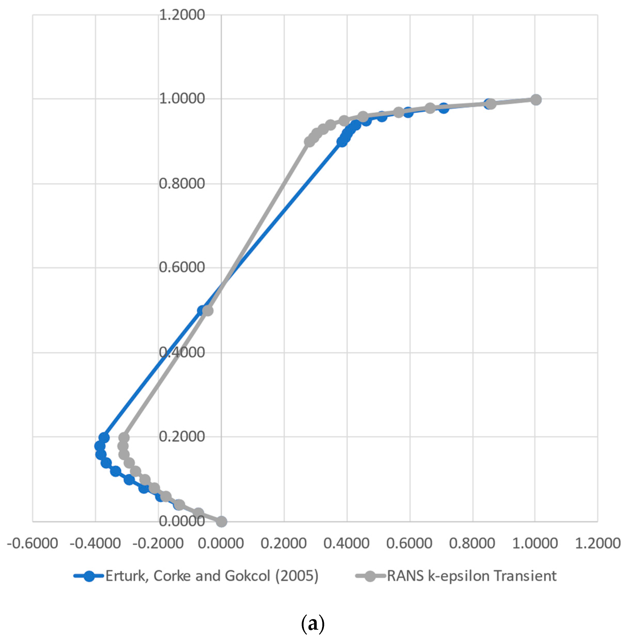
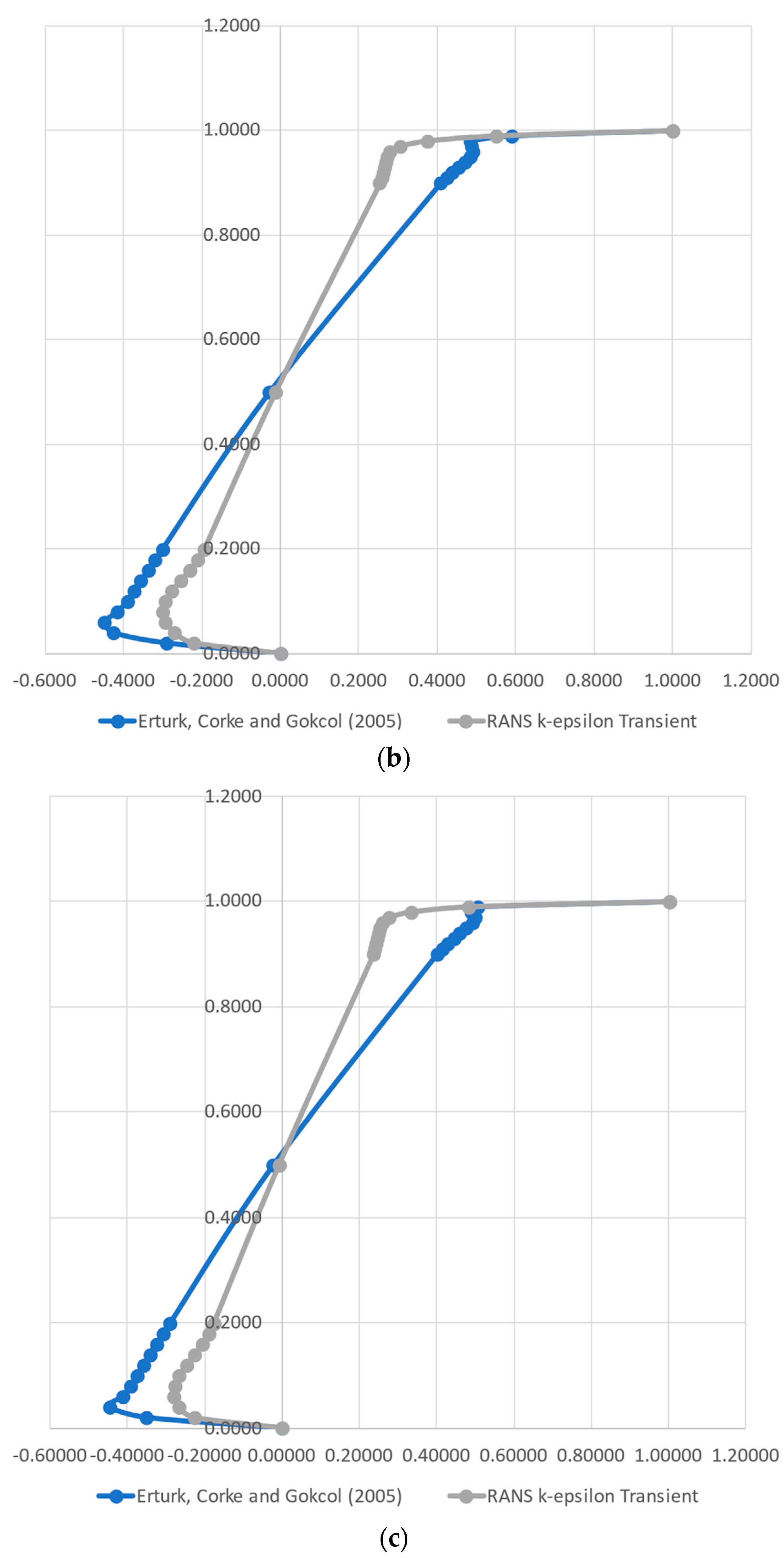
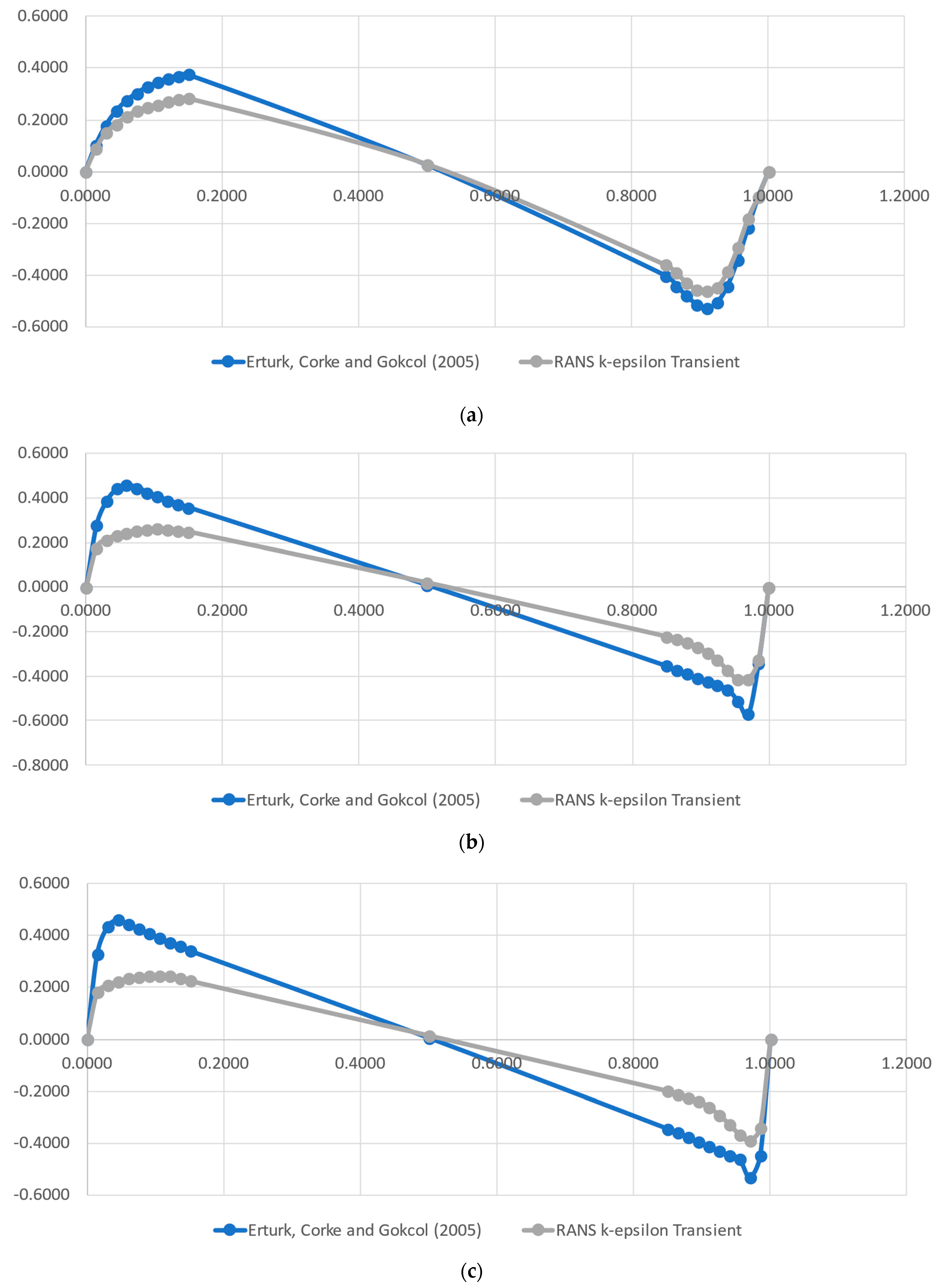
A complete Direct Numerical Simulation (DNS) flow solution was generated employing OpenFOAM. This approach required large time and computer resources, when compared with the simpler RANS k-ɛ turbulence model for a minimal gain on the proof of concept for our case. Therefore, we proceeded with the analysis, employing the classical RANS k-ɛ model for validation, which was carried out using the data from [
37], whose authors implemented a numerical method for 2D Steady Incompressible Navier–Stokes equations in streamfunction and vorticity formulations. For this task, the authors solved the lid-driven cavity flow to Reynolds numbers in the range of 1000–21,000. The authors provided the normal velocity components along a vertical and a horizontal line in the middle of the domain, i.e., the x component on the vertical line and the y component on the horizontal line. They used a high-order simulation to generate highly accurate data for the investigated Reynolds numbers. This approach permits taking values at critical points, which present highly variable shear stresses and vorticity.
2.2. Models’ Architecture Setup
To compare the capacity of the ML models to precisely predict the flow characteristics, three DL models were built and tested using the PyTorch library for the Python language. These were, namely, Convolutional Long Short-Term Memory (ConvLSTM), 2D CNN + LSTM and the Fourier Neural Operator (FNO).
For each one, several architecture configurations were tested, with the aim to identify the ones that provide the greatest balance between performance and computational load. The models were implemented in a standard form, already including the boundary conditions data in the input dataset. A set of configurable hyperparameters was proposed, and because exhaustively testing possible configurations would incur a prohibitive computational time, 10 random configurations were tested for up to 50 epochs instead. We could perceive that it was enough to achieve the best results for each base model. The best architectures were chosen to be more deeply trained, using up to 300 epochs. Further details about the tested architectures for each model are presented in the next subsections.
During all the steps of the work, the training parameters were fixed. We selected the cases of Re = 1000, 2000, 4000, 6000, 14,000, 16,000, 18,000 and 20,000 for the data for training and the Re = 10,000 case for testing, to develop the models’ architecture and compare their overall performance under the same conditions. The training and testing data included only the first 10 s of the simulation, as most flow dynamics were contained in this time frame. This simulation, with timesteps of 0.1 s, was divided into sequences of 3 inputs and 1 output, so our models were trained to forecast ti+3 given the input sequence {ti, ti+1, ti+2}.
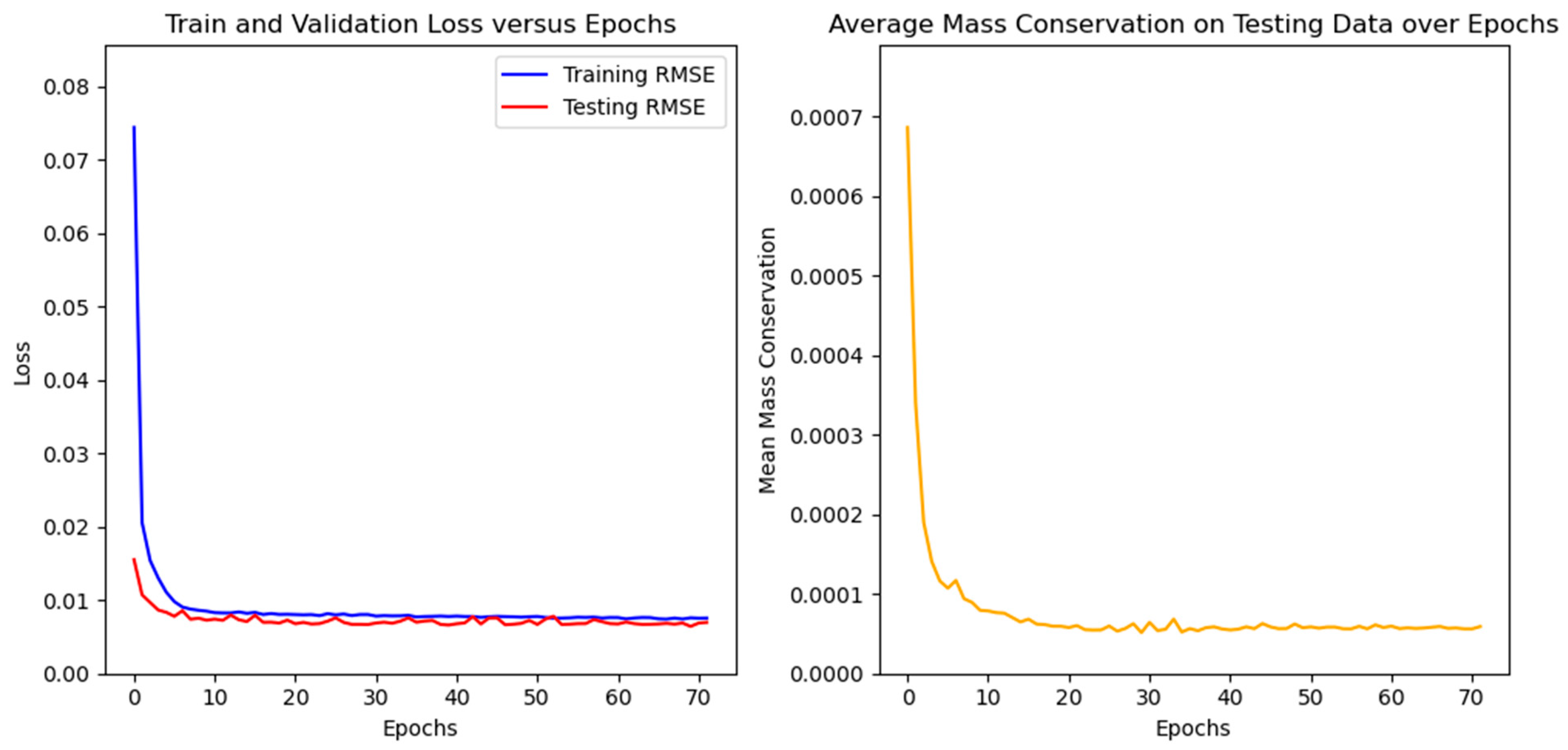
The learning rate was set to 1 × 10⁻³, and a scheduler was used to reduce its value by a factor of 2, whenever the validation loss stopped improving. The number of epochs could vary, because we used a “scheduler patience” of 10 epochs and implemented early stopping with a patience of 50 epochs. We used the overall Root-Mean-Square Error (RMSE), including the velocity components as well as the pressure, to assess the models’ performance on the training and testing sets, as well as to plot predictions to visualize the models’ forecasting accuracy. It is important to clarify that, even though the pressure field was also used to calculate the RMSE along with the x and y velocity fields, its value is always about 10 times smaller than theirs. In this sense, we opted to present the RMSE in units of m·s−1, which gives a physical meaning to the error without incurring any perceptible deviation.
2.2.1. ConvLSTM
A ConvLSTM is essentially an LSTM where the internal gates are modified to operate over two-dimensional data, which allows it to be used for spatial-temporal prediction. This is achieved by using convolution operations in the state-to-state and input-to-state transitions of the traditional LSTM gates [
38].
A multi ConvLSTM layer network was built and tested. The general structure was built by stacking multiple ConvLSTM cells in sequence, to test how the number of hidden dimensions, the kernel size and the number of layers affected performance.
2.2.2. Two-dimensional CNN + LSTM
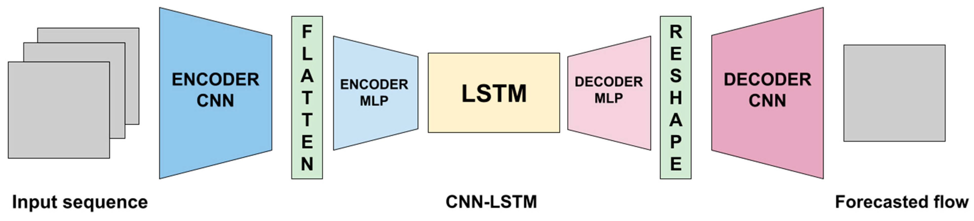
For this DNN paradigm, 2D CNN (convolution + max pooling) layers were used to create a deep autoencoder network, with an LSTM network added at the end of the network (
Figure 1). An additional linear layer was used to map the flattened output of our convolutional encoder to the latent dimension selected for use in the LSTM. In the same way, an additional linear layer was used to map the output of the LSTM back to the appropriate size such that the data could be reshaped back.
Like the other models, we randomly tested the optimal quantity of contiguous CNN layers, as well as the hidden channels and the dimension of the latent space of the DNN, i.e., how much information is retained and processed between the encoder and decoder MLPs (
Figure 1). Based on previous tests, only one LSTM layer was added. In [
39], the authors applied a similar procedure, successfully testing a similar DNN paradigm for solar irradiance modeling.
2.2.3. Fourier Neural Operator
The Fourier Neural Operator (FNO) has one important reported advantage over classical methods (all CFD as well as ML methods). The FNO models the solution operator, for not only one instance but also multiple instances at a time [
27]; this means that its tuning is not restricted to a specific solution case, being more generalizable than other ML approaches. In our work, we implemented this capability by training and testing the Physics-Informed Neural Network (PINN) for different Reynolds numbers.
The structure of the tested models was mounted by stacking contiguous FNO layers sequentially, up to 3. The current research evaluated the number of Fourier modes to keep (modes) in each layer (up to 16, in powers of 2), as well as the number of transforms to apply to these Fourier modes (width, up to 32, in powers of 2). It was expected that the FNO could capture the intrinsic PDE information, because its mapping occurs in the Fourier space (based on frequency modes), not Euclidean (based on spatial coordinates), as usual. This commonly may represent, or be near, the real solution of the PDE.
2.3. Application of Physical Information to the Models
After choosing the best architecture of each NN paradigm, we tested the effects of imposing physical constraints onto the models. This was performed via soft constraints [
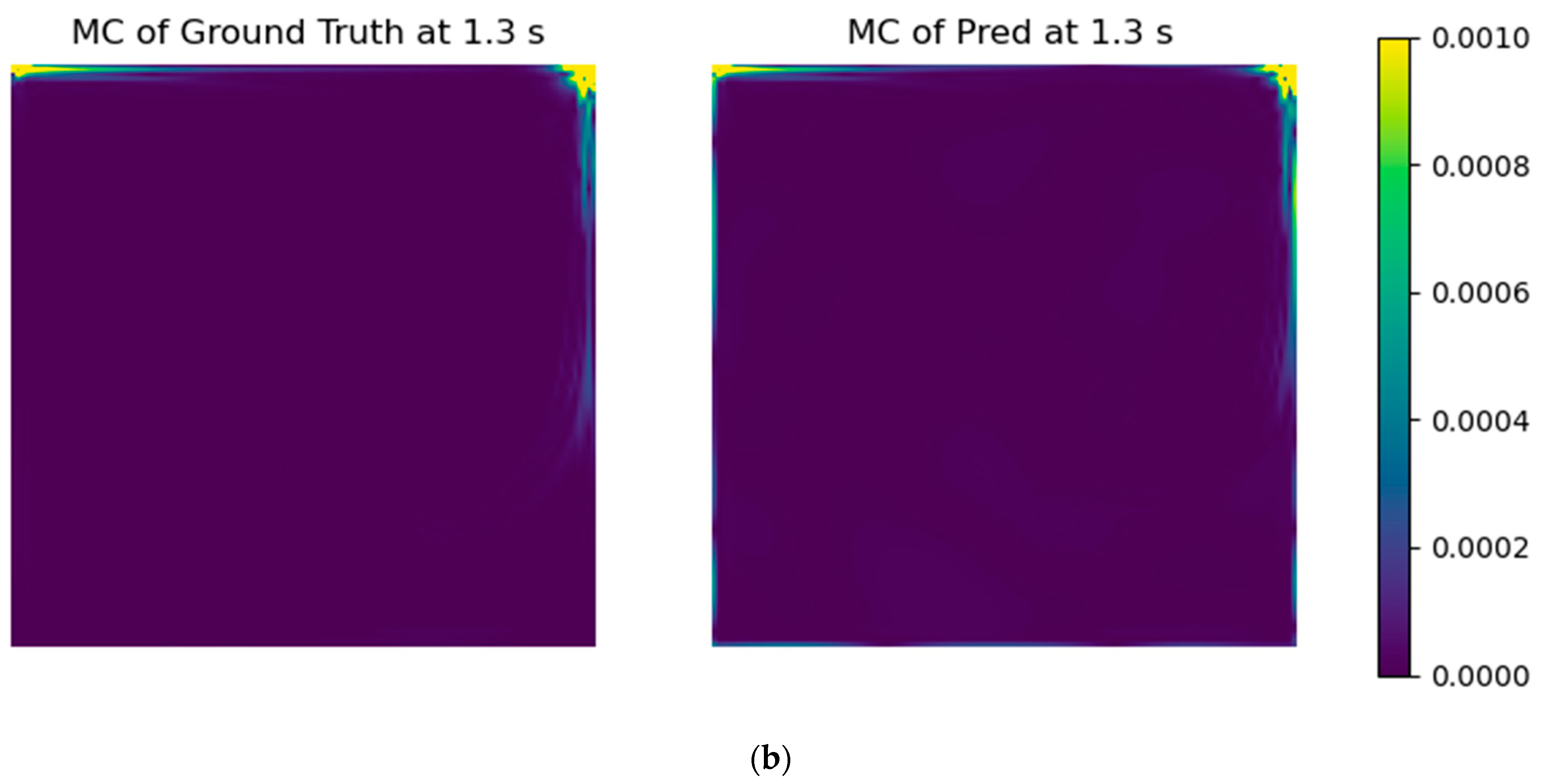
23], namely adding an error formula to drive the solution to mass conservation through the usual loss function. It was performed by calculating the mass flow imbalance (Equation (1)) for each grid cell and taking the arithmetic mean of their absolute values for all of the computational domain. It should be further noted that the values at the boundaries are already in the datasets, which also gives physics information to the models. The aim of the mass conservation error evaluation is to insert physical coherence into the models, improving interpretability and accuracy.
where the overall mass flux can be defined as
Because Cartesian coordinates are being used, it is straightforward to solve the above integral only using the velocity components and the side lengths of each cell.
The governing equations, in a non-dimensional form, for the 2D lid-driven problem are [
31,
34]
where
are the velocities for the 2D case, and
and t are pressure and time, respectively.
represents the Reynolds number, defined as a ratio between the product of velocity and lid length over the kinematic viscosity. For the boundary conditions, the velocities were set to zero over the lateral walls and to finite non-zero over the upper wall. For the domain walls, both epsilon and P were set as having zero gradient. Last, k was set to zero over the domain’s walls.
At this stage, several weights were tested for the calculated errors of mass conservation, trying to optimize the PINNs results. The tested values were 0.0, 0.1, 1.0, 2.0 and 5.0.
2.4. Number of Timesteps (Moving Time Window)
Aiming to quantify generalizability to assess how performance degrades with the degree of extrapolation, under unseen initial conditions [
23], we tested the influence of the training time window size on the models’ performance, following a similar approach that is usually performed in CFD. Once the improved PINNs were developed at this stage, we took the best two models, namely ConvLSTM and FNO, to assess their performance under several time window configurations. This was performed first by forecasting 10 timesteps in advance, each one separately, i.e., we ran the model to forecast the next timestep, and then we use this forecasted field to predict the next one, and so on. In this stage, we tested input timestep windows with sizes of 1, 3, 6, 10 and 15, aiming to mimic different orders of time discretization, a standard approach in CFD. It is worth mentioning that the implementation of high-order time discretization (e.g., from 3 and above) is usually a complex task in CFD, whereas in DNN, it is almost straightforward, being just a matter of training set selection.
After this stage, we tested another approach, where we took the best input time window size and forecasted different size outputs, this time being the prediction directly obtained by the models in a single step. The tested output sizes were 1, 3 and 10, and they were applied to directly predict 10 timesteps in advance. It is worth mentioning that, based on the time resolution (0.1 s) and the lid velocity for the testing set (1.0 m·s−1), 10 timesteps correspond to a complete pass of the lid by the solution domain.
4. Discussion
Research efforts have been carried out in order to model turbulent flows. The approach of using classical problems that, in a simple way, manage to represent complex phenomena is often used [
40]. In this context, cavity flow is commonly applied under various conditions and for different purposes. In [
41], the authors proposed the combined solution of CFD with Back Propagation for modeling a cavity with a backward-facing step, and as can be seen in our work, the technique is promising and deserves investigation.
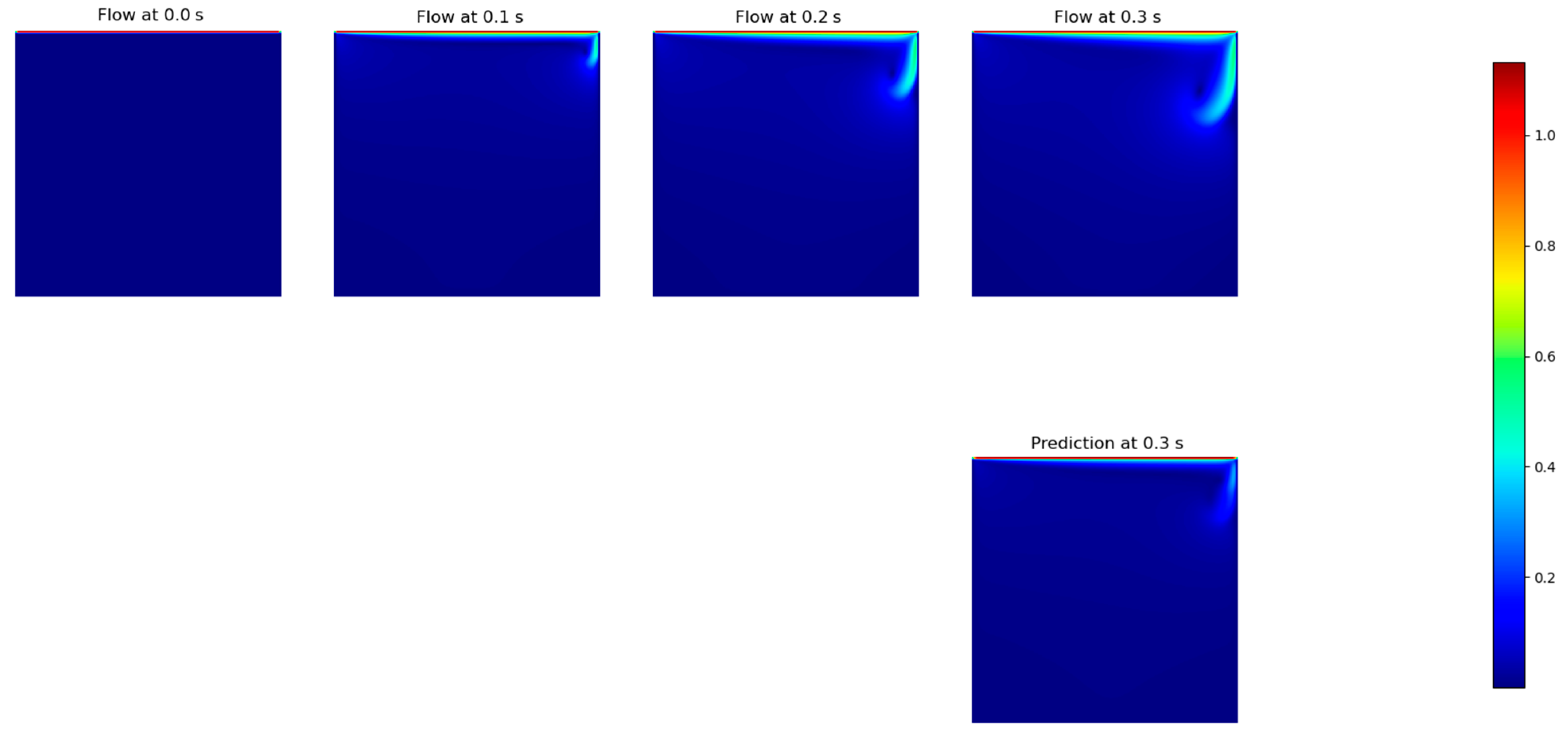
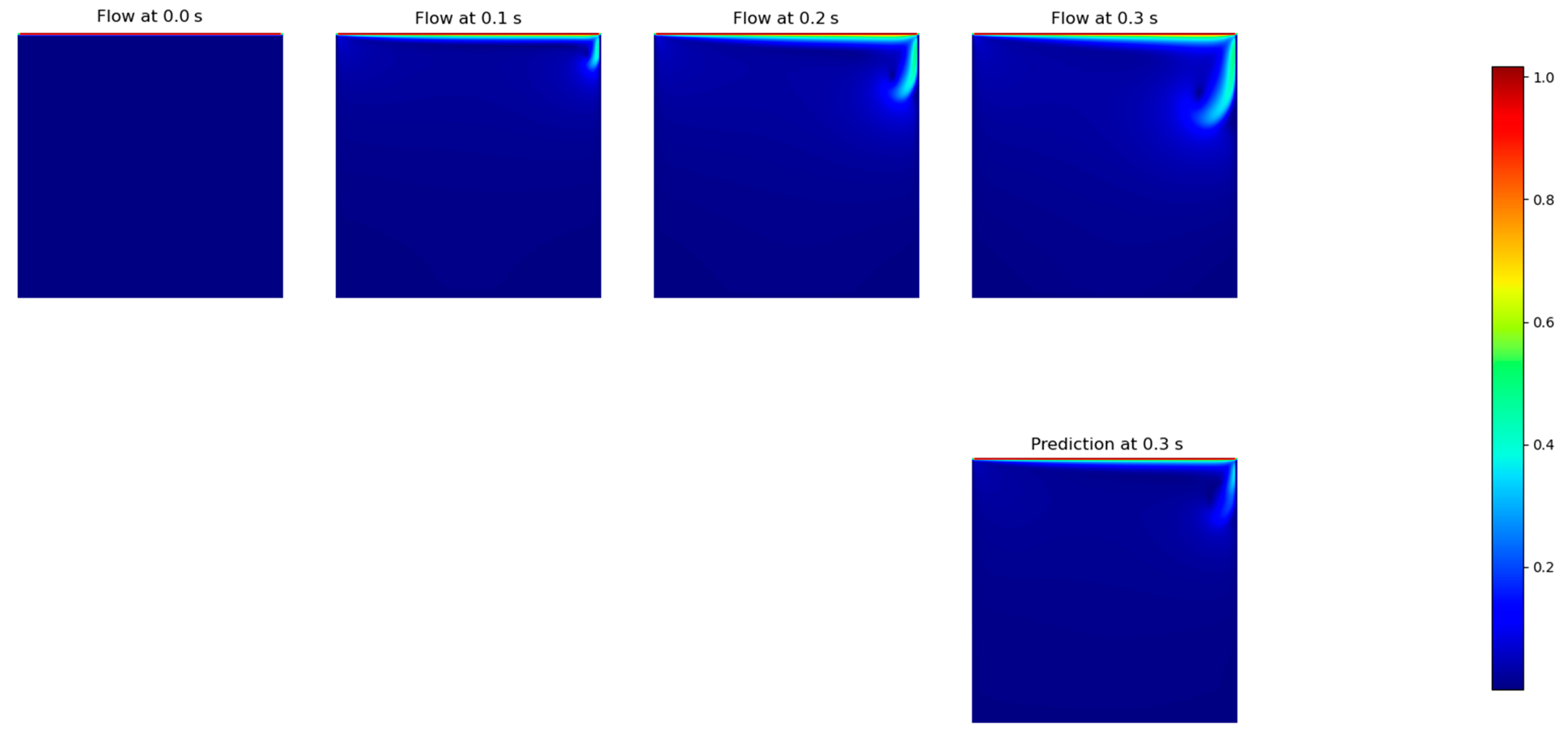
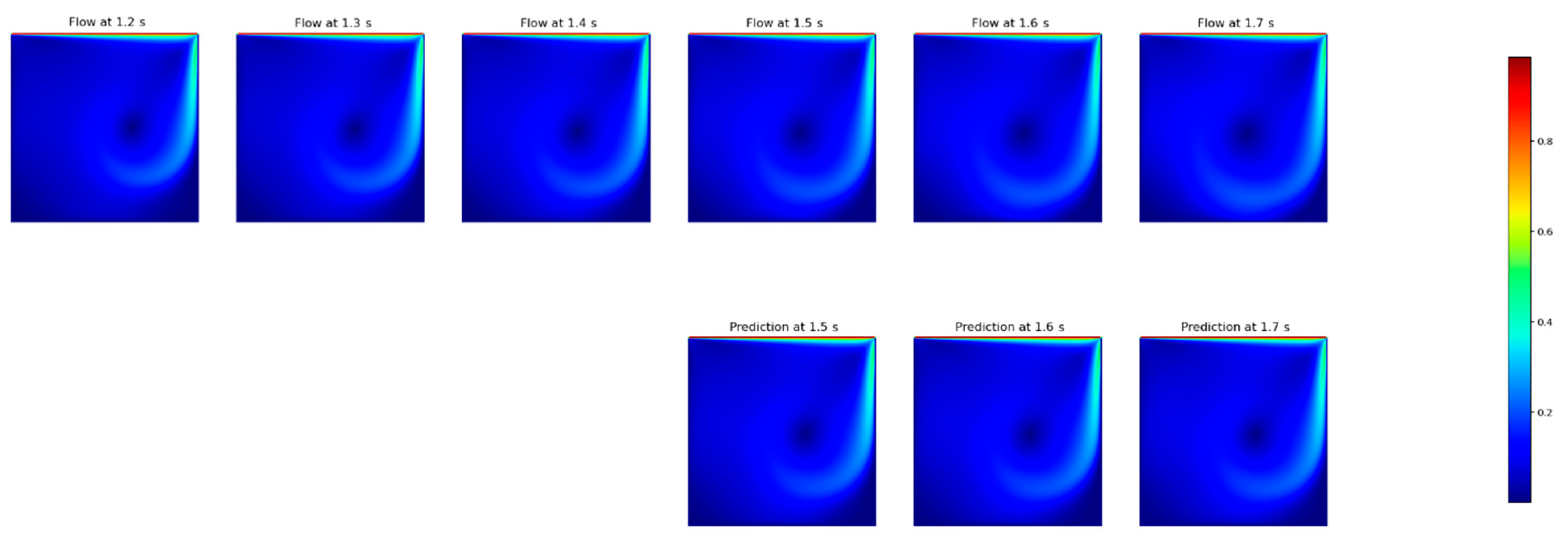
In the present work, we focused on comparing classic DNN architectures with the recent FNO approach. In general, the DNN approach tends to dissipate flow energy, which can be evidenced by a reduction in eddy viscosity [
42], as well as a reduction in vorticity, which can be shown, as we present here, in the difficulty of the models to maintain the rotation of the flow. In this regard, we were able to indicate that the investigated FNO-based DNN architecture did not show improvements in the flow prediction capability for timesteps greater than three, as presented in
Table 6.
Regarding the performance of the developed architecture, it managed to reach levels equivalent or even superior to those presented in the literature and required reduced training time due to its simpler implementation. Our MSE of 4.13 × 10
−5 is in the same order of magnitude as that of [
43], where the authors obtained their values for Burgers’ equation, the Sine-Gordon equation, the Allen–Cahn equation and Kovasznay flow. For the cavity, our results are much better than the best result reported by them, MSE = 8.9456 × 10
−2.
It is common in works involving DNNs to use different performance evaluation metrics, which makes direct comparison between approaches difficult. In [
28], the authors used the L2 relative error to evaluate several DNN architectures, specifically based on DeepONet and FNO. Despite this, as we also point out here, the approaches based on the FNO stood out for their superior performance.
Given the above, the feasibility of the technique is strongly indicated, as also found in the recent literature [
14], where there was no quantitative presentation of the error, but which qualitatively showed the robustness of the Physics-Informed Neural Network solution. This viability is also already shown with realistic problems, such as the cavity flow studied here. The authors of [
24] presented MAE in the order of 1 × 10
−3, which is at the same level of our reached RMSE. It is noteworthy that the RMSE metric always tends to be greater than the MAE for the same problem, which indicates that the FNO is fully qualified for the development of research of Physics-Informed Neural Networks.
5. Conclusions
This paper presents a novel approach to solve the Navier–Stokes equations using Physics-Informed Neural Networks. Three DNN paradigms (Fourier Neural Network, Convolutional LSTM and CNN-LSTM) were implemented and tested against the CFD solution of the cavity lid-driven flow problem. We used several Reynolds numbers to test and forecast the Re = 10,000 case, aiming to benchmark the Fourier Neural Network (FNO). The advantage of this new class of DNN architecture is the mapping of fields between different spaces (not necessarily Euclidean), which allows the learning of the parametric dependence of the solutions directly to an entire family of PDEs. From the results, the following conclusions can be highlighted:
A RANS k-ε CFD solution was performed to generate data (training and testing) to be fed to the models. A comparison with the results found in the literature was able to attest the data quality. The evaluation of the k-ε turbulence model against a full Direct Numerical Simulation indicated that the simpler CFD model, for this simple case, accurately represented the turbulence phenomena.
After the tests for the models’ architectures setup, the FNO and ConvLSTM paradigms performed better, with a consistent small advantage of FNO.
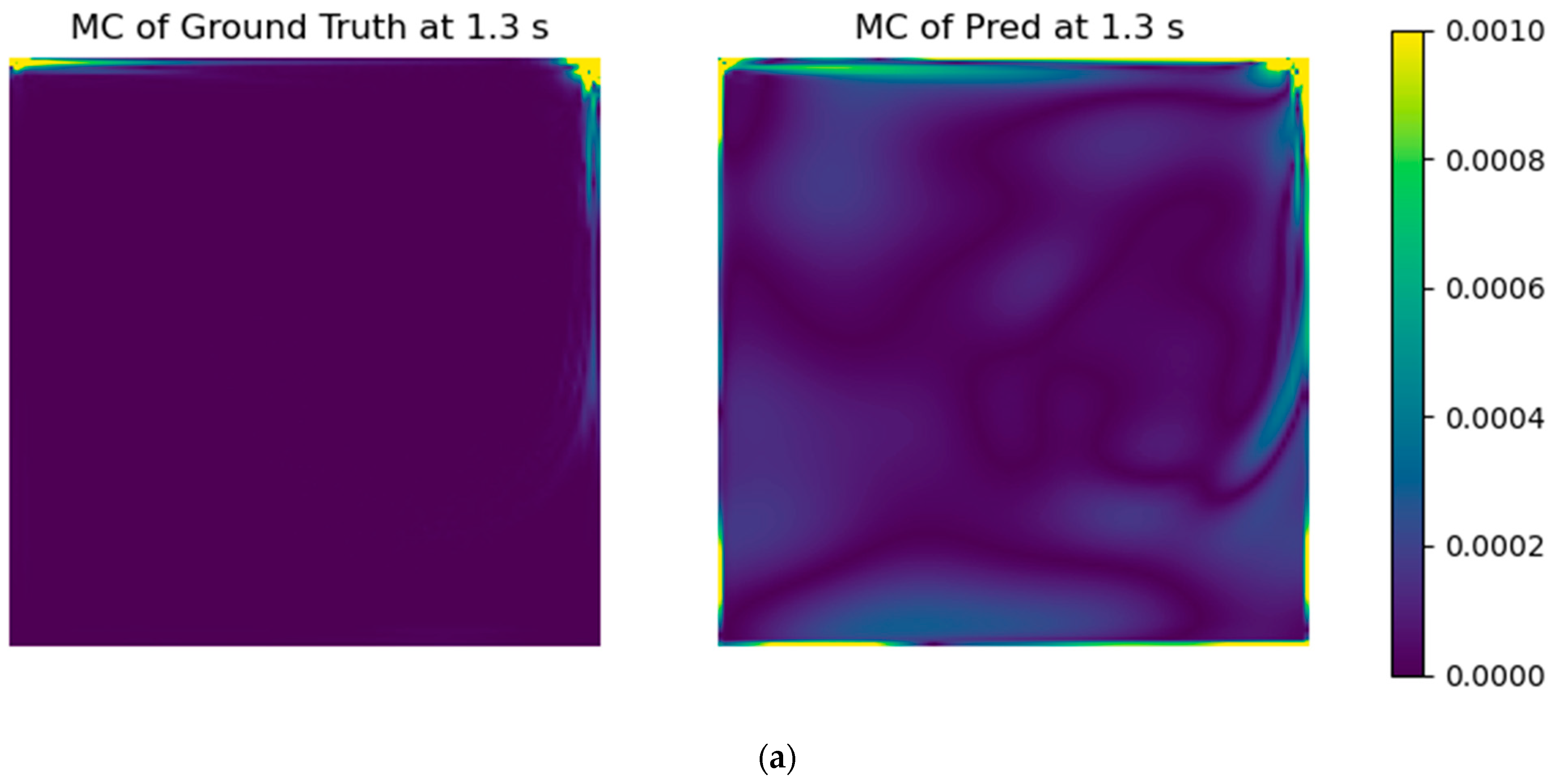
With the selected models’ architectures, a custom error parcel regarding the mass conservation error was added to the training step, using several weight values. Even though the RMSE of the test case did not improve, the resultant fields presented a notable improvement in physical coherence.
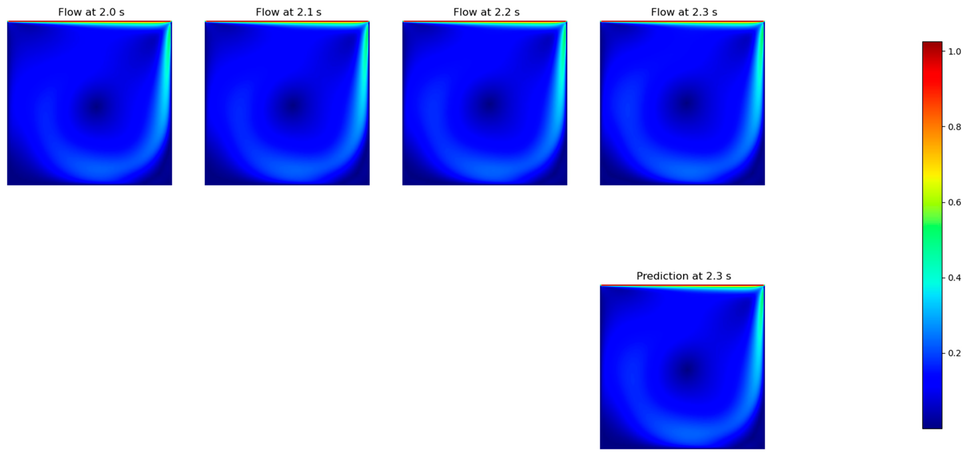
The FNO paradigm was finally assessed to predict the solutions of the flow under several input/output situations, giving a testing RMSE of 0.008792 m/s for the best configuration (three timesteps for the input and three timesteps for the output), which was at least two orders of magnitude of the reference lid velocity (1.0 m/s).
For the tested case, the FNO was able to consistently perform better than the other models, which qualifies it as an option to further develop DNN solutions of partial differential equations. Although presenting good performance, the FNO has some limitations, as presented by Lu et al. [
28], and DeepONet is an option to address such hindrances. For further work, implementation of the momentum conservation equation to the model could be performed to assess its contribution over the model’s results, as well the effect of different image resolutions in the final model’s prediction. Moreover, a deeper understanding of FNO limitations can be assessed by testing other problem configurations and the effect of turbulence levels, not only for RANS models, but also for Large-eddy Simulations or Direct Numerical Simulation (DNS) results. For instance, other flow geometries can be tested, which would produce more transient solutions of the PDEs, such as a bluff body or wake flows. Moreover, greater Reynolds numbers can be considered, which may be indicative of environmental flows.


 ,
, 


