Dimension Reduction and Redundancy Removal through Successive Schmidt Decompositions

Abstract

Quantum computers are believed to have the ability to process huge data sizes, which can be seen in machine learning applications. In these applications, the data, in general, are classical. Therefore, to process them on a quantum computer, there is a need for efficient methods that can be used to map classical data on quantum states in a concise manner. On the other hand, to verify the results of quantum computers and study quantum algorithms, we need to be able to approximate quantum operations into forms that are easier to simulate on classical computers with some errors. Motivated by these needs, in this paper, we study the approximation of matrices and vectors by using their tensor products obtained through successive Schmidt decompositions. We show that data with distributions such as uniform, Poisson, exponential, or similar to these distributions can be approximated by using only a few terms, which can be easily mapped onto quantum circuits. The examples include random data with different distributions, the Gram matrices of iris flower, handwritten digits, 20newsgroup, and labeled faces in the wild. Similarly, some quantum operations, such as quantum Fourier transform and variational quantum circuits with a small depth, may also be approximated with a few terms that are easier to simulate on classical computers. Furthermore, we show how the method can be used to simplify quantum Hamiltonians: In particular, we show the application to randomly generated transverse field Ising model Hamiltonians. The reduced Hamiltonians can be mapped into quantum circuits easily and, therefore, can be simulated more efficiently.

1. Introduction

Quantum computers are considered to be theoretically more efficient than classical computers: ${\displaystyle BPP\subseteq BQP}$, which are the complexity classes for the problems that are solvable with a bounded error, respectively, on a probabilistic machine and a quantum computer. For instance, in the search for an item among unstructured ${\displaystyle N}$ items, quantum computers can go beyond the theoretically proven classical lower bound of ${\displaystyle O\left(N\right)}$ and find an item in ${\displaystyle O\left(\sqrt{N}\right)}$ steps [1]. In addition, although currently there is not a known classical poly-logarithmic algorithm for integer factorization or similar problems, these problems can be solved on quantum computers in poly-logarithmic time by using Shor’s factoring algorithm [2] (see Ref. [3] for quantum algorithms in general). However, it is still unknown if ${\displaystyle BPP=BQP}$ or if the separation is polynomial or exponential (see, e.g., [4]). Note that although Shor’s algorithm indicates an exponential speed up over the currently known classical algorithms, since the integer factorization is not a proven NP-complete or NP-hard problem, this does not mean one can solve general NP-complete problems in polynomial time on quantum computers. However, one can construct some instances similar to (or can be mapped into) the integer factorization and then solve them with Shor’s algorithm [5], even though we still do not know if those instances naturally exist in any practical problem [6].

Any quantum computation can be represented by an ${\displaystyle N\times N}$ matrix acting on ${\displaystyle n=log\left(N\right)}$ number of qubits. According to Solovay–Kitaev theorem [7,8], any quantum operation can be approximated by using single and two-qubit quantum gates where the approximation error is determined by the number of gates. In general, an ${\displaystyle N\times N}$ matrix requires ${\displaystyle O\left(N^2\right)}$ numbers of single and CNOT gates (or any two-qubit entangling gate) for an exact representation since the matrix may have up to ${\displaystyle N^2}$ number of independent coefficients [9]. From this, one may argue that simulating a given general matrix computation on quantum computers in ${\displaystyle O\left(poly\right(n\left)\right)}$ with a certain accuracy may not be possible. Therefore, we assume the complexity classes ${\displaystyle P}$ and ${\displaystyle NP}$ are not equal; quantum computers, in general, cannot solve NP-complete problems with the ${\displaystyle n}$ number of parameters in ${\displaystyle O\left(poly\right(n\left)\right)}$ because the solution of these problems can be mapped to a simulation in a matrix-vector transform with sizes ${\displaystyle O\left(N^2\right)}$ and ${\displaystyle O\left(N\right)}$ [10,11]. This means that although we know that some problems can be solved more efficiently, it is still not fully known whether a meaningful quantum computation with ${\displaystyle poly\left(n\right)}$ quantum operations are beyond the capacities of classical computers: i.e., under certain conditions, such as a special memory structure; if the result of the computation can be obtained from the given input in ${\displaystyle O\left(poly\right(n\left)\right)}$ by a classical computer (by using generally randomized algorithms).

Machine-learning tasks on quantum computers have started with various types of proposals for quantum neural networks to either speed up the learning task or provide a better neural network model, e.g., quantum mechanics modeling human-neuron systems [12], quantum dots [13,14], or general quantum computational tools, are being used to describe classical neural networks [15]. After Lloyd’s seminal paper [16] that provided a poly-logarithmic algorithm for principal component analysis of data stored in quantum ram (the data are given as quantum states), the research on quantum machine learning and quantum big data analysis gained a lot of attention and momentum (see [17,18] for a review of the area and [19] for an introduction with a comparative analysis to classical machine learning). The quantum principal component analysis leads most researchers to believe that quantum computers may provide exponential speed up for data analysis tasks. However, it is shown that by using a classical data structure similar to the assumptions made on the quantum algorithm, one can also perform the same analysis task on classical computers exponentially faster [20]. Although with the currently known quantum algorithms, exponential speed up is not known, some quantum versions of the data analysis algorithms are still faster in terms of computation complexity [20]. In addition, quantum computers are expected to be able to handle more data. Therefore, they would be more powerful in terms of computational space and capacity. Some of the quantum versions of the classical algorithms are also shown to be more accurate for the same machine-learning problems [21,22].

1.1. The Motivation

1.1.1. Mapping Data into Quantum States to Run on Quantum Computers

Using parameterized quantum circuits (so-called variational quantum circuits, VQC), one can generate a matrix ${\displaystyle U\left(\mathit{\theta }\right)}$ whose transformation depends on the parameters given by the vector ${\displaystyle \mathit{\theta }}$: i.e., the parameters define the specifics for the quantum gates, such as the angle values. In general, because of the training and computational difficulties, the design structure of ${\displaystyle U\left(\mathit{\theta }\right)}$ is fixed by using quantum gates, which guarantees the entanglement of the qubits and certain computational prowess.

In many recent quantum machine learning models, various types of variational quantum circuits are used as a replacement to a model of a neural network. Given different inputs as the initial state of the quantum circuit, training in these models is generally performed by classically optimizing the parameters of the circuits. In other words, the learning task aims to find a circuit ${\displaystyle U\left(\mathit{\theta }\right)}$ so that for an input ${\displaystyle \left|\psi \right.〉}$ representing a data vector, ${\displaystyle U\left(\mathit{\theta }\right)\left|\psi \right.〉}$ outputs a state from which the expected result can be obtained through quantum measurements with high probability.

In this learning model, one of the fundamental tasks is to find a way to map a data vector ${\displaystyle \mathit{x}}$ into a quantum state ${\displaystyle \left|\psi \right.〉}$ without losing any information. This can be performed in two different ways [17,18,23,24]: (i) as performed in neural networks, we use one qubit for each feature ${\displaystyle x_i}$. Because of the similarities to classical neural networks, this mapping provides a natural way to perform quantum machine learning with variational quantum circuits. However, the difficulty is that the required number of qubits may be very high and is very likely beyond the capabilities of current (may also be near future) quantum computers. (ii) We can consider ${\displaystyle \left|\psi \right.〉=\mathit{x}/\parallel \mathit{x}\parallel }$. Although the learning task may become more difficult, the number of qubits becomes exponentially small in comparison to the dimension of the data vector; we will use ${\displaystyle N=2^n}$. However, generating a general ${\displaystyle \mathit{x}}$ requires ${\displaystyle O\left(N\right)}$ quantum gates. This complicates the simplicity of the variational quantum circuits and impedes the applications to the problems with high dimensional data vectors. As a result, as in the classical data analysis, for quantum computers, we need to find methods similar to the singular value decomposition [25] to reduce the dimensions of data sets in a way so that we can reduce the required number of qubits and the number of quantum gates.

1.1.2. Classical Simulation of Quantum Circuits and Designing More Efficient Quantum Circuits

Simulating quantum operations is difficult when the qubits are entangled. It is known that quantum operations can be efficiently simulated by taking advantage of their mathematical structures, which are generally studied by using tensor networks [26,27]. Tensor networks are used to simulate quantum systems more efficiently and approximate them with certain accuracy (e.g., [28,29]).It is also well known that the bipartite entanglement can be understood by using the Schmidt decomposition of the bipartite system [30,31].

Recently, it has been shown that the coefficients in the Schmidt decomposition of quantum Fourier transform exponentially decay; thus, the quantum Fourier transform may be efficiently simulated on classical computers and also may be more efficient than the classical algorithms for the discrete Fourier transform [22]. It is also shown that the entanglement can be classically forged through the Schmidt decomposition to combine the results of two separate quantum operations on classical computers [32].

Motivated by the above two points, in this paper, we study the approximation of matrices and vectors by using their tensor products obtained through successive Schmidt decompositions. We show that some data distributions can be approximated by using a few terms that can be easily mapped into quantum circuits. Similarly, some quantum operations may also be approximated with high accuracy that is easier to simulate on classical computers.

In the following, we first explain Schmidt decomposition and draw an equivalent recursion tree that can be used to understand the decomposition. Then, we describe how this tree can be used to eliminate the terms with lower coefficients and generate approximated quantum operators. In Section 3, we show the applications of the method to random data vectors, Gram matrices, and general symmetric matrices on example machine learning datasets: Iris flower, handwritten digits, 20newsgroup, and labeled faces in the wild. Then, after discussing how it can be used in solving systems of linear equations, we show the approximation of the quantum Fourier transform in Section 3.3. Then, we study the dataset with a circular type distribution in Section 3.4 and variational quantum circuits with different depths in Section 3.5. In our final example, in Section 3.6, we show how the method can be applied as an approximation tool to reduce the terms in a transverse field Ising model of quantum Hamiltonians. After showing how classical and quantum computation can be performed with the approximated forms, we conclude the paper.

2. The Schmidt Decomposition and Its Recursion Tree Structure

In the following notations, we use bold-face or the Dirac bra-ket notations for the vectors: ${\displaystyle \left|x\right.〉}$ and ${\displaystyle \mathit{x}}$ are equivalent, but the former represents a quantum state that is generally normalized. The matrices are written in capital letters.

2.1. Singular Value Decomposition (SVD) [25]

For any ${\displaystyle M\times N}$ matrix, ${\displaystyle A}$, there exists a factorization of the form:

$$A=U\mathsf{\Sigma }{V}^{*}=\sum _i^r{\sigma }_i{\mathit{u}}_{\mathit{i}}{\mathit{v}}_{\mathit{i}}^{*},$$

(1)

where ${\displaystyle U}$ and ${\displaystyle V}$ are ${\displaystyle M\times M}$ and ${\displaystyle N\times N}$ unitary matrices and ${\displaystyle \mathsf{\Sigma }}$ is an ${\displaystyle M\times N}$ rectangular diagonal matrix with positive diagonal entries ${\displaystyle {\sigma }_1\ge {\sigma }_2\cdots \ge 0}$, known as singular values. ${\displaystyle r}$, the number of non-zero singular values, defines the rank of the matrix and is the min of ${\displaystyle M}$ and ${\displaystyle N}$.

Let ${\displaystyle vec\left(A\right)}$ be the vectorized form of matrix ${\displaystyle A}$. The SVD can be used to write this vector into a sum of weight-ordered separable components:

$$vec\left(A\right)=\sum _i{\sigma }_i{\mathit{u}}_{\mathit{i}}\otimes {\mathit{v}}_{\mathit{i}}.$$

(2)

Note that SVD provides the closest low-rank approximations in ${\displaystyle l^2}$-norm to the matrix. For instance, a rank ${\displaystyle r_1\le r}$ approximation can be obtained by:

$$A=\sum _i^{r_1}{\sigma }_i{\mathit{u}}_{\mathit{i}}{\mathit{v}}_{\mathit{i}}^{*}.$$

(3)

2.2. Schmidt Decomposition [30,31]

Let ${\displaystyle \left|\psi \right.〉}$ represent a ${\displaystyle n}$-qubit system (${\displaystyle N=2^n}$), where qubits are ordered as ${\displaystyle q_0{q}_1\cdots q_{n-1}}$. Using the Schmidt coefficients between the first qubit ${\displaystyle q_0}$ and the rest of the system, i.e., ${\displaystyle q_0\text{—}(q_1\cdots q_{n-1})}$, we can represent the state in the following form:

$$\left|\psi \right.〉={\sigma }_1\left|u_1\right.〉\otimes \left|v_1\right.〉+{\sigma }_2\left|u_2\right.〉\otimes \left|v_2\right.〉.$$

(4)

In the above, while ${\displaystyle {\sigma }_1^2+{\sigma }_2^2=1}$, ${\displaystyle 〈u_1|u_2〉=1}$ and ${\displaystyle 〈v_1|v_2〉=1}$. The Schmidt decomposition of a vector can be found by converting the vector into a ${\displaystyle 2\times 2^{n-1}}$ matrix and using the SVD described above. In that case, ${\displaystyle {\sigma }_1}$ and ${\displaystyle {\sigma }_2}$ are the singular values and ${\displaystyle \left|u_i\right.〉}$ and ${\displaystyle \left|v_i\right.〉}$s are the singular vectors.

Here, we can keep recursively taking the Schmidt decomposition of the larger vectors, i.e., ${\displaystyle \left|v_i\right.〉}$s, and obtain the following:

$$\begin{array}{cc}\hfill & \left|v_1\right.〉={\sigma }_3\left|u_3\right.〉\otimes \left|v_3\right.〉+{\sigma }_4\left|u_4\right.〉\otimes \left|v_4\right.〉,\mathrm{and}\hfill \\ \hfill & \left|v_2\right.〉={\sigma }_5\left|u_5\right.〉\otimes \left|v_5\right.〉+{\sigma }_6\left|u_6\right.〉\otimes \left|v_6\right.〉.\hfill \end{array}$$

(5)

Note that the size of any ${\displaystyle \left|u_i\right.〉}$ is still two by two. Once the size of ${\displaystyle \left|v_i\right.〉}$ also goes down to two, we stop the recursion. In the final analysis, we can write ${\displaystyle \left|\psi \right.〉}$ in the following decomposed form:

$$\begin{array}{cc}\hfill \left|\psi \right.〉=& {\sigma }_1\left|u_1\right.〉\otimes {\sigma }_3\left|u_3\right.〉\otimes {\sigma }_7\left|u_7\right.〉\otimes \cdots \hfill \\ \hfill & +{\sigma }_1\left|u_1\right.〉\otimes {\sigma }_3\left|u_3\right.〉\otimes {\sigma }_8\left|u_8\right.〉\otimes \cdots \hfill \\ \hfill & +\hfill \\ \hfill & ⋮\hfill \\ \hfill & +{\sigma }_2\left|u_2\right.〉\otimes {\sigma }_6\left|u_6\right.〉\otimes {\sigma }_{14}\left|u_{14}\right.〉\cdots \hfill \\ \hfill & +\cdots =\sum _i\left|{\psi }_i\right.〉,\hfill \end{array}$$

(6)

where ${\displaystyle \left|{\psi }_i\right.〉}$ represents a term in the summation, and the number of terms is exponential in the number of qubits. Figure 1 shows the recursion tree for the above equation. In the figure, each path from the root node to a leaf node represents a summation term in the equation. If any of the coefficients, ${\displaystyle {\sigma }_i}$, is zero in this path, then the equivalent term in the summation is zero as well. Therefore, the number of non-zero terms is equal to the number of paths with non-zero coefficients.

2.3. Quantum Operations

The same recursion tree can also be generated for the operators. In that case, we use the following steps:

• Let ${\displaystyle A}$ be an ${\displaystyle N\times N}$ matrix. First, we vectorize matrix ${\displaystyle A}$ (column- or row-based vectorization can be used. In this paper, we will assume row-based vectorization.):

  $$\left|\psi \right.〉=vec\left(A\right).$$

  (7)
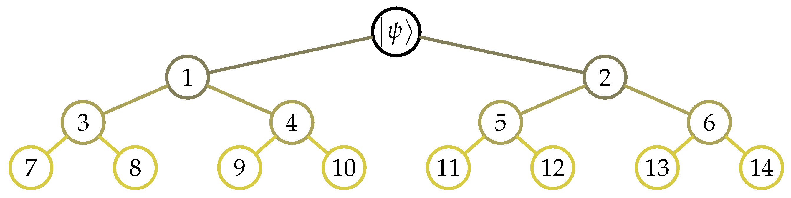
• Then we draw the recursion tree as in Figure 1.
• Since each path from the root to a leaf node is a ${\displaystyle N^2}$ by 1 vector, we can convert these terms back to ${\displaystyle N}$ by ${\displaystyle N}$ matrices. In that case, we can write ${\displaystyle A}$ as in the form:

  $$A=\sum _{i\in \{0,\cdots ,N^2/2\}|A_i\ne 0}{A}_i.$$

  (8)
• Note that the number of paths is equal to the number of leaf nodes, which is ${\displaystyle 2^n/2}$ for a vector of dimension ${\displaystyle 2^n}$.
• To convert a tensor decomposition of a vector into an operator in tensor form, let us consider the following example term:

  $$\left|{\psi }_j\right.〉=\left|p_1\right.〉\otimes \left|p_k\right.〉\otimes \left|q_1\right.〉\otimes \cdots \otimes \left|q_k\right.〉.$$

  (9)
  Assuming ${\displaystyle \left|p_i\right.〉}$ and ${\displaystyle \left|q_i\right.〉}$s are column vectors of dimension 2; from the definitions in Equations (1) and (2), we can convert this term into an operator ${\displaystyle A_j}$ as follows:

  $$A_j=\left|p_1\right.〉\left.〈q_1\right|\otimes \left|p_2\right.〉\left.〈q_2\right|\otimes \cdots \otimes \left|p_k\right.〉\left.〈q_k\right|=\underset{i=1}{\overset{k}{⨂}}\left|p_i\right.〉\left.〈q_i\right|.$$

  (10)
  Here, each ${\displaystyle \left|p_i\right.〉}$${\displaystyle \left.〈q_i\right|}$ is a 2 by 2 matrix and is not unitary. However, they can be written as a sum of two unitary matrices.

3. Approximation by Removing the Number of Paths with Smaller Coefficients

Choosing a threshold probability in the tree, we can approximate any operator or vector by eliminating the paths with coefficients lower than the threshold probability. To determine the approximation error between the normalized quantum state ${\displaystyle \left|\psi \right.〉}$ and the approximation ${\displaystyle \left|\varphi \right.〉}$ (not-normalized), we shall use the norm of the difference:

$$ϵ={∥\left|\psi \right.〉-\left|\varphi \right.〉∥}_2.$$

(11)

Note that this is equivalent to the sum of squared errors. One can also consider the mean squared error: ${\displaystyle {ϵ}^2/2^n}$, which is much smaller. In the following subsections, we show approximations of different cases and their approximation errors.

3.1. Approximation of Gram Matrix

Gram matrix [25] is frequently used in machine learning and other areas [33,34,35]. For a given data matrix ${\displaystyle X}$ (the column vectors represent the data), it is defined by the following product:

$$G=X^{T}X.$$

(12)

Matrix ${\displaystyle G}$ is positive semi-definite, and its rank depends on the number of independent data vectors in ${\displaystyle X}$. In the simulations, we have used the normalized ${\displaystyle vec\left(G\right)}$ produced from the default random number generator used in the Python-numpy package. The following Python code is used to generate data with different distributions. (The simulation code can be found on https://github.com/adaskin/app_with_schmidt.git, (accessed on 27 February 2023)):

import numpy as np
n = 8
N = 2**n
dist = "normal"
rng = np.random.default_rng()
if dist == "normal":
    X = rng.normal(size = (N,N))
elif dist == "uniform":
    X = rng.uniform(size = (N,N))
elif dist == "exponential":
    X = rng.exponential(size = (N,N))
elif dist == "poisson":
    X = rng.poisson(size = (N,N))
		

Using different distributions with default parameters, an example of the output, which shows the histogram of the probabilities of the paths, is presented in Figure 2 (Most output generates a similar result. Therefore, we only show one instance for each to explain the behavior in each distribution). As seen in the figure, in the cases of the exponential, Poisson, and uniform distributions, matrix ${\displaystyle G}$ can be approximated with high accuracy by using only one term. This is because the Schmidt decomposition is related to the eigenvalues of the data matrix, and the variance of the eigenvalues in these cases is large: i.e., there is one dominant eigenvalue. When the distribution is normal, although there is a clear cut-off point, the approximation accuracy is less than the others.

Here note that one can also use the same technique to directly approximate ${\displaystyle X}$. Figure 3 shows the direct approximations for instances of ${\displaystyle \left|\psi \right.〉=vec\left(X\right)}$ generated randomly from different distributions. As can be seen from the figure, although a cut-off point still exists in all except the normal distribution, the accuracy is much lower. We also note that in the normal distribution, since the data depends on most of the paths, the probabilities are much lower. As a final note, one can also use data that are not powers of two, which may require filling ${\displaystyle vec\left(X\right)}$ with zeros up to the power of two.

3.1.1. Applications in Data Science

We also find the kernel matrix ${\displaystyle G}$ for the example real-world datasets [36] used in machine learning algorithms: Iris flower data, images of handwritten digits data, vectorized form of 20 newsgroups data, and labeled faces in the wild [37] data, which are loaded through Python scikit-learn package [38]. To make the size of ${\displaystyle G}$ a power of 2, we choose the first 128 samples for the iris dataset and 1024 samples for the other datasets. As seen in Figure 4, the norm of the approximation error is 0.161 for the iris, 0.421 for the newsgroup, 0.197 for the digits, and 0.21 for the faces. Here, note that the norm gives us the accumulated error, and the mean squared error is much smaller: e.g., for the faces, it is around ${\displaystyle 0.42\times {10}^{-7}}$.

These results indicate that in many cases, we can approximate ${\displaystyle G}$ as a single term in the following form: ${\displaystyle \alpha Q_1\otimes \cdots \otimes Q_n}$ or as a sum of a few of these terms. As shown in Section 4.1 and Section 4.2, these reduced forms can be used to perform classical and quantum computations more efficiently.

3.1.2. Applications to Solve Systems of Linear Equations

A system of linear equations [39] is, in general, defined by ${\displaystyle \mathit{y}:=A\mathit{x}}$. In the theoretical sense, the solution of this equation can be found by computing the inverse ${\displaystyle A^{-1}}$: i.e., ${\displaystyle \mathit{x}=A^{-1}\mathit{y}}$ (In practice, this would not be the most efficient way). In some cases, since ${\displaystyle A}$ may be a singular matrix, instead of solving the original equation, the equation is converted into the following normal equation: ${\displaystyle A^T\mathit{y}:=A^{T}A\mathit{x}}$. Then, the solution is found by the inverse ${\displaystyle {\left(A^{T}A\right)}^{-1}}$. Here, ${\displaystyle G=A^{T}A}$ is the same as the Gram matrix generated by the column vectors of ${\displaystyle A}$. Therefore, the analysis in Figure 2 is also the same for this matrix. If this matrix can be approximated with one term: ${\displaystyle G\approx \alpha Q_1\otimes \cdots \otimes Q_n}$, then the inverse can be found by the following:

$$G^{-1}\approx {\alpha }^{-1}{Q}_1^{-1}\otimes \cdots \otimes Q_n^{-1}.$$

(13)

The inverse in this form would be directly represented since each ${\displaystyle Q_i}$ is of dimension 2.

3.2. Approximation of the Symmetric Matrix ${\displaystyle (X+X^T)}$

Note that the arguments for the Gram matrix are also applicable to the symmetric matrix ${\displaystyle (X+X^T)}$, assuming ${\displaystyle X}$ is a real square matrix. That means if the distribution of the data is uniform or similar, the tensor approximation can be used with high accuracy for either of these cases.

3.3. Approximation of the Quantum (or Discrete) Fourier Transform

The quantum Fourier Transform (QFT) is the quantum version of the discrete Fourier transform. For ${\displaystyle w=e^{2\pi i/N}}$ and ${\displaystyle M=(N-1)}$, it can be written in the following unitary matrix form [9]:

$$QFT=\frac{1}{\sqrt{N}}\left(\begin{array}{ccccc}1& 1& 1& \cdots & 1\\ 1& \omega & {\omega }^2& \cdots & {\omega }^M\\ 1& {\omega }^2& {\omega }^4& \cdots & {\omega }^{2M}\\ 1& {\omega }^3& {\omega }^6& \cdots & {\omega }^{3M}\\ ⋮& ⋮& ⋮& & ⋮\\ 1& {\omega }^M& {\omega }^{2M}& \cdots & {\omega }^{M^2}\end{array}\right).$$

(14)

QFT can be implemented in logarithm time on quantum computers: i.e., ${\displaystyle O\left(log{\left(N\right)}^2\right)}$. Therefore, it can be employed to provide exponential efficiency over the classical algorithms, as performed in Shor’s integer factorization [2]. As mentioned in the introduction, it is shown that the quantum Fourier transform can be approximately decomposed into two equal dimension local parts (as in ${\displaystyle QFT=A\otimes B}$) because the Schmidt coefficient decays exponentially with size [22].

We also use our method to decompose ${\displaystyle vec\left(QFT\right)}$, as shown in Figure 5. From the figure, we can see that there is a clear cut-off point to make an approximation. Careful observation reveals that the number of terms on the right-hand side of the figure (the terms with larger coefficients) grows linearly with the matrix dimension. That means vector ${\displaystyle vec\left(QFT\right)}$ can be approximated by using ${\displaystyle N}$ terms. Then, by using Equations (9) and (10), matrix ${\displaystyle QFT}$ requires ${\displaystyle N/2}$ terms decomposed into a tensor of 2 by 2 matrices.

3.4. Data Having a Type of Circular Distributions

In Figure 2, we have seen that in the normal distribution; although there is a clear partition point, the approximation accuracy is less than the others. In circular distributions, in general, we did not observe a clear cut-off point. For instance, consider the rings in Figure 6, although the number of paths with larger coefficients seems to be much less than the others, there is no clear cut-off point for the approximation, and the coefficients are, in general, very close to each other.

A similar pattern can also be observed in random unitary matrices, which can be seen in the following section.

3.5. Approximation of the Variational Quantum Circuits

Variational quantum circuits are parameterized circuits that include some single and control (entangling) gates. In our example circuit, to work with the real entries, we only use the following rotation about the ${\displaystyle y}$-axis:

$$R_y\left(\theta \right)=\left(\begin{array}{cc}cos(\theta /2)& sin(\theta /2)\\ -sin(\theta /2)& cos(\theta /2)\end{array}\right),$$

(15)

where ${\displaystyle theta}$ is an angle value, we generate this angle randomly (by using normal distribution) for each quantum gate in our circuit, which is shown in Figure 7. The depth of a quantum circuit is defined as the largest number of quantum gates along any line (each line represents a qubit). Thus, the circuit in Figure 7 is of depth 4. In the numerical simulations, we use the depth values of 4, 8, 12, and 16, which is basically the same as the drawing in Figure 7, repeatedly required 1, 2, 3, and 4 times, respectively.

The histograms of the coefficients are shown in Figure 8, where the cut-off point is chosen as the middle point. As seen in the figure, the approximation errors grow with the depth of the circuit. This is because the matrix starts to depend on more parameters and to look like more of a random unitary matrix with random matrix elements. This becomes similar to a circular type distribution, and, as seen in the previous chapter, the method would not produce a good result for these types of data matrices.

3.6. Approximation of Hamiltonians

In quantum mechanics, the Hamiltonian of a system is a key quantity that determines the time evolution of a quantum state. The eigenvalue spectrum of the Hamiltonian provides important information about the system’s behavior, such as its stability, spectral gaps, symmetries of system, and the transitions between energy levels that are possible. There are various techniques that try to characterize quantum systems by understanding their full Hamiltonian through various tomographic techniques [40,41,42,43,44,45,46,47,48,49]. However, as the size of the quantum systems increases, calculating the full eigenvalue spectrum can be computationally expensive, and a limited number of eigenvalues may be sufficient. For example, in quantum algorithms such as quantum Monte Carlo, it may only be necessary to know the lowest eigenvalue of the Hamiltonian and not the full spectrum [50]. In some optimization problems, such as the calculation of the ground state energy of a system, determining the lowest eigenvalue may be only sufficient and not the entire spectrum. Therefore, approximating the Hamiltonian through successive Schmidt decomposition can prove to be a useful tool for addressing such problems and also for tackling large quantum systems.

To test our proposed approach for Hamiltonian approximation, we considered the Transverse Field Ising Model (TFIM) Hamiltonian, defined by ${\displaystyle H=h\sum _i^n{\sigma }_x^i+J\sum _{i,j=i+1}^c{\sigma }_z^i{\sigma }_z^j}$ where h and J are the transverse field and coupling parameters, respectively, n is the total number of qubits, and c is the number of qubits that are coupled. For computing the results we choose h = 0.1 and J = 0.5 for a 10-qubit quantum system. Figure 9 shows the histogram of the coefficients with a cut-off probability of 0.04, for which the norm of the difference is 0.589 for the system where all spins are coupled and 0.252 for the system where only four spins are coupled. The interesting thing about such an approximation can be seen in the eigenvalue distribution of the true and the reconstructed Hamiltonian in Figure 10. Approximating the Hamiltonian using only a few Schmidt coefficients that are large, we are able to generate the eigenvalue spectrum that accurately reproduces the eigenvalues that are not close to 0. This is because if we perform the SVD of a Hamiltonian matrix, the singular values correspond to the magnitude of the eigenvalues, and since we ignore the Schmidt coefficients that are small, the reconstructed Hamiltonian has information on the eigenvalues that are away from 0, as is seen in Figure 10.

4. Computations with the Schmidt Forms

4.1. Classical Computation

After writing matrix ${\displaystyle A}$ in the form of Equation (8) and a vector ${\displaystyle \left|\psi \right.〉}$ in the form of (6), one can perform the matrix-vector transforms in this form. For any ${\displaystyle i,j}$, assume that the decomposition of ${\displaystyle A_i}$ and ${\displaystyle \left|\psi \right.〉}$ is given as ${\displaystyle A_i=\alpha Q_1\otimes \cdots \otimes Q_n}$ and ${\displaystyle \left|{\psi }_1\right.〉=\beta \left|p_1\right.〉\otimes \cdots \otimes \left|p_n\right.〉}$, where ${\displaystyle \alpha ,\beta }$ are real coefficients and ${\displaystyle Q_k}$s and ${\displaystyle \left|p_k\right.〉}$s are matrices and vectors of dimension 2. The product ${\displaystyle A_i\left|{\psi }_j\right.〉}$ can be found as:

$$A_i\left|{\psi }_j\right.〉=\alpha \beta Q_1\left|p_1\right.〉\otimes \cdots \otimes Q_n\left|p_n\right.〉.$$

(16)

Here, any ${\displaystyle Q_k\left|p_k\right.〉}$ requires only four additions and multiplications. Therefore, one can generate the above equation in tensor form in ${\displaystyle O\left(n\right)}$ time and generating the whole vector requires ${\displaystyle O\left(2^n\right)}$ operations and memory. However, a single entry can be computed without generating the whole vector. Therefore, a single entry can be obtained in ${\displaystyle O\left(n\right)}$ time.

If ${\displaystyle A}$ is approximated by using ${\displaystyle r}$ number of ${\displaystyle A_i}$s, then ${\displaystyle A\left|{\psi }_j\right.〉}$ can be found in ${\displaystyle O\left(r{2}^n\right)}$ times. However, if one is only interested in a single entry of the output vector ${\displaystyle A\left|{\psi }_j\right.〉}$, it can be found in polynomial time, i.e., ${\displaystyle O\left(rn\right)}$ time, without computing the whole vector.

As seen in the case of QFT, there were ${\displaystyle N/2}$ terms. That means, by this approximation, an entry of ${\displaystyle QFT\left|{\psi }_j\right.〉}$ can be approximated in ${\displaystyle O(\frac{N}{2}n)}$ time.

4.2. Quantum Computation

Assuming ${\displaystyle A=\sum _i{A}_i}$ and each ${\displaystyle A_i}$ is a unitary matrix. A matrix given as a sum of unitary matrices can be implemented as a quantum circuit by using different control bits to control each term [51,52,53,54]. If the individual circuit for each term includes the same quantum gates, they can be used to reduce the number of quantum gates in the overall circuit [52,55].

Since each ${\displaystyle A_i}$ is a tensor decomposition of 2 by 2 matrices in the form ${\displaystyle A_i=\alpha Q_1\otimes \cdots \otimes Q_n}$, each term requires only ${\displaystyle O\left(n\right)}$ quantum gates. Note that if ${\displaystyle Q_j}$s are non-unitary matrices, then ${\displaystyle A_i}$ can be considered a sum of two unitary matrices, each of which is in tensor form. That means we write each ${\displaystyle Q_j}$ as a sum of unitary matrices (see Ref. [54] for a similar concept). As an example, the following can be considered the circuit equivalent of the summation of two terms, ${\displaystyle \alpha Q_1\otimes Q_2+\beta Q_3\otimes Q_4}$:

In the circuit, ${\displaystyle C_1}$ and ${\displaystyle C_2}$ combine the terms with the ratio of the coefficients ${\displaystyle \alpha }$ and ${\displaystyle \beta }$. Note that if ${\displaystyle A}$ is approximated using ${\displaystyle r}$ terms, then the whole circuit would require ${\displaystyle O\left(rn\right)}$ quantum gates.

5. Conclusions

In this paper, we study the approximation of a given matrix or a vector by using its tensor decomposition. We show the results for the example distributions, machine learning datasets, variational quantum circuits, and Ising-type quantum Hamiltonians. The method can be used to map data matrices into quantum states and also can be used to approximate operators to design more efficient quantum circuits, which is particularly useful for the simulation of quantum systems on quantum computers. The method can also be used to approximate quantum operations when performing classical simulations. Note that this approximation may not be a good way to make a single computation since it requires many Schmidt decompositions. However, it can be a good way to reduce the computations for frequently used tools, such as QFT, or to simulate some dynamics of quantum systems, where the number of terms is fixed but the parameters that construct the term change over time. In addition, it can be used in the training of machine learning tools to reduce the size of a trained model.

References

1. Grover, L.K. Quantum mechanics helps in searching for a needle in a haystack. Phys. Rev. Lett. 1997, 79, 325. [Google Scholar] [CrossRef] [Green Version]
2. Shor, P.W. Algorithms for quantum computation: Discrete logarithms and factoring. In Proceedings of the 35th Annual Symposium on Foundations of Computer Science, Santa Fe, NM, USA, 20–22 November 1994; pp. 124–134. [Google Scholar]
3. Montanaro, A. Quantum algorithms: An overview. NPJ Quantum Inf. 2016, 2, 1–8. [Google Scholar] [CrossRef]
4. Aaronson, S. How Much Structure Is Needed for Huge Quantum Speedups? arXiv 2022, arXiv:2209.06930. [Google Scholar]
5. Pirnay, N.; Ulitzsch, V.; Wilde, F.; Eisert, J.; Seifert, J.P. A super-polynomial quantum advantage for combinatorial optimization problems. arXiv 2022, arXiv:2212.08678. [Google Scholar]
6. Szegedy, M. Quantum advantage for combinatorial optimization problems, Simplified. arXiv 2022, arXiv:2212.12572. [Google Scholar]
7. Kitaev, A.Y. Quantum computations: Algorithms and error correction. Russ. Math. Surv. 1997, 52, 1191. [Google Scholar] [CrossRef]
8. Dawson, C.M.; Nielsen, M.A. The Solovay-Kitaev algorithm. Quantum Inf. Comput. 2006, 6, 81–95. [Google Scholar] [CrossRef]
9. Nielsen, M.A.; Chuang, I.L. Quantum Computation and Quantum Information; Cambridge University Press: Cambridge, UK, 2010. [Google Scholar]
10. Hillar, C.J.; Lim, L.H. Most tensor problems are NP-hard. J. ACM 2013, 60, 1–39. [Google Scholar] [CrossRef] [Green Version]
11. Pardalos, P.M.; Vavasis, S.A. Quadratic programming with one negative eigenvalue is NP-hard. J. Glob. Optim. 1991, 1, 15–22. [Google Scholar] [CrossRef]
12. Kak, S.C. Quantum neural computing. Adv. Imaging Electron Phys. 1995, 94, 259–313. [Google Scholar]
13. Bonnell, G.; Papini, G. Quantum neural network. Int. J. Theor. Phys. 1997, 36, 2855–2875. [Google Scholar] [CrossRef]
14. Khan, A.; Mondal, M.; Mukherjee, C.; Chakrabarty, R.; De, D. A Review Report on Solar Cell: Past Scenario, Recent Quantum Dot Solar Cell and Future Trends. In Advances in Optical Science and Engineering; Springer: New Delhi, India, 2015; pp. 135–140. [Google Scholar]
15. Zak, M.; Williams, C.P. Quantum neural nets. Int. J. Theor. Phys. 1998, 37, 651–684. [Google Scholar] [CrossRef]
16. Lloyd, S.; Mohseni, M.; Rebentrost, P. Quantum principal component analysis. Nat. Phys. 2014, 10, 631–633. [Google Scholar] [CrossRef] [Green Version]
17. Biamonte, J.; Wittek, P.; Pancotti, N.; Rebentrost, P.; Wiebe, N.; Lloyd, S. Quantum machine learning. Nature 2017, 549, 195–202. [Google Scholar] [CrossRef] [PubMed] [Green Version]
18. Schuld, M.; Sinayskiy, I.; Petruccione, F. An introduction to quantum machine learning. Contemp. Phys. 2015, 56, 172–185. [Google Scholar] [CrossRef] [Green Version]
19. Khan, T.M.; Robles-Kelly, A. Machine learning: Quantum vs classical. IEEE Access 2020, 8, 219275–219294. [Google Scholar] [CrossRef]
20. Tang, E. A quantum-inspired classical algorithm for recommendation systems. In Proceedings of the 51st Annual ACM SIGACT Symposium on Theory of Computing, Phoenix, AZ, USA, 23–26 June 2019; pp. 217–228. [Google Scholar]
21. Cong, I.; Choi, S.; Lukin, M.D. Quantum convolutional neural networks. Nat. Phys. 2019, 15, 1273–1278. [Google Scholar] [CrossRef] [Green Version]
22. Chen, J.; Stoudenmire, E.; White, S.R. The Quantum Fourier Transform Has Small Entanglement. arXiv 2022, arXiv:2210.08468. [Google Scholar]
23. Huang, H.Y.; Broughton, M.; Mohseni, M.; Babbush, R.; Boixo, S.; Neven, H.; McClean, J.R. Power of data in quantum machine learning. Nat. Commun. 2021, 12, 2631. [Google Scholar] [CrossRef]
24. Daskin, A. A walk through of time series analysis on quantum computers. arXiv 2022, arXiv:2205.00986. [Google Scholar]
25. Golub, G.H.; Van Loan, C.F. Matrix Computations; JHU Press: Baltimore, MD, USA, 2013. [Google Scholar]
26. Biamonte, J.; Bergholm, V. Tensor networks in a nutshell. arXiv 2017, arXiv:1708.00006. [Google Scholar]
27. Biamonte, J. Lectures on quantum tensor networks. arXiv 2019, arXiv:1912.10049. [Google Scholar]
28. Parrish, R.M.; Hohenstein, E.G.; Schunck, N.F.; Sherrill, C.D.; Martínez, T.J. Exact tensor hypercontraction: A universal technique for the resolution of matrix elements of local finite-range N-body potentials in many-body quantum problems. Phys. Rev. Lett. 2013, 111, 132505. [Google Scholar] [CrossRef] [PubMed] [Green Version]
29. Lee, J.; Berry, D.W.; Gidney, C.; Huggins, W.J.; McClean, J.R.; Wiebe, N.; Babbush, R. Even more efficient quantum computations of chemistry through tensor hypercontraction. PRX Quantum 2021, 2, 030305. [Google Scholar] [CrossRef]
30. Terhal, B.M.; Horodecki, P. Schmidt number for density matrices. Phys. Rev. A 2000, 61, 040301. [Google Scholar] [CrossRef] [Green Version]
31. Kais, S. Entanglement, electron correlation, and density matrices. Adv. Chem. Phys. 2007, 134, 493. [Google Scholar]
32. Eddins, A.; Motta, M.; Gujarati, T.P.; Bravyi, S.; Mezzacapo, A.; Hadfield, C.; Sheldon, S. Doubling the size of quantum simulators by entanglement forging. PRX Quantum 2022, 3, 010309. [Google Scholar] [CrossRef]
33. Shawe-Taylor, J.; Williams, C.K.; Cristianini, N.; Kandola, J. On the eigenspectrum of the Gram matrix and the generalization error of kernel-PCA. IEEE Trans. Inf. Theory 2005, 51, 2510–2522. [Google Scholar] [CrossRef] [Green Version]
34. Ramona, M.; Richard, G.; David, B. Multiclass feature selection with kernel gram-matrix-based criteria. IEEE Trans. Neural Networks Learn. Syst. 2012, 23, 1611–1623. [Google Scholar] [CrossRef] [Green Version]
35. Sastry, C.S.; Oore, S. Detecting out-of-distribution examples with gram matrices. In Proceedings of the International Conference on Machine Learning, Online, 13–18 July 2020; pp. 8491–8501. [Google Scholar]
36. Dua, D.; Graff, C. UCI Machine Learning Repository; Center for Machine Learning and Intelligent Systems: Irvine, CA, USA, 2017. [Google Scholar]
37. Learned-Miller, G.B.H.E. Labeled Faces in the Wild: Updates and New Reporting Procedures; Technical Report UM-CS-2014-003; University of Massachusetts: Amherst, MA, USA, 2014. [Google Scholar]
38. Buitinck, L.; Louppe, G.; Blondel, M.; Pedregosa, F.; Mueller, A.; Grisel, O.; Niculae, V.; Prettenhofer, P.; Gramfort, A.; Grobler, J.; et al. API design for machine learning software: Experiences from the scikit-learn project. arXiv 2013, arXiv:1309.0238. [Google Scholar]
39. Saad, Y. Iterative Methods for Sparse Linear Systems; SIAM: Philadelphia, PA, USA, 2003. [Google Scholar]
40. Yu, W.; Sun, J.; Han, Z.; Yuan, X. Practical and Efficient Hamiltonian Learning. arXiv 2022, arXiv:2201.00190. [Google Scholar]
41. Haah, J.; Kothari, R.; Tang, E. Optimal learning of quantum Hamiltonians from high-temperature Gibbs states. arXiv 2021, arXiv:2108.04842. [Google Scholar]
42. Krastanov, S.; Zhou, S.; Flammia, S.T.; Jiang, L. Stochastic estimation of dynamical variables. Quantum Sci. Technol. 2019, 4, 035003. [Google Scholar] [CrossRef] [Green Version]
43. Evans, T.J.; Harper, R.; Flammia, S.T. Scalable bayesian hamiltonian learning. arXiv 2019, arXiv:1912.07636. [Google Scholar]
44. Bairey, E.; Arad, I.; Lindner, N.H. Learning a local Hamiltonian from local measurements. Phys. Rev. Lett. 2019, 122, 020504. [Google Scholar] [CrossRef] [Green Version]
45. Qi, X.L.; Ranard, D. Determining a local Hamiltonian from a single eigenstate. Quantum 2019, 3, 159. [Google Scholar] [CrossRef] [Green Version]
46. Gupta, R.; Selvarajan, R.; Sajjan, M.; Levine, R.D.; Kais, S. Hamiltonian learning from time dynamics using variational algorithms. arXiv 2022, arXiv:2212.13702. [Google Scholar]
47. Gupta, R.; Xia, R.; Levine, R.D.; Kais, S. Maximal entropy approach for quantum state tomography. PRX Quantum 2021, 2, 010318. [Google Scholar] [CrossRef]
48. Gupta, R.; Levine, R.D.; Kais, S. Convergence of a Reconstructed Density Matrix to a Pure State Using the Maximal Entropy Approach. J. Phys. Chem. A 2021, 125, 7588–7595. [Google Scholar] [CrossRef]
49. Gupta, R.; Sajjan, M.; Levine, R.D.; Kais, S. Variational approach to quantum state tomography based on maximal entropy formalism. Phys. Chem. Chem. Phys. 2022, 24, 28870–28877. [Google Scholar] [CrossRef]
50. Huggins, W.J.; O’Gorman, B.A.; Rubin, N.C.; Reichman, D.R.; Babbush, R.; Lee, J. Unbiasing fermionic quantum Monte Carlo with a quantum computer. Nature 2022, 603, 416–420. [Google Scholar] [CrossRef] [PubMed]
51. Childs, A.M.; Wiebe, N. Hamiltonian simulation using linear combinations of unitary operations. arXiv 2012, arXiv:1202.5822. [Google Scholar] [CrossRef]
52. Daskin, A.; Grama, A.; Kollias, G.; Kais, S. Universal programmable quantum circuit schemes to emulate an operator. J. Chem. Phys. 2012, 137, 234112. [Google Scholar] [CrossRef] [PubMed] [Green Version]
53. Berry, D.W.; Childs, A.M.; Cleve, R.; Kothari, R.; Somma, R.D. Simulating Hamiltonian dynamics with a truncated Taylor series. Phys. Rev. Lett. 2015, 114, 090502. [Google Scholar] [CrossRef] [Green Version]
54. Daskin, A.; Bian, T.; Xia, R.; Kais, S. Context-aware quantum simulation of a matrix stored in quantum memory. Quantum Inf. Process. 2019, 18, 1–12. [Google Scholar] [CrossRef] [Green Version]
55. Daskin, A. Quantum Circuit Design Methods and Applications. Ph.D. Thesis, Purdue University, West Lafayette, IN, USA, 2014. [Google Scholar]
Figure 1. The recursion tree for the Schmidt decomposition of ψ i : A node with label i represents the term σ i u i v i . The sum of the child terms gives the Schmidt decomposition for the vector v i in the parent node i .
Applsci 13 03172 g001
Figure 2. Histogram of the coefficients for G produced by randomly generated X with different distributions. n represents the number of qubits required for v e c ( G ) : i.e., the dimension of v e c ( G ) is 2 n .
Applsci 13 03172 g002
Figure 3. Histogram of the coefficients for X produced randomly with different distributions. n represents the number of qubits required to represent v e c ( X ) : i.e., the dimension of v e c ( X ) is 2 n .
Applsci 13 03172 g003
Figure 4. Histogram of the coefficients for G produced by an example dataset X . n represents the number of qubits required for v e c ( G ) : i.e., the dimension of v e c ( G ) is 2 n , which is related to the number of samples (chosen to be the power of 2) and the number of features.
Applsci 13 03172 g004
Figure 5. Histogram of the coefficients for QFT: Here, n represents the number of qubits required for v e c ( Q F T ) : i.e., the dimension of v e c ( Q F T ) is 2 n . Therefore, the sizes of the QFT matrices are of dimensions 2 7 , 2 8 , 2 9 , 2 10 .
Applsci 13 03172 g005
Figure 6. The figure on the left is the dataset with rings where the x - and y -axis represent data features, and each color represents a different ring. The figure on the right is the histogram of the coefficients. There is no clear cut-off point for the approximation, and the approximation error is higher.
Applsci 13 03172 g006
Figure 7. A variational quantum circuit (VQC) with a depth of four. r a n d indicates that each gate is generated with a random angle.
Applsci 13 03172 g007
Figure 8. Histogram of the coefficients for VQC with different depth values: Here, n represents the number of qubits required for v e c ( V Q C ) . The error grows with the depth of the circuit.
Applsci 13 03172 g008
Figure 9. Histogram of the Schmidt coefficients corresponding to TFIM Hamiltonian of a 10-qubit quantum system with c-qubits that are coupled. With fewer coupling terms, we see that the norm of difference reduces for the same cut-off probability.
Applsci 13 03172 g009
Figure 10. Eigenvalue spectrum of the true and the reconstructed TFIM Hamiltonian for a 10-qubit quantum system. As can be seen, the Hamiltonian approximation using our proposed Schmidt decomposition protocol is able to reproduce ground state and excited state eigenvalues with very good accuracy.
Applsci 13 03172 g010
Disclaimer/Publisher’s Note: The statements, opinions and data contained in all publications are solely those of the individual author(s) and contributor(s) and not of MDPI and/or the editor(s). MDPI and/or the editor(s) disclaim responsibility for any injury to people or property resulting from any ideas, methods, instructions or products referred to in the content.