Prediction Method of Swirling Flame Lean Blowout Based on Flame Image Morphological Features

Abstract

Swirling flame oscillation, with a local extinguishment-and-reignition phenomenon in advanced low-pollution lean premixed combustion technology, remains a challenge in understanding the underlying physics and predict in technical combustors. Here, a prediction method on swirling flame lean blowout (LBO) is proposed from flame image morphological features. In this method, flame features are first extracted by performing morphological algorithms on flame images. Then, the information of the time series of images is included. By designing the blowout state judgment criterion and the blowout state description method, the typical binary judgment is transformed into a numerical prediction. Finally, a random forest regression model is applied to build a predictive model for the swirling flame LBO. The results show that, with the data set from nine operating conditions, the model can achieve a determination coefficient of 0.9766 and a root mean square error of 3.78 on the 10% test set, which shows a strong generalization ability. This method exhibits potential for practical application in LBO control due to its simplicity and efficiency.

1. Introduction

As the main combustion technique of advanced low-pollution aircraft engines, lean premixed combustion can effectively reduce NOx emissions. However, flame oscillation, local extinguishment and reignition [1], will occur when the flow conditions change or the combustion conditions are close to the lean blowout (LBO) limit, which will damage the engine operation and the combustion chamber itself. Therefore, techniques to predict and prevent the risk of swirling flame LBO are needed.

For many years, researchers have experimentally [2,3,4,5,6,7,8,9,10] and numerically [8,11,12,13,14,15] investigated the flame dynamics in swirl flow, which has been reviewed by Huang et al. [16] and Candel et al. [17]. Muruganandam and Seitzman [3] observed and described the process of flame stabilization loss with typical near-LBO flame phenomena, including the flame oscillation, detachment, and local extinguishment and reignition. These phenomena have been found to have an effect on flame dynamics along with other fluid mechanical instabilities [4]. Stöhr et al. [7] investigated the twisting flame zone along the precessing vortex core and the flame root, and found that the local extinguishment of the unsteady flame root near LBO induces the blowout of the whole flame. Besides the importance of local extinguishment in the flame root, other researchers indicated that the flame area would decrease, and the flame surface disturbance increase when approaching the LBO [9]. Flame shapes and flow configurations were investigated by Chterev et al. [8], who explored the sensitivity of the flame and flow topology to geometric and operational parameters. As the fuel–air ratio decreases, the combustion mode changes, and the flame front was found to experience a reciprocating process of breaking, moving downstream, and re-burning [10]. A more detailed blowout process was observed numerically as well [18].

Although these findings on the swirling flame and blowout phenomena revealed the correlation between the swirling flame morphology and the LBO, some present research studies on the LBO detection methods lack the full use of these understandings. The existing detection methods of flame state and prediction methods of LBO mostly come from the use of statistical methods to analyze and process optical, acoustic, electrical, and thermal signals [19]. Although these methods have a fast response and wide application, their judgment of the blowout state has obvious uncertainty and lag. Therefore, it is often necessary to set a considerable degree of margin to avoid false judgment. Other methods for predicting LBO rarely balance prediction efficiency and accuracy. In addition, the previous researchers’ use of swirling flame optical signals in the prediction of LBO mostly came from the flame chemiluminescence intensity, and there was no consideration for the specific flame morphology. For example, Muruganandam et al. used the time-domain characteristics and statistics of local OH chemiluminescence signals [3,20,21,22]. Huang et al. [23] and Chaudhari et al. [24] both used chemiluminescence color and its spectral distribution as prediction indicators of LBO. Bompelly et al. [25] turned to use the characteristic phenomenon of OH chemiluminescence signal to quantify the occurrence of the stability index (SI) as a predictive indicator of LBO. Yi et al. [26] conducted a comprehensive statistical analysis of the near-LBO combustion phenomenon, investigated the cumulative distribution function, autocorrelation coefficient, and probability density function of the OH${}^{\ast }$ chemiluminescence signal, and finally proposed a normalized root mean square of the OH${}^{\ast }$ chemiluminescence signal as an indicator of LBO.

One possible way to link the two aspects, the understanding of the relevance between the swirling flame dynamic and LBO, and the swirling flame LBO prediction, is to propose a novel method that applies the swirling flame dynamics to predict swirling flame LBO. With the rapid development of machine learning and its regression ability for non-linear problems, the application of machine learning methods in combustion science is also increasing [27]. Though deep-learning-based techniques, including the convolutional neural networks [28,29,30] and auto-encoders [31,32,33], can automatically extract discriminant features from raw data through multi-layer nonlinear transformation, the interpretability of the features they extract has long been questioned.

As a result, this paper proposes an LBO-predicting method in which some flame features are extracted from the flame morphology of LBO in the perspective of imagery, and the random forest regression model is applied to predict the flame blowout state based on the morphological characteristics of lean premixed flame with time series information so as to realize the long-term prediction of the flame dynamic process while maintaining high accuracy. These advantages are essential for applying this LBO prediction method to a swirl-stabilized combustor as the LBO monitor and predictor in an active control system. Two major parts are involved in this paper. The first part is a detailed description of the entire process of this method, including how to obtain the learning data used for the predicting method, how to process the learning data, and a brief introduction to the machine learning model used. The second part includes the validations of this method with different data sets and a preliminary study on the influence of the hyperparameter on prediction performance in this method.

2. Experimental Setup

The chemiluminescence images of swirling flame used in this paper for the construction of the LBO prediction model were obtained by experiments on the BASIS burner [34,35] and also used for other LBO prediction models [36]. The scheme of the experimental system is shown in Figure 1. The burner featured a centrally staged structure with a pilot stage and a main stage. The pilot stage comprises an axial swirler with 8 blades of 40${}^{\circ }$, and the main stage has an axial swirler with 20 blades of 30${}^{\circ }$. The swirl numbers of the pilot and main stage can be estimated to be 0.68 and 0.5, respectively [34]. The methane-and-air flow entering the burner is controlled by mass flow meters. After being mixed in two separate premix tanks, two premixed gases are passed into the pilot stage and the main stage, respectively. The nozzle outlet is constrained by a 90 mm × 90 mm × 90 mm quartz glass square cylinder. The CH${}^{\ast }$ chemiluminescence image of the swirling flame is recorded using a high-speed camera (Photron SA-Z, Tokyo, Japan) and an image intensifier (Lambert HiCATT, Groningen, The Netherlands) with a visible light lens (Nikon 50 mm f/1.4 G, Tokyo, Japan) and a narrow-bandpass filter (Semrock, 439 ± 77 nm, Rochester, NY, USA).

Pre-experiments were conducted to find the experimental conditions that are close to the LBO limit with typical LBO phenomena, such as flame oscillations and local extinguishment and reignition. It was found that the flame oscillation phenomenon that mainly occurred in the total equivalent ratio $\varphi$ was about 0.68. Then nine experimental conditions listed in

Table 1. Experimental conditions.

Case	Total Air Flow Rate f (g/s)	Fuel–Air Ratio in the Pilot Stage ${\mathit{\varphi }}_{\mathit{p}}$	Fuel–Air Ratio in the Main Stage ${\mathit{\varphi }}_{\mathit{m}}$	Stratification Ratio ${\mathit{R}}_{\mathit{s}}$	Total Fuel–Air Ratio $\mathit{\varphi }$
1	2.5	0.96	0.64	1.495	0.677
2	2.5	0.93	0.64	1.443	0.674
3	2.5	0.98	0.64	1.526	0.680
4	3.0	0.96	0.65	1.477	0.685
5	3.0	0.96	0.63	1.517	0.669
6	3.0	0.94	0.64	1.464	0.675
7	3.5	0.96	0.65	1.473	0.686
8	3.5	0.96	0.63	1.521	0.668
9	3.5	0.96	0.64	1.496	0.677

were used in the present research, where f means the total airflow rate, and ${\varphi }_p$ and ${\varphi }_m$ are the fuel–air ratio of premixed gas in the pilot stage and the main stage, respectively. $\varphi$ is the total fuel–air ratio of gas, and $R_s={\varphi }_p/{\varphi }_m$ is the stratification ratio. A stratification ratio is a dimensionless number that has a significant effect on the structure of the stratified swirling flame combustion flow [35,37].

After preliminary processing, the resolution of flame images obtained by the experiments is 1024 × 1024. Due to the limited computer capacity, the captured CH* flame images were taken to be discretized by 1 frame every 20 frames to reduce the data size, which means that there are 2 ms between each frame. For each case in Table 1, there are about 1450 images for the following process.

3. Prediction Method Based on Flame Image Morphological Features

3.1. Overall Process

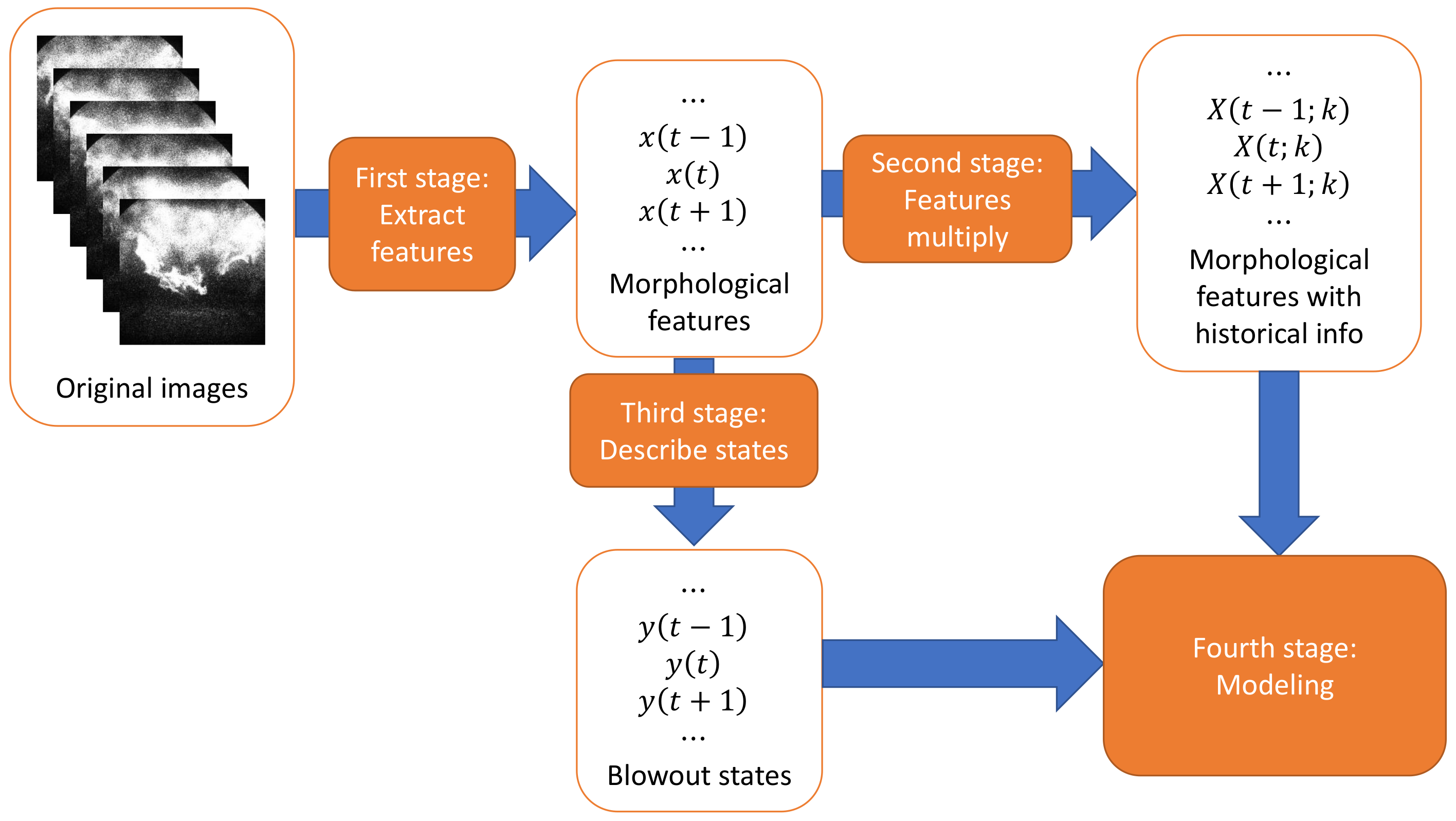
The prediction method proposed has four main stages, which are summarized in Figure 2, and described in detail in the subsequent sections. The first stage is the feature-extracting stage, in which the original flame images are processed with morphological methods so that the complicated flame images are reduced to several explainable morphological features. The second stage is the feature-multiplied stage, in which the morphological features in a certain time range are combined as the features with time series information. The third stage is the state-describing stage, in which the blowout states are defined and described numerically. The fourth and final stage is the modeling stage, where the random forest regression model is applied to build a prediction model on the LBO with the data processed before.

3.2. Extraction of Flame Morphological Features

During the oscillation process of the lean premixed flame, the flame area, and chemiluminescence intensity will change significantly. At the same time, the back-and-forth jump of the flame from the standing state to the floating state, the wrinkling of the flame edge, and the local extinguish phenomenon inside the flame are all image features that can be observed from the flame image and reflect the combustion state of the lean premixed flame. Therefore, the frequency and degree of the occurrence of the phenomena mentioned before can be captured by the feature extraction of the flame image so as to obtain the details and progress of the reacting flow process in the lean premixed combustion system. As a result, the subsequent prediction process of the flame blowout state of the lean premixed flame will have strong explainability.

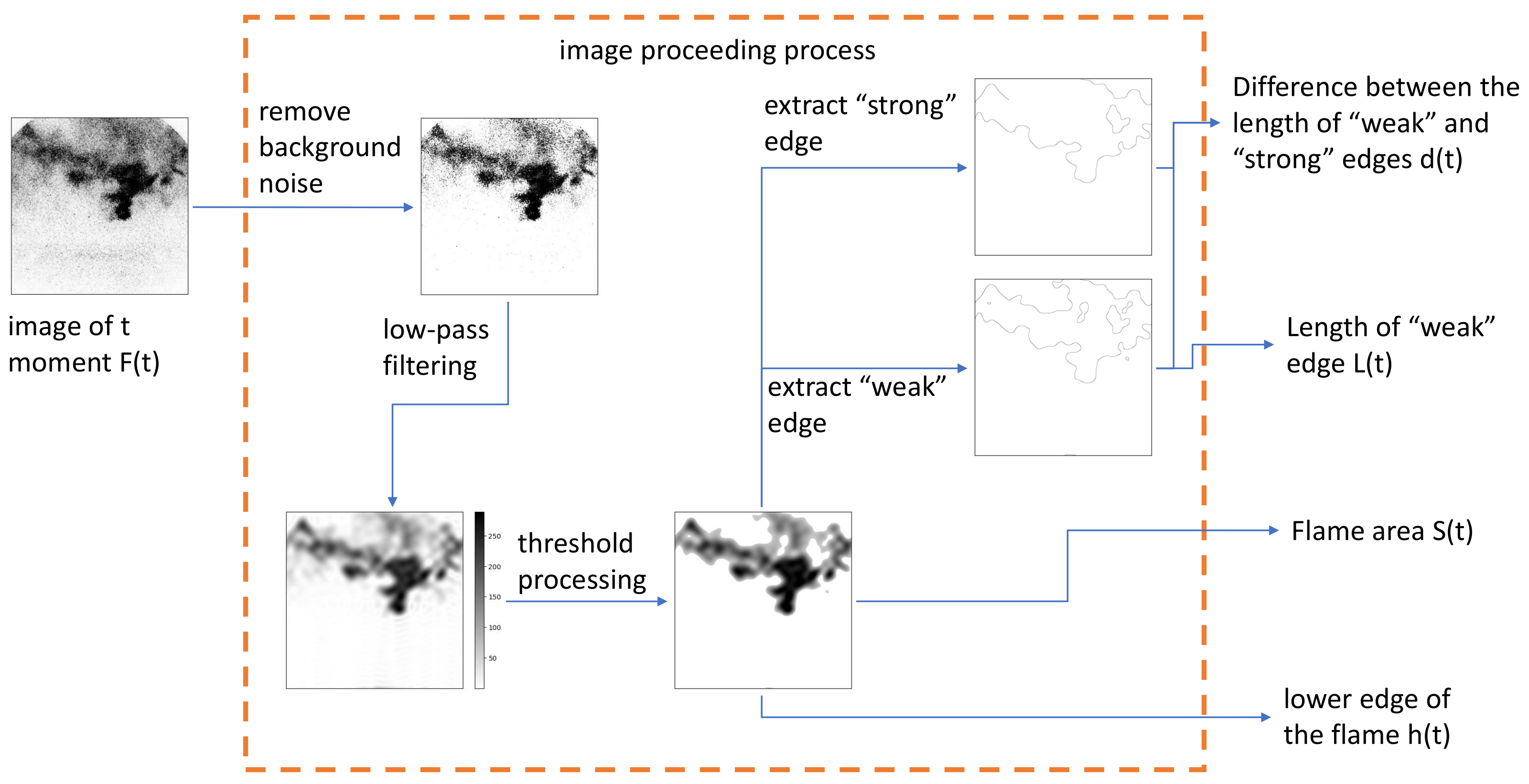
Based on the image features mentioned above, we design the experimental image processing process shown in Figure 3 and extract the required features. First, we use the threshold method to zero the pixel with a value below half to remove the background noise. Then, the image is low-pass filtered through a fast Fourier transform to convert the dot-like distribution of pixels in the area with weak light intensity into a cloud map. After that, the value range is adjusted and then the threshold truncation treatment is done again to strip out the flame area. For the obtained flame contour image, the position of the lower edge of the flame h is found by searching for the lowest point of the flame contour. The flame area S is obtained by directly summing the normalized pixel values. The flame edge extraction is carried out by using the Canny edge detection algorithm [38], where the high and low thresholds of the “strong” edge are 200 and 130, and the high and low thresholds of the “weak” edge are 130 and 20, respectively. Finally, the normalized pixel results of the obtained “strong” and “weak” edges are summed to obtain the length of the flame “weak” edge L and the difference between the length of flame “weak” and “strong” edges d.

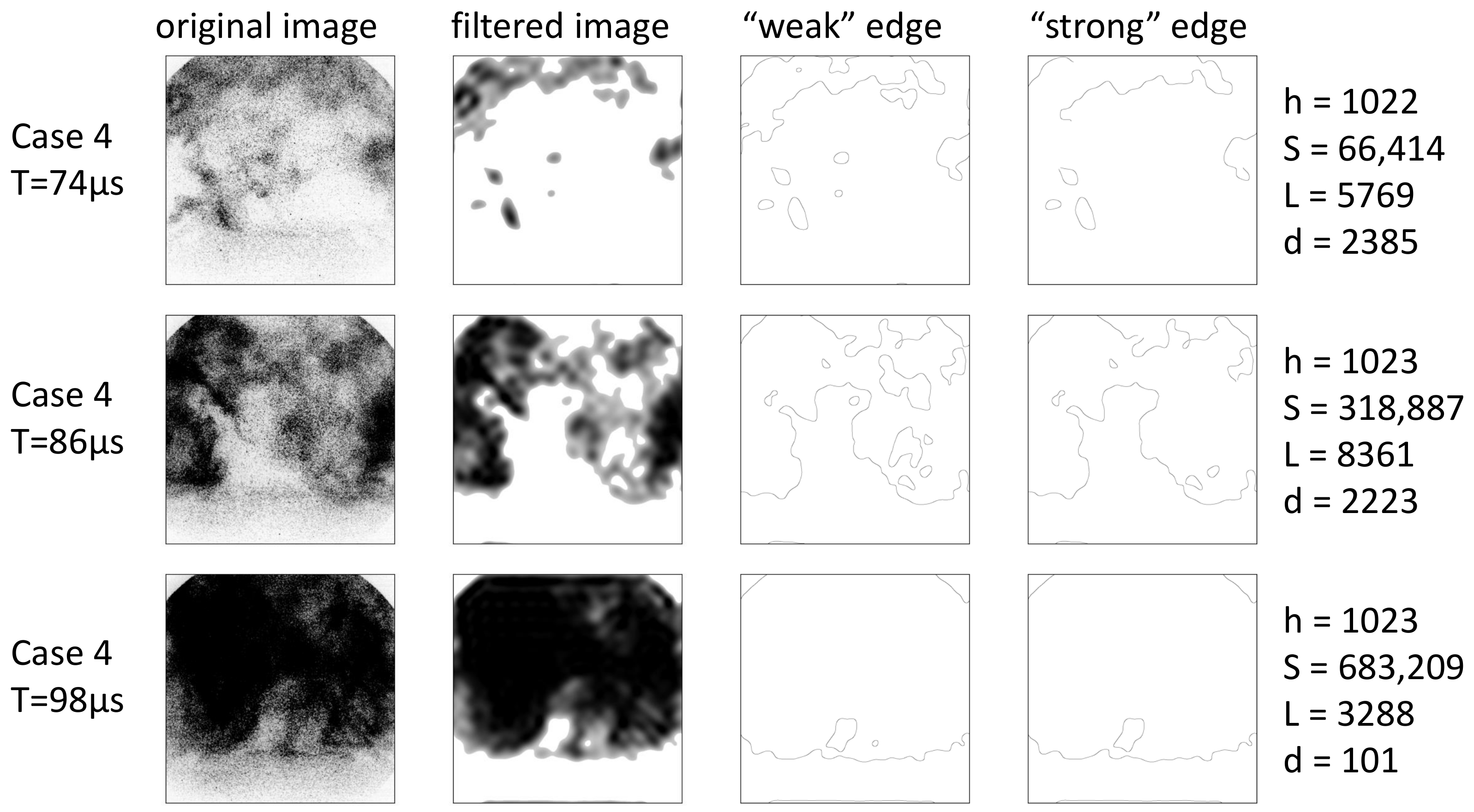
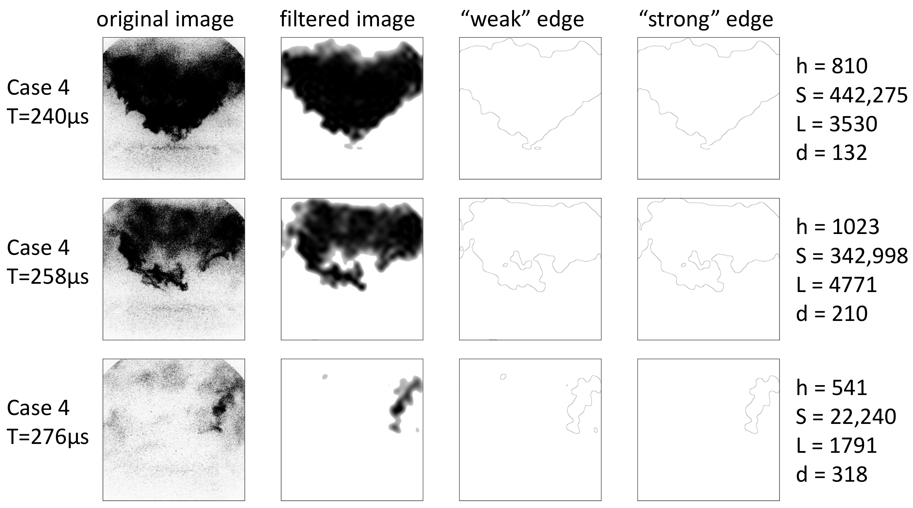
These extracted features are related to the typical phenomena that occur during the oscillation of the lean premixed flame as mentioned before. Specifically, the area and average light intensity of the flame can reflect the intensity of the overall combustion process; the position of the lower edge of the flame can reflect whether the swirling flame is standing or rising; and the “weak” edge length of the flame reflects the wrinkle of the flame edge, which in turn characterizes the degree of the flame stretch and strain rate. The difference in the length of the “strong” and “weak” edges of the flame are the embodiment of the local extinguish phenomenon inside the flame surface, which corresponds to the degree of local combustion instability. Therefore, the feature extraction of the high-frequency flame images can obtain essential information that reflects the multi-physics process of swirl combustion. In Figure 4 and Figure 5, the morphological feature extraction and the extracted feature values of some images during the reignition process and extinguish process are exhibited.

It can be seen from Figure 4 and Figure 5 that during the extinguishing process and the reignition process, the characteristics of the flame area, flame edge length, and other characteristics undergo distinctive changes. For example, during the reignition process in Figure 4, the flame area increases significantly, the flame “weak” edge length first increases and then decreases, and the difference between the flame “strong” and “weak” edge is significantly reduced. On the other hand, during the blowout process in Figure 5, the flame area is decreased significantly, the length of the “weak” edge of the flame first is increased slowly and then decreased sharply, and the difference of flame “strong” and “weak” edge is gradually increased. This means that all these image features we selected can reflect some typical processes in the process of local flame extinguishment and reignition. However, from Figure 4 and Figure 5, it can also be seen that the lowest point of the flame obtained by image processing seems to be somewhat different from the lowest point of the flame area observed by the naked eye. This may be due to inadequate image processing, and subsequent improvements may be needed.

3.3. Multiplying of Flame Morphological Features with Time Series Information

Considering that the judgment of the blowout state cannot only rely on the image features or physical characteristics of a single moment, but also refer to the changes in the previous flame form, we propose to take the time series information into account.

For an image of the t moment $F\left(t\right)$ at a certain moment, the features obtained by the image processing process can be denoted as a whole vector $x\left(t\right)={(d,L,S,h)}^{\mathbf{T}}$, while for image features containing time series information, it is denoted as a combined vector $X(t;k)={(x{\left(t\right)}^{\mathbf{T}},x{(t-1)}^{\mathbf{T}},\cdots ,x{(t-k)}^{\mathbf{T}})}^{\mathbf{T}},t\ge k$, where k is the length of the time series information, that is, the image features in the past k moments are used as the predicted features of the current image. Therefore, the accuracy of prediction can be significantly improved by expanding the features used for predicting the flame-off state from four image features of a single image to $4(k+1)$ image features containing time series information. In the modeling process, the length k of the time series information is set to 100. The influence of the time series information on the improvement of prediction accuracy is discussed further in Section 4.2.

3.4. Blowout State Description Method

It is difficult to judge whether the near-LBO swirling flame extinguishes or not because only the two states of the complete blowout and near-stable combustion can be clearly judged, while the flame state between them is difficult to judge.

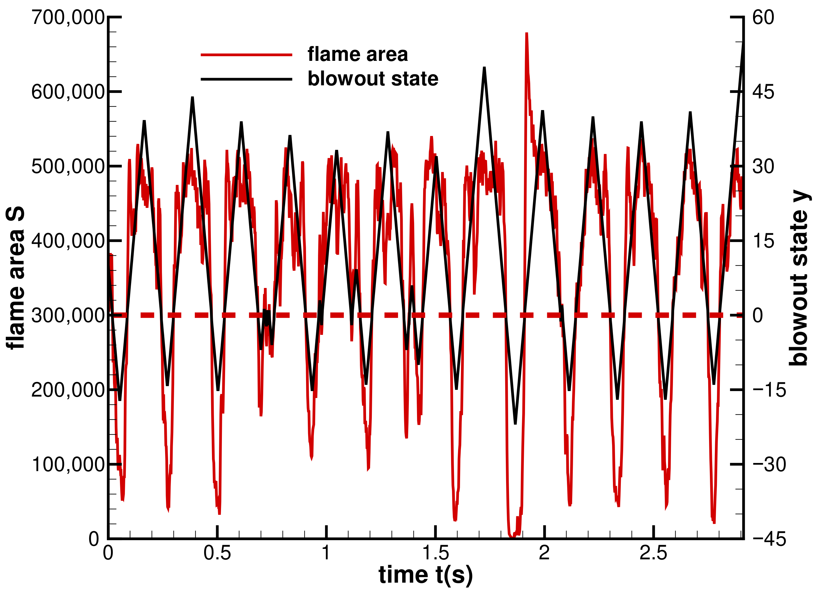
In this paper, a flame area threshold is used as the criterion for whether the flame is in a blowout state or not. Then the moments when the blowout state changes are used as “zero-nodes”. The frame spacing from the current frame to the closest “zero-nodes” is set to the value of the blowout state, and if the current state is the blowout state, a negative sign is added to the original value as the final blowout state value. This method transforms the original binary judgment problem into a numerical prediction problem so that the description of the blowout state has higher stability and statistical distribution uniformity.

This type of blowout state value also has a corresponding physical meaning, that is, when the value is positively larger, it means that the current state is farther away from the blowout state; when the value is close to zero, it means that the current state is close to blowout; and when the value is negative, a smaller value means that the current state is closer to complete extinguishment.

Figure 6 and Figure 7 exhibit the result of describing the blowout state of Cases 4 and 9 using the blowout state description method described above, in which the red dashed line is the threshold of LBO in the flame area (set to 300,000 here). The intersections of the solid red line and the dashed red line are used for estimating the value of the blowout state. It can be observed that, in this way, the originally complicated and irregular flame area change process is transformed into a blowout state change process with statistical distribution uniformity, which reduces the difficulty of modeling and improves the modeling accuracy.

3.5. Random Forest Regression Model

The random forest model is a machine learning method that uses the bootstrap method to randomly select samples from the original training set, build a CART regression tree based on these randomly selected samples, and then integrate multiple regression trees. This method has the characteristics of a simple and clear algorithm, strong practicability, good prediction accuracy, and strong noise robustness. Since its sample set selection and input feature selection are random, it can avoid the over-fitting problem in the process of model learning [39].

By using the aforementioned methods, the swirling combustion blowout prediction problem is transformed into a high-dimensional regression problem, and the random forest regression model is used to deal with the problem so as to obtain the LBO prediction model. The random forest regression model is applied directly to predict the blowout states based on the extracted features with time-series information. The input variables are the extracted features with time-series information, and the output variable is the blowout states. Taking into account the number of input samples and the number of features, we set the number of regression trees in the model to 1000. To evaluate the predictive effect of the model, we use two indicators: root mean square error (RMSE) and coefficient of determination ($R^2$). They are calculated as follows:

$$\mathrm{RMSE}=\sqrt{\frac{1}{n}\sum _{i=1}^n{({\widehat{y}}_i-y_i)}^2},$$

(1)

$$R^2=1-\frac{\sum _{i=1}^n{({\widehat{y}}_i-y_i)}^2}{{\sum }_{i=1}^n{(\overline{y}-y_i)}^2},$$

(2)

where n is the number of samples in the data set, ${\widehat{y}}_i$ is the predicted value of the model, $y_i$ is the corresponding true value, and $\overline{y}={\sum }_{i=1}^n{y}_i$ is the average of the true value.

4. Results and Discussion

4.1. Prediction Method on LBO

Four models, Models (a)–(d), are trained with different data sets selected. After the determination of the time series information length k, some images cannot be included in the data sets, due to lacking sufficient time-series information ($t<k$), complete extinction ($S=0$), and incomplete description of the blowout state ($t>t_{\mathrm{end}}$, where $t_{\mathrm{end}}$ is the last “zero-node” moment). In total, 90% of each data set is used as the training sets, and the remaining 10% is used as test sets so as to train and test Models (a)–(d). A summary of these models is listed in

Table 2. A summary of the models, with the data sets used and the performance results. $R^2$ is the coefficient of determination on the test sets, and RMSE is the root mean square error on the test sets.

Model	Cases Used	${\mathit{R}}^2$	RMSE
(a)	4	0.9890	2.64
(b)	1, 4, 7	0.9877	2.83
(c)	4–6	0.9791	3.53
(d)	1–9	0.9766	3.78

, with the data sets they used and their performances. The detailed performance results of these models are exhibited in Figure 8.

According to Figure 8, the prediction performance of each model is very good. Although the prediction accuracy of the model has decreased to a certain extent with the gradual diversification of the swirl flow conditions, it still remains at a good level. In particular, Model (d) can still have good prediction ability with unified modeling of multiple complex working conditions, indicating that it has excellent generalization performance. In addition, the model has a clear degree of differentiation near the blowout state transition. In the case of being far from the blowout state transition, the positive prediction result tends to be conservative, that is, it will be predicted lower than it actually is. This makes the model itself have a considerable prediction margin, which can reduce or even eliminate the artificial design margin in the process of applying the model.

4.2. Discussion about Influence of Time Series Information on Prediction Accuracy

Considering that the time series information is used in the prediction model to expand the data features during the construction process, and how long the time series information is used to multiply the data features is an important factor affecting the model accuracy and construction efficiency, the influence of time series information on prediction accuracy is estimated in this section. The data set used is similar to Model (d). Figure 9 exhibits how the length of the time series information affects the accuracy of Model (d) by adjusting the length of the time series information k and calculating corresponding model accuracy quantities $R^2$ and RMSE.

It is clear from Figure 9 that in general, with the increase in the length of the time series information k, the accuracy of the model is continuously improving. When k is less than 100, especially when k is less than 50, the model accuracy will improve significantly with the increase of k. However, if k is greater than 100, although there is still a certain improvement, it is minimal: the $R^2$ and the RMSE are basically stable at about 0.98 and 3.3, respectively. This means that, for the LBO prediction model proposed, the image morphological features of the past 50 frames (or 100 $\mu s$ in time) are crucial for effective prediction, and the features of the past 50th to 100th frames are also helpful for improving the prediction accuracy, but the time series information image features of more than 100 frames are not much helpful for the prediction accuracy of the LBO. Considering that with the increase in the length k of the time series information, the input dimension of the model also increases simultaneously, which in turn requires more time for model construction, so taking hyperparameter k as 100 is a good choice that takes into account the model construction accuracy and efficiency.

5. Conclusions

A novel LBO prediction method, including image feature extraction method, time series information introduction method, and blowout state description method, is proposed in this paper. It can extract features from flame images, use time series information to expand features to generate high-dimensional high-quality data, and finally predict the current blowout state value by using random forest regression model. The coefficient of determination of the model on the test set using the data of the whole working conditions reaches 0.9766, and the root mean square error is 3.78, which proves that this LBO prediction method has good generalization ability. Further study on the time series information introduction method shows that when the length of time series information is greater than 100, the accuracy of the model basically does not improve with more time series information, reflecting the insensitivity of the method on this hyperparameter.

In the future, we can further explore some other hyperparameters used in this method to expand the applicable environment of the method, and we can also try to predict the combustion flow trend of other physics information with similar properties on the basis of this set of LBO prediction methods.

References

1. Candel, S.; Durox, D.; Schuller, T.; Palies, P.; Bourgouin, J.F.; Moeck, J.P. Progress and challenges in swirling flame dynamics. Comptes Rendus Mec. 2012, 340, 758–768. [Google Scholar] [CrossRef]
2. Broda, J.; Seo, S.; Santoro, R.; Shirhattikar, G.; Yang, V. An experimental study of combustion dynamics of a premixed swirl injector. Symp. (Int.) Combust. 1998, 27, 1849–1856. [Google Scholar] [CrossRef]
3. Thiruchengode, M.; Jerry, S. Characterization of extinction events near blowout in swirl dump combustors. In Proceedings of the 41st AIAA/ASME/SAE/ASEE Joint Propulsion Conference & Exhibit, Tucson, AZ, USA, 10–13 July 2005; p. 4331. [Google Scholar]
4. Thumuluru, S.K.; Lieuwen, T. Characterization of acoustically forced swirl flame dynamics. Proc. Combust. Inst. 2009, 32, 2893–2900. [Google Scholar] [CrossRef]
5. Lacarelle, A.; Faustmann, T.; Greenblatt, D.; Paschereit, C.; Lehmann, O.; Luchtenburg, D.; Noack, B. Spatiotemporal characterization of a conical swirler flow field under strong forcing. J. Eng. Gas Turbines Power 2009, 131, 031504. [Google Scholar] [CrossRef] [Green Version]
6. Steinberg, A.M.; Boxx, I.; Stöhr, M.; Carter, C.D.; Meier, W. Flow–flame interactions causing acoustically coupled heat release fluctuations in a thermo-acoustically unstable gas turbine model combustor. Combust. Flame 2010, 157, 2250–2266. [Google Scholar] [CrossRef] [Green Version]
7. Stöhr, M.; Boxx, I.; Carter, C.; Meier, W. Dynamics of lean blowout of a swirl-stabilized flame in a gas turbine model combustor. Proc. Combust. Inst. 2011, 33, 2953–2960. [Google Scholar] [CrossRef] [Green Version]
8. Chterev, I.; Foley, C.; Foti, D.; Kostka, S.; Caswell, A.; Jiang, N.; Lynch, A.; Noble, D.; Menon, S.; Seitzman, J.; et al. Flame and flow topologies in an annular swirling flow. Combust. Sci. Technol. 2014, 186, 1041–1074. [Google Scholar] [CrossRef]
9. Zhang, W.; Wang, J.; Guo, S.; Chang, M.; Nie, Y.; Jin, W.; Huang, Z. Study on flame structure of lean premixed CH4/air flames close to blow-off. J. Combust. Sci. Technol. 2019, 25, 389–394. [Google Scholar]
10. Zhao, X.; Ge, H.; Wang, J.; Xu, W.; Zhou, Y. Blow-out mechanism of lean-premixed swirl flame combustion based on flame OH chemiluminescence technology. J. Combust. Sci. Technol. 2019, 25, 244–250. [Google Scholar]
11. Huang, Y.; Sung, H.G.; Hsieh, S.Y.; Yang, V. Large-eddy simulation of combustion dynamics of lean-premixed swirl-stabilized combustor. J. Propuls. Power 2003, 19, 782–794. [Google Scholar] [CrossRef] [Green Version]
12. Huang, Y.; Yang, V. Bifurcation of flame structure in a lean-premixed swirl-stabilized combustor: Transition from stable to unstable flame. Combust. Flame 2004, 136, 383–389. [Google Scholar] [CrossRef]
13. Boileau, M.; Staffelbach, G.; Cuenot, B.; Poinsot, T.; Bérat, C. LES of an ignition sequence in a gas turbine engine. Combust. Flame 2008, 154, 2–22. [Google Scholar] [CrossRef] [Green Version]
14. Boxx, I.; Stöhr, M.; Carter, C.; Meier, W. Temporally resolved planar measurements of transient phenomena in a partially pre-mixed swirl flame in a gas turbine model combustor. Combust. Flame 2010, 157, 1510–1525. [Google Scholar] [CrossRef] [Green Version]
15. Palies, P.; Schuller, T.; Durox, D.; Gicquel, L.; Candel, S. Acoustically perturbed turbulent premixed swirling flames. Phys. Fluids 2011, 23, 037101. [Google Scholar] [CrossRef] [Green Version]
16. Huang, Y.; Yang, V. Dynamics and stability of lean-premixed swirl-stabilized combustion. Prog. Energy Combust. Sci. 2009, 35, 293–364. [Google Scholar] [CrossRef]
17. Candel, S.; Durox, D.; Schuller, T.; Bourgouin, J.F.; Moeck, J.P. Dynamics of swirling flames. Annu. Rev. Fluid Mech. 2014, 46, 147–173. [Google Scholar] [CrossRef]
18. Yu, S.; Liu, X.; Liu, X.; Zhang, Z. Prototype swirl flame using strained flamelet generated manifold. J. Combust. Sci. Technol. 2020, 26, 301–309. [Google Scholar]
19. Huang, J.; Li, L.; Cai, W. Experimental prediction of lean blowout: A review. J. Exp. Fluid Mech. 2018, 32, 1–9. [Google Scholar]
20. Thiruchengode, M.; Nair, S.; Neumeier, Y.; Lieuwen, T.; Seitzman, J.; Zinn, B.; Jagoda, J.; Scarborough, D.; Coker, A. An active control system for LBO margin reduction in turbine engines. In Proceedings of the 41st Aerospace Sciences Meeting and Exhibit, Reno, Nevada, 6–9 January 2003; p. 1008. [Google Scholar]
21. Nair, S.; Lieuwen, T.; Thiruchengode, M.; Seitzman, J.; Meyers, A.; Zinn, B. Lean Blowout Detection in a Single Nozzle Swirl Cup Combustor. In Proceedings of the 42nd AIAA Aerospace Sciences Meeting and Exhibit, Reno, Nevada, 5–8 January 2004; p. 138. [Google Scholar]
22. Thiruchengode, M. Sensing and Dynamics of Lean Blowout in a Swirl Dump Combustor. Ph.D. Thesis, Georgia Institute of Technology, Atlanta, GA, USA, 2006. [Google Scholar]
23. Huang, H.W.; Zhang, Y. Flame colour characterization in the visible and infrared spectrum using a digital camera and image processing. Meas. Sci. Technol. 2008, 19, 085406. [Google Scholar] [CrossRef]
24. Chaudhari, R.R.; Sahu, R.P.; Ghosh, S.; Mukhopadhyay, A.; Sen, S. Flame color as a lean blowout predictor. Int. J. Spray Combust. Dyn. 2013, 5, 49–65. [Google Scholar] [CrossRef] [Green Version]
25. Bompelly, R.; Lieuwen, T.; Seitzman, J. Lean blowout and its sensing in the presence of combustion dynamics in a premixed swirl combustor. In Proceedings of the 47th AIAA Aerospace Sciences Meeting Including The New Horizons Forum and Aerospace Exposition, Orlando, FL, USA, 5–8 January 2009; p. 982. [Google Scholar]
26. Yi, T.; Gutmark, E.J. Real-time prediction of incipient lean blowout in gas turbine combustors. AIAA J. 2007, 45, 1734–1739. [Google Scholar] [CrossRef]
27. Zhou, L.; Song, Y.; Ji, W.; Wei, H. Machine learning for combustion. Energy AI 2022, 7, 100128. [Google Scholar] [CrossRef]
28. Sarkar, S.; Lore, K.G.; Sarkar, S. Early Detection of Combustion Instability by Neural-Symbolic Analysis on Hi-Speed Video. In Proceedings of the CoCo@ NIPS, Montreal, QC, Canada, 11–12 December 2015. [Google Scholar]
29. Wang, Z.; Song, C.; Chen, T. Deep learning based monitoring of furnace combustion state and measurement of heat release rate. Energy 2017, 131, 106–112. [Google Scholar] [CrossRef]
30. Tokarev, M.; Abdurakipov, S.; Gobyzov, O.; Seredkin, A.; Dulin, V. Monitoring of combustion regimes based on the visualization of the flame and machine learning. Proc. J. Phys. Conf. Ser. 2018, 1128, 012138. [Google Scholar] [CrossRef] [Green Version]
31. Akintayo, A.; Lore, K.G.; Sarkar, S.; Sarkar, S. Early detection of combustion instabilities using deep convolutional selective autoencoders on hi-speed flame video. arXiv 2016, arXiv:1603.07839. [Google Scholar]
32. Akintayo, A.; Lore, K.G.; Sarkar, S.; Sarkar, S. Prognostics of combustion instabilities from hi-speed flame video using a deep convolutional selective autoencoder. Int. J. Progn. Health Manag. 2016, 7. [Google Scholar] [CrossRef]
33. Qiu, T.; Liu, M.; Zhou, G.; Wang, L.; Gao, K. An unsupervised classification method for flame image of pulverized coal combustion based on convolutional auto-encoder and hidden Markov model. Energies 2019, 12, 2585. [Google Scholar] [CrossRef] [Green Version]
34. Han, X.; Laera, D.; Morgans, A.; Sung, C.; Hui, X.; Lin, Y. Flame macrostructures and thermoacoustic instabilities in stratified swirling flames. Proc. Combust. Inst. 2019, 37, 5377–5384. [Google Scholar] [CrossRef] [Green Version]
35. Han, X.; Laera, D.; Morgans, A.S.; Lin, Y.; Sung, C.J. The effect of stratification ratio on the macrostructure of stratified swirl flames: Experimental and numerical study. J. Eng. Gas Turbines Power 2018, 140, 121004. [Google Scholar] [CrossRef]
36. He, T.; Wang, S.; Liu, X.; Li, L.; Han, X.; Zhang, C.; Dong, X.; Qi, F. Prediction method and experimental research on lean burn blow-off based on deep learning. J. Combust. Sci. Technol. 2022, 28, 304–312. [Google Scholar]
37. Wang, S.; Liu, X.; Li, L.; Han, X.; Zhang, C.; Qi, F. Effects of stratification ratio on flame stabilization and flow structure in stratified swirling flame. Acta Aerodyn. Sin. 2020, 38, 619–628. [Google Scholar]
38. Canny, J. A computational approach to edge detection. IEEE Trans. Pattern Anal. Mach. Intell. 1986, PAMI-8, 679–698. [Google Scholar] [CrossRef]
39. Breiman, L. Random forests. Mach. Learn. 2001, 45, 5–32. [Google Scholar] [CrossRef] [Green Version]
Figure 1. Scheme of BASIS swirler and CH chemiluminescence experiment system [34].
Applsci 13 03173 g001
Figure 2. A flow chart of the prediction method. x ( t ) is the extracted morphological feature vector at the t moment, X ( t ; k ) is the combined morphological feature vector with the information of the k length time series, and y ( t ) is the corresponding blowout state.
Applsci 13 03173 g002
Figure 3. Experimental image processing process and corresponding features acquired.
Applsci 13 03173 g003
Figure 4. Morphological feature extraction results from images during reignition process.
Applsci 13 03173 g004
Figure 5. Morphological feature extraction results from images during blowout process.
Applsci 13 03173 g005
Figure 6. Temporal evolution of flame area S (red line with the left scale) and corresponding blowout state value (black line with the right scale) in Case 4 mentioned in Table 1.
Applsci 13 03173 g006
Figure 7. Temporal evolution of flame area S (red line with the left scale) and corresponding blowout state value (black line with the right scale) in Case 9 mentioned in Table 1.
Applsci 13 03173 g007
Figure 8. Performances of the prediction models with different data sets. Each red points represents the model prediction value and corresponding true value of a data, the abscissa represents the true value, and the ordinate represents the predicted value. Black line is the reference line where the prediction values and corresponding true values are equal, respectively. (a) performance of Model (a); (b) performance of Model (b); (c) performance of Model (c); (d) performance of Model (d).
Applsci 13 03173 g008
Figure 9. The effect of the length of the time series information used by the LBO prediction model on the accuracy of Model (d). The red line with circles shows the R 2 results with the left scale. The green line with diamonds shows the RMSE results with the right scale.
Applsci 13 03173 g009