Article

Reactor Temperature Prediction Method Based on CPSO-RBF-BP Neural Network

1
School of Electrical and Electronic Engineering, Shanghai Institute of Technology, Shanghai 201418, China
2
Engineering Management, Melbourne University, Melbourne 3128, Australia
*
Author to whom correspondence should be addressed.
Appl. Sci. 2023, 13(5), 3230; https://doi.org/10.3390/app13053230
Submission received: 30 January 2023 / Revised: 25 February 2023 / Accepted: 25 February 2023 / Published: 2 March 2023
(This article belongs to the Special Issue Intelligent Control in Industrial Processes)

Abstract

:
A neural network model based on a chaotic particle swarm optimization (CPSO) radial basis function-back propagation (RBF-BP) neural network was suggested to improve the accuracy of reactor temperature prediction. The training efficiency of the RBF-BP neural network is influenced to some degree by the large randomness of the initial weight and threshold. To address the impact of initial weight and threshold uncertainty on the training efficiency of the RBF-BP combined neural network, this paper proposes using a chaotic particle swarm optimization algorithm to correct the RBF-BP neural network’s initial weight and threshold, as well as to optimize the RBF-BP neural network to speed up the algorithm and improve prediction accuracy. The measured temperature of the reactor acquired by on-site enterprises was confirmed and compared to the predicted results of the BP, RBF-BP, and PSO-RBF-BP neural network models. Finally, Matlab simulation tests were performed, and the experimental data revealed that the CPSO-RBF-BP combined neural network model suggested in this paper had a root-mean-square error of 17.3%, an average absolute error of 11.4%, and a fitting value of 99.791%. Prediction accuracy and efficiency were superior to those of the BP, RBF-BP, and PSO-RBF-BP models. The suggested model’s validity and feasibility were established. The study findings may provide some reference values for the reactor’s temperature prediction.

1. Introduction

Because of the complex reactor production process, it is difficult to establish an accurate mathematical model for most real industrial control systems, and the reactor temperature is difficult to control due to the reactor’s complex structure, physical exothermic reaction, external environment interference, and other unstable factors. The temperature of the reactor is challenging to control because the temperature of the reactor has two reaction processes: a reaction heating stage and heat release. The temperature properties of the two reactions are opposed. If excess heat is not removed during the reaction process, the temperature in the reactor will become too high, affecting product quality and manufacturing safety. If you remove too much heat, the product will respond too slowly, and it will not be qualified. As can be seen, precise reactor temperature control is closely related to product quality and production safety. Furthermore, the enterprise’s reactor capacity is generally large, resulting in a thick reactor wall, heat release, and heat absorption of the reaction process, and with the progress of the reaction process, the irregular change of the heat conducting medium is also very sensitive to external influence. The reaction kettle is a nonlinear, large hysteresis-controlled object for these systems. The temperature control of reactors has always been the emphasis and challenge of chemical enterprises in recent years. This subject has great research value because the temperature of the reactor affects not only the quality of pharmaceuticals but also the life safety of workers in enterprises. The reaction kettle in these setups is a nonlinear, massive hysteresis-regulated entity. To manage the temperature of the reactor, complex control procedures are required due to its temperature control characteristics, which include a high lag, delay, and nonlinearity. Research on how to increase the temperature control effect of reactors is increasingly becoming a topic of increasing difficulty and interest due to the increasing production quality needs of modern businesses. In recent years, numerous researchers have suggested numerous predictive control algorithms based on nonlinear models, such as the Wiener model [1,2], the neural network model [3], and the support vector machine model [4,5]. Based on these models applied to the temperature management of reactors, favorable results have been obtained. Currently, there are numerous studies on the prediction of neural networks. Liu et al. [6] used the back propagation neural network based on the particle swarm optimization algorithm to study the prediction of the high-speed grinding temperature of titanium matrix composites, and verified through experiments that the PSO-BP method has more advantages over other methods in predicting grinding temperature in terms of convergence rate, fitting accuracy, and prediction accuracy. Liu et al. [7] proposed a multi-variable prediction method for short-term power loads based on chaos theory and a radial basis function neural network and found through experimental data that this method significantly improved the accuracy of prediction. Zhang et al. [8] proposed a method to optimize the BP neural network by using a chaotic particle swarm optimization algorithm to improve the prediction accuracy of PM2.5 concentration in the atmosphere. The results show that the CPSO-BP neural network has better prediction performance than the traditional BP neural network. Yang [9] proposed an improved radial basis function neural network model based on CPSO to solve the nonlinear control problem. The results showed that the model had obvious advantages in drug saving, small overshooting, and shortened adjustment time, thus achieving the lowest cost effect. Wu et al. [10] proposed a model based on the improved Sparrow algorithm to optimize the RBF-BP neural network. Through the analysis of simulation experiment results, the LISSA-RBF-BP model can predict the gold tungsten powder stock more accurately than the RBF-BP model and the SSA-RBF-BP model. Li et al. [11] used BP and RBF neural networks to make a short-term prediction of SST, and the results showed that both the BP and RBF neural networks could effectively predict the seasonal changes of SST data, but the overall prediction effect of the RBF neural network was better than that of the BP neural network for different prediction times. In addition to the study described above, neural networks can be applied to other types of research [12,13,14,15,16].
This paper suggested the RBF-BP neural network model based on a chaotic particle swarm optimization algorithm to forecast the temperature of the reactor, based on the theoretical foundation of the above scholars’ research. By correcting the initial weight and threshold of the RBF-BP neural network with a chaotic particle swarm optimization algorithm, the neural network can effectively avoid falling into the local optimal solution and improve the convergence rate, thereby improving the prediction accuracy of reactor temperature. The model was tested against the BP, RBF-BP, and PSO-RBF-BP algorithms. The simulation results indicate that the CPSO-RBF-BP model predicts the reactor temperature more accurately and with less error. The remainder of this document will be organized as follows: Section 2 describes the RBF-BP neural network model’s structure and content, as well as the temperature prediction algorithm of the CPSO-RBF-BP reactor. The contrast of four neural networks for temperature prediction is summarised and analyzed in Section 3. Section 4 summarises the paper’s work substance.

2. RBF-BP Combined Neural Network Model

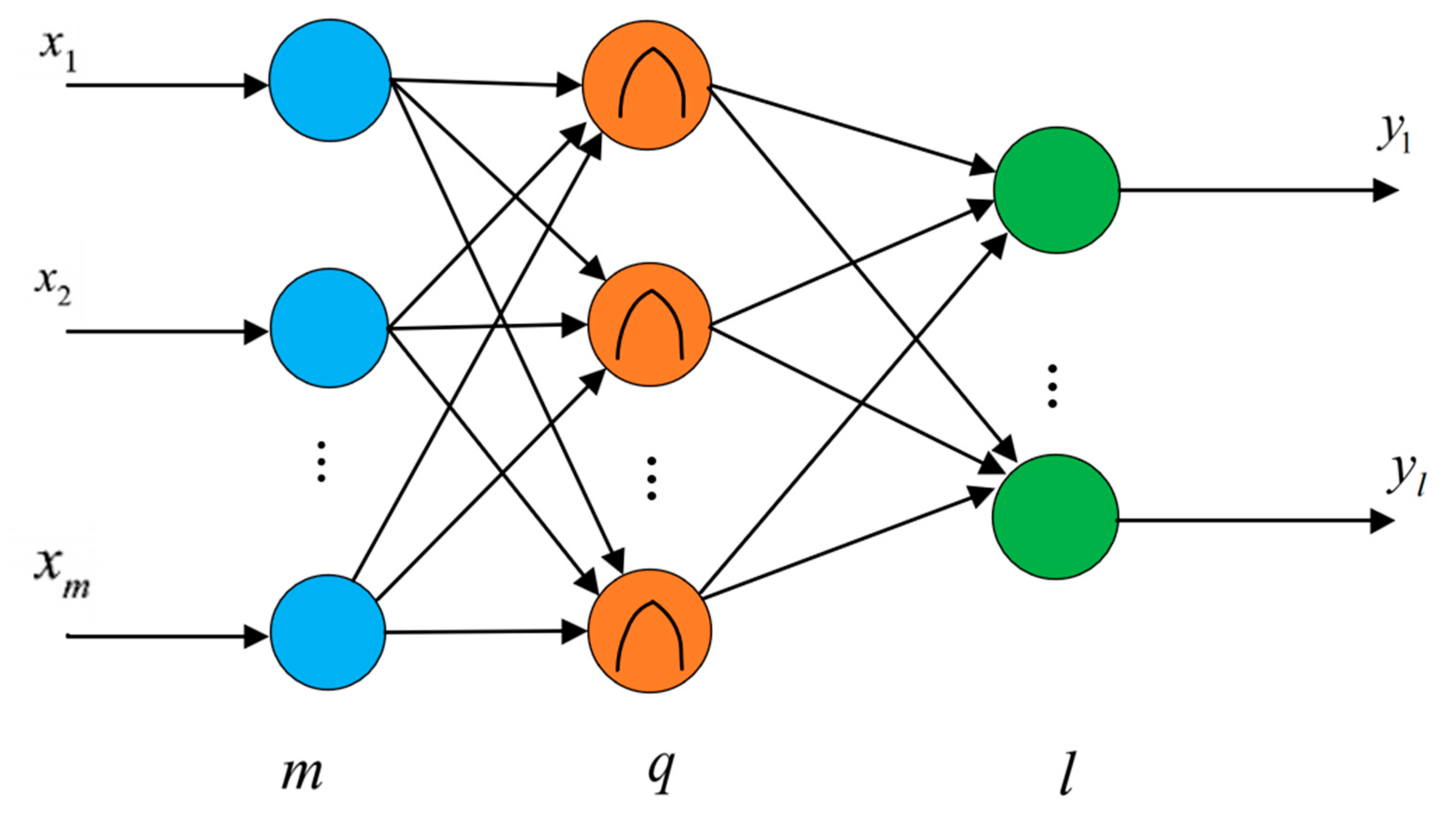
2.1. RBF Neural Network

Figure 1 depicts the layout of the RBF neural network, which consists of three layers: m inputs, q hidden layers, and 1 output. The first input layer is used to transfer input variables to the hidden layer, which is composed of basis functions. As the overall output, the output layer is a linear mapping of the implicit layer’s output. RBF neural networks offer a robust nonlinear approximation capability and a robust self-learning capability, allowing them to demonstrate good self-adaptive capabilities in the face of varied environmental changes. Industrial process control increasingly employs RBF neural networks [17].

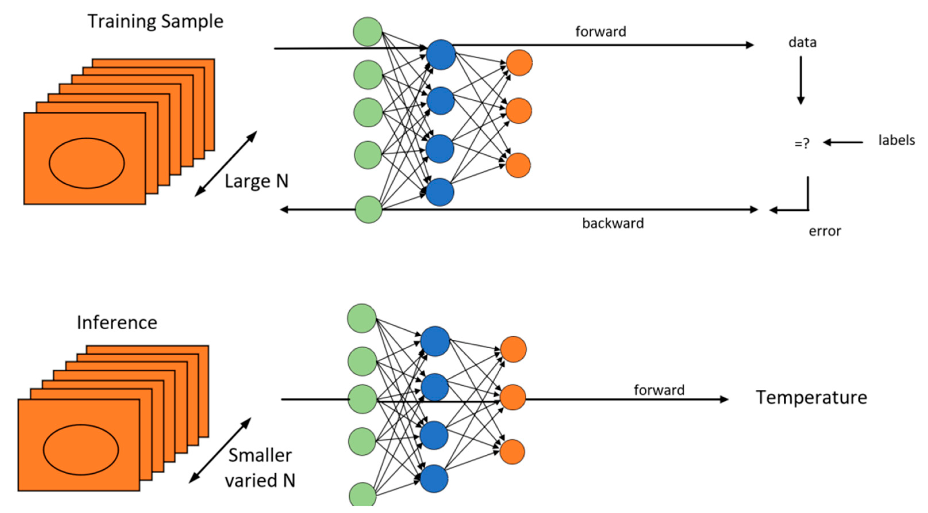
2.2. BP Neural Network

In both theory and practice, the BP algorithm has reached a more general applicability in some nonlinear predictions [18]. The learning process consists of two processes: forward propagation of the signal, and backward propagation of the error. Forward propagation is the consequence of feeding training data to the input layer, which is computed layer by layer by the neural network. Backpropagation is accomplished by backpropagating the error to all the units in each layer using the error values to update the iterative solution weight and bias term values [19]. However, this technique has certain unresolved flaws, and its algorithm uses gradient descent as a training method, resulting in a propensity for local optima [20]. Figure 2 depicts the optimum neural network diagram for BP. The BP algorithm is composed of input, hidden, and output layers which belong to the multi-level feedforward neural network. The main feature of the network is that it needs to go through multiple forward propagation networks, and the error is propagated back. The idea is to input a set of samples to achieve the output by calculation, and then to get the difference between the actual output and the expected value to continuously adjust the weight and threshold to minimize the difference. The process is repeated until the difference is less than a predetermined value. In the forward pass, the input layer passes through multiple hidden layers to the output layer. If the output layer cannot get the expected output, it will turn to backpropagation and adjust the network weight and threshold according to the prediction error, so that the predicted output of the BP neural network is close to the expected output.

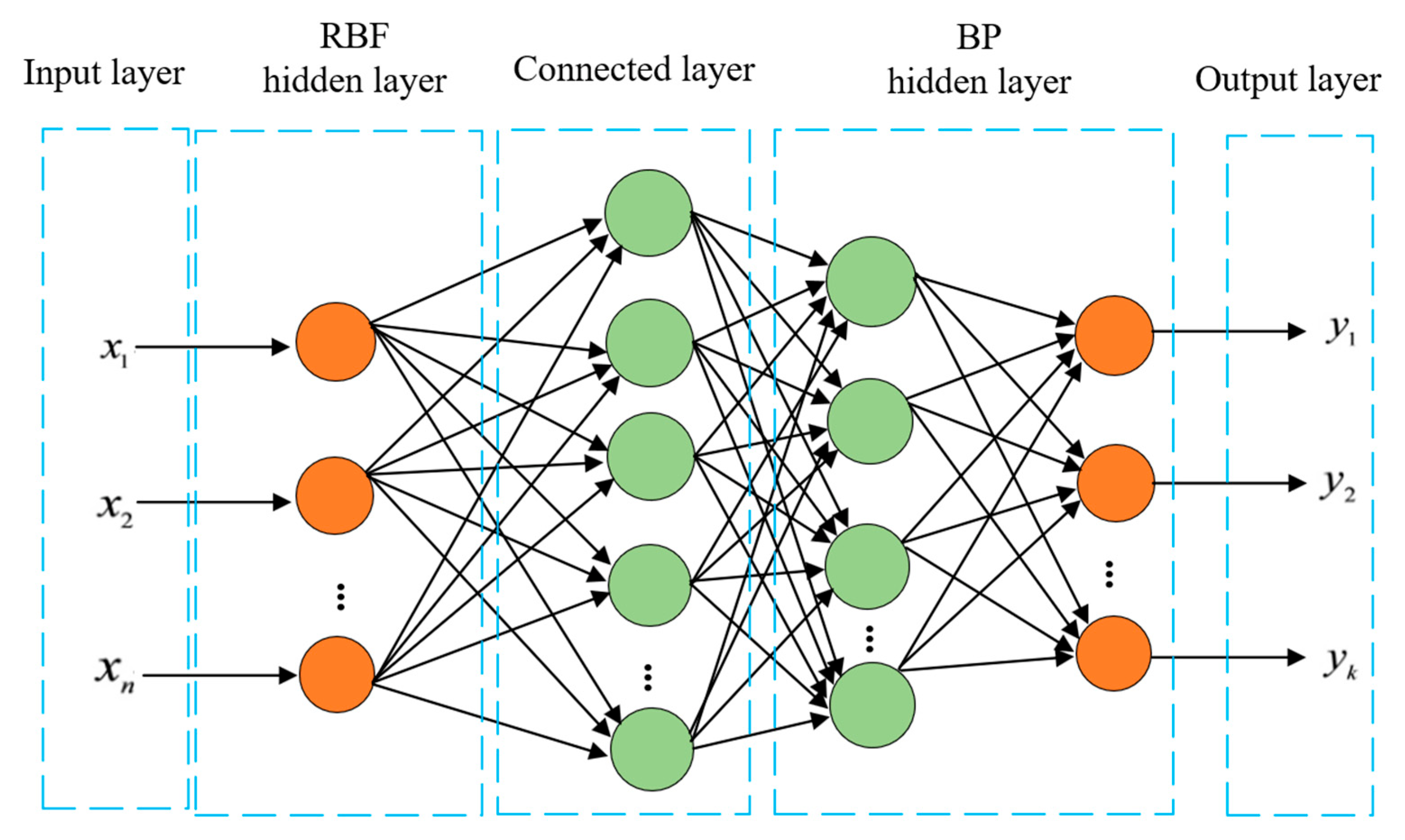
2.3. RBF-BP Neural Network

Because of their superior nonlinear prediction capability, robustness, and fault tolerance, RBF-BP neural networks are frequently used for nonlinear prediction. RBF-BP is a double-implicit neural network system composed of RBF and BP subnets that take advantage of the advantages of both neural networks. In terms of sample prediction ability, BP neural networks outperform RBF neural networks [21,22]. The combined network can also compensate for the BP neural network’s flaws, which are locally optimal solutions and slow convergence [23]. Figure 3 shows the RBF-BP hybrid neural network’s structure and network mechanism. The output of the RBF neural network acts as the input layer of the BP neural network, and this layer can also serve as the hybrid neural network’s connection layer. The output layer of the hybrid neural network is the output layer of the BP neural network. Setting up the connection layer allows them to quickly and effectively reinforce their connection, which improves the nonlinear mapping’s ability to fit.
The mixed neural network algorithm consists of two processes: forwards propagation, which propagates the error between the network and the desired output layer by layer, and backward propagation, which propagates the error between the network and the desired output from the output to the input layer, and calculates the weights according to a certain rule. The difference between the real output and the intended output can be reduced by repeated forwards and backward propagation to meet the specifications.
The overall RBF-BP neural network is completed by the following six steps.
Step 1: Initialize the weights and thresholds of each layer to (0, 1) and configure settings including the maximum number of iterations, the desired minimal error, and the learning rate.
Step 2: Assign a Gaussian basis function with the following form to the transfer function of the implied layer of the RBF subnetwork.
φ j x = e x p x c j 2 σ 2 j ,   j = 1 , 2 , , N
  j is the number of nodes, φ is the node output, x is the sample vector, c is the center of the Gaussian basis function, and σ is the width of the basis function.
Step 3: Assign a sigmoid-type function to the BP hidden layer’s transfer function.
F y = 1 / 1 + e y
Its output function is v t = F [ Σ j = 1 N 2 β 2 , t ( j ) u ( j ) ] , where N 2 represents the number of nodes in layer 2 hidden layer.
Step 4: Compute the layer output node m.
Step 5: Calculate the output layer SSE error sum of squares.
S S E = Σ o = 1 N 3 T o Y o 2
T o represents the desired output value.
Step 6: Modify the individual thresholds and weights.
β i , o = β i , o + α Y o 1 Y o T o Y o Y o  
θ o = θ o + α Y o 1 Y o T o Y o  
The procedure converges and training is completed when the training error of the merged neural network is less than the target error. When the number of training iterations exceeds the maximum number selected and the target error is not met, the algorithm returns to step 2 and executes the procedure until the entire process converges.

2.4. Algorithm for Chaotic Particle Swarm (CPSO)

(1)
Particle swarm method
The particle swarm optimization algorithm [24,25] (PSO) was inspired by a new swarm intelligence optimization technique that models animal foraging behavior, such as that of birds [26]. Its main characteristics are fast convergence, good global search capabilities, and the capacity to overcome system lag. Based on the research on the predation behavior of birds, the strategy of birds in searching for food is to find the nearest bird range to the food. These birds are called “particles”, and the particles have their position and speed. Each particle will follow the optimal particle to search in space. The idea that each particle can share the current search result is very simple and easy to implement. However, the disadvantage of PSO is that it is easy to converge quickly, so there will be a disadvantage of low accuracy. If the coefficient is accelerated, the particle easily misses the optimal solution. If, in the process of convergence, all the particles fly to the optimal solution, the particles will lose diversity and will slow down. It can locate persons who satisfy the conditions by constantly changing its search mode in the solution space [27]. A set of particles is generated at random, and each particle represents a viable solution to the problem, each particle has its fitness, and fitness determines the degree of superiority and inferiority. Throughout the solution process, the particle will continuously update its velocity and position based on the individual and global extremes to find the best solution.
V i d k + 1 = V i d k + c 1 × r 1 × P i d k X i d k + c 2 × r 2 × P g d k X i d k X i d k + 1 = X i d k + V i d k + 1
where: i = 1 , 2 , , N ; d = 1 , 2 , , M .   K is the number of iterations; c 1 and   c 2 are learning factors; And r 1 , r 2 is a random number between.
(2)
Algorithm for chaotic particle swarm
To avoid the standard particle swarm algorithm sliding into local optimality and premature aging [28], the system can be modified to show chaotic features by adding the update adjustment process of particle velocity using the chaotic algorithm’s ergodicity and regularity. The chaotic particle swarm algorithm (CPSO) seeks to achieve global optimization by substituting a chaotic sequence for the normal random sequence.
The basic idea of the CPSO is as follows:
  • Chaotic initializes the particle positions in the population. Based on the chaotic motion characteristics, selecting individuals with high fitness as the initial population can improve search efficiency.
  • Carry out a chaotic search on the top 20% of the population with high fitness, generate the corresponding chaotic sequence through Logistic mapping, and the search can be carried out in the field. Once there is a better individual extremum position, the local search ability of the algorithm can be improved by replacing it.
  • To improve the optimization performance of the algorithm, the main parameter selection and method of the algorithm were improved. In this paper, the inertia weight was linearly decreased, which can have a strong optimization ability in the early stage and can be carefully searched locally in the later stage. The formula is as follows:
ω max represents the maximum value of the weight factor, ω min represents the minimum value, the maximum value is usually 0.9, the minimum value is 0.4, t and t max are the current iterations and the maximum iteration times.
Logistic mapping formula: z t + 1 = μ z t ( 1 z t )
μ is the control variable, z t is the chaotic sequence.
In the chaotic search process, the top 20% excellent particles need to be mapped to the interval of [0, 1] of the logistic equation, and then iteratively searched by the Logistic equation to obtain the corresponding chaotic sequence and retain the feasible solution with the best performance.
Figure 4 shows the step flow of chaotic particle swarm optimization algorithm, the specific implementation steps of the CPSO algorithm are as follows:
Step 1: Initially, the population is started to define the population size N, the maximum number of chaotic iterations M, inertia weights W, learning factors c 1 ,   c 2 , and other crucial characteristics.
Step 2: Chaos sets the particle position, generates the particle using the logistic map, and chooses the particle with the highest fitness function value as the beginning population.
Step 3: The particle velocity and location of the population are updated using the particle’s iterative updating formula, the particle’s fitness is computed, and the particle’s current ideal position and global optimum are recorded.
Step 4: The top 20% of the population is chosen for chaotic search, and the particle components are then transformed to the interval [0, 1] using the formula. G repetitions of the formula yield the chaotic sequence, after which the scale is converted and the P and G of each particle are updated.
Step 5: Determine whether the maximum number of iterations of chaos has been reached; if not, return to step 3.

2.5. CPSO-RBF-BP Reactor Temperature Model Construction

The BP neural network has the issue of easily settling on a local optimal solution, which prevents it from achieving a temperature prediction effect. The CPSO-RBF-BP neural network model is created utilizing the complementing benefits of the RBF-BP combinatorial neural network and the chaotic particle swarm algorithm as a remedy to the drawbacks of the BP neural network. The precise procedures for developing the RBF-BP mixed neural network model using CPSO optimization are outlined in this study. The flow chart of steps is shown in Figure 5.
Step 1: Determine the structure of the RBF-BP combined neural network, choose five important factors affecting reactor temperature as input eigenvalues, choose temperature as the output, set the number of nodes in the input layer to 5, the number of nodes in the hidden layer to 8, and the number of output nodes to 1.
Step 2: The temperature data of Hengdian Chemical Enterprise’s reaction kettle in normal production was gathered and processed consistently, and then distributed [0, 1].
Step 3: Begin the chaotic particle swarm by determining the population size N, the maximum number of chaotic iterations M, the inertia weight, the learning factors C1 and C2, and other essential parameters.
Step 4: To determine the global optimal fitness and optimal position, the fitness of each PSO individual was calculated and sorted.
Step 5: The output is replaced by the new solution after the global optimal solution has been chaotically iterated.
Step 6: Determine whether or not the termination condition has been met. If the termination condition is met, the weight and threshold value are output; otherwise, step 4 is repeated.
Step 7: Set the output weight and threshold for the RBF-BP neural network.
Step 8: Samples were used to train the RBF-BP neural network, and the prediction accuracy was checked.

3. Analysis of Predicted Reactor Temperature

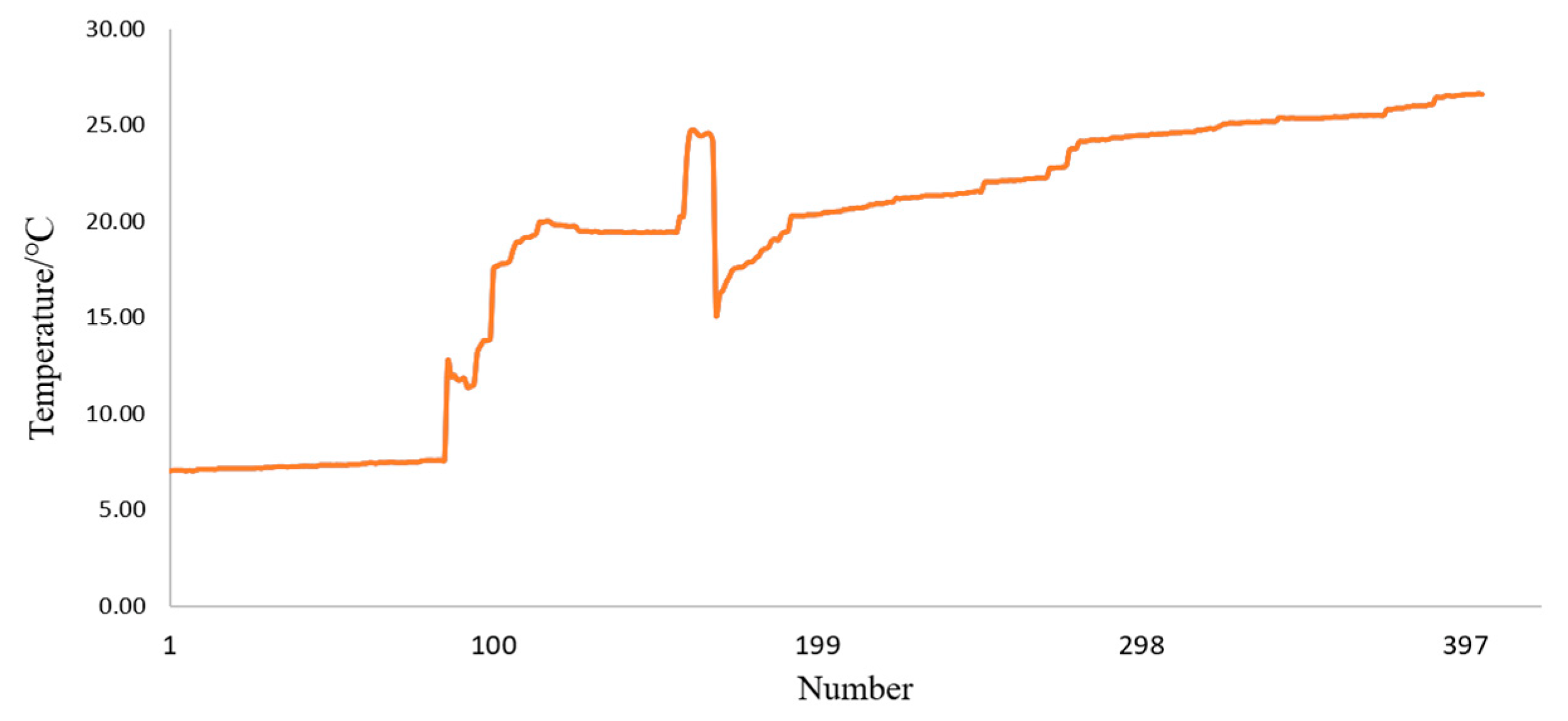
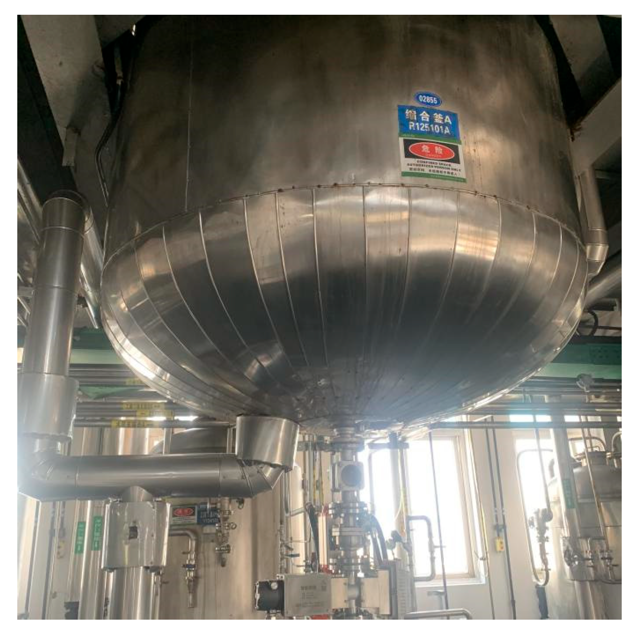
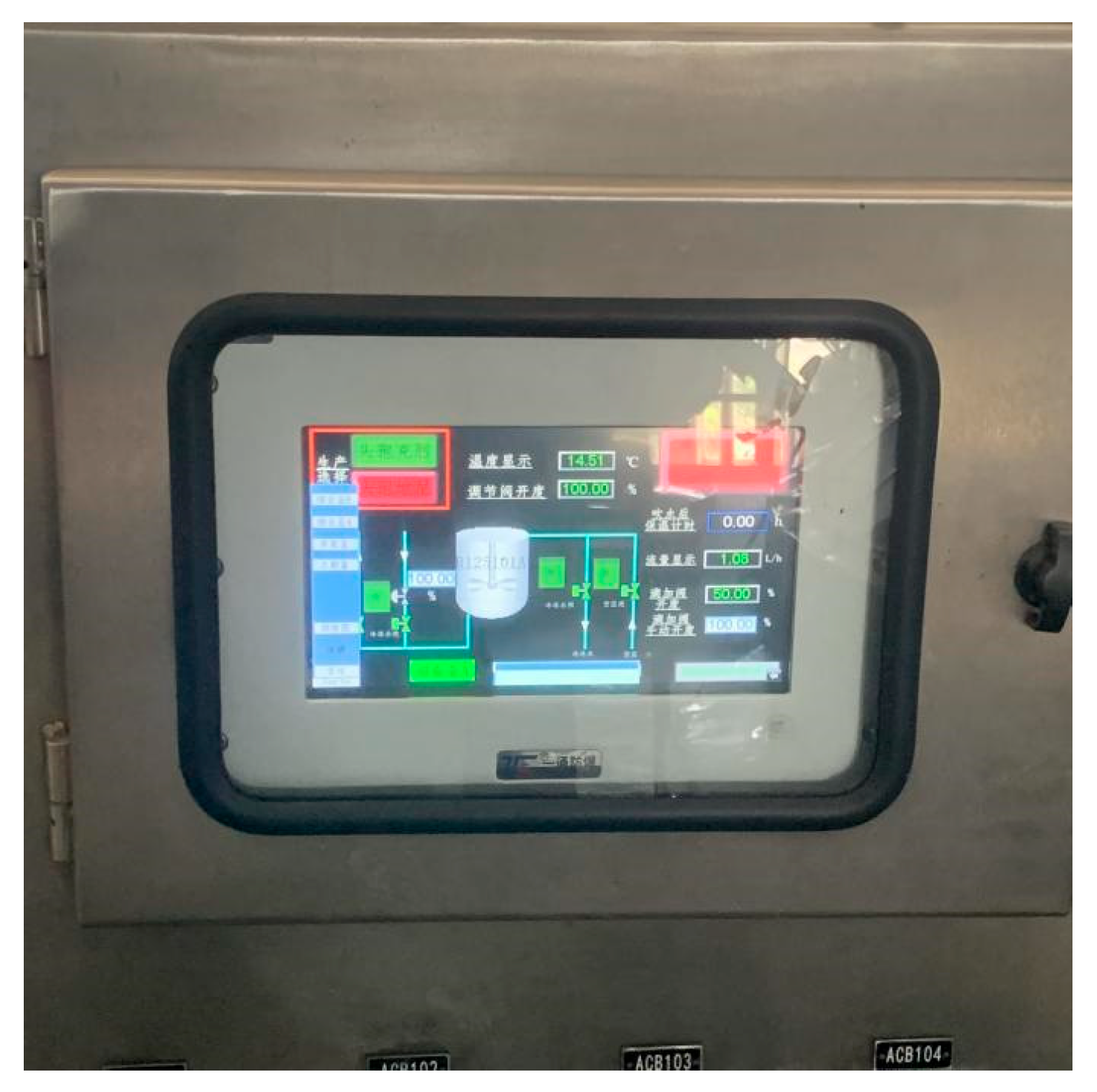
3.1. Selection of Data

The temperature data of a chemical company in Hengdian, Zhejiang Province, China, is used as the usual production reaction temperature of the reactor in this research. Figure 6 shows the trend of temperature data. A total of 400 sets of real-time temperature data of the reactor’s normal production are gathered, with the first 300 sets utilized as training samples and the last 100 sets used as prediction samples. Figure 7 depicts the reactor of the enterprise site’s production reaction. The temperature data is formed from the temperature sensor in this kettle and sent to the control cabinet in Figure 8; the reactor’s internal temperature range is 7 to 30 degrees Celsius; the temperature data is collected from the control cabinet seen in Figure 8; and Table 1 displays the reactor temperature data. It can be seen from the trend that samples 0–100 are the temperature of the reactor when there is no charging at the beginning, samples 100–200 belong to the reaction heating stage of the material, and samples 200–400 belong to the stage when the material begins to release heat.

3.2. Indices for Performance Evaluation

This article uses Matlab2021a, and the CPU is an 11th Gen Intel(R) Core(TM) i5-11300 H @3.10 GHz, 11 GHz, RAM = 16 G. To assess the prediction accuracy and performance of various models in a more intuitive manner, this study examines the prediction efficacy of the models using the mean absolute error, root mean square error, and the coefficient of determination R2 as the evaluation indicators. The smaller the values of MAE and RMSE, the more effective the prediction model and the better the algorithm’s performance.
The specific formula for evaluation is as follows [29,30]:
(1)
MAE
M A E = 1 n i = 1 n o ^ i o i .
(2)
RMSE
R M S E = 1 n i = 1 n o ^ i o i 2
(3)
R 2
R 2 = i = 1 N T i O i 2 / i = 1 N O i O avg 2
Figure 9, Figure 10 and Figure 11 show a direct comparison of the predicted and measured temperatures of the reactor by the combined optimization models of various neural networks and CPSO-RBF-BP neural networks. It can be seen that the single BP neural network model has a significant deviation from the expected displacement trend. The expected change trend of the CPSO-RBF-BP neural network prediction model matched the measured value. The CPSO-RBF-BP model was the nearest to the measured value in a comparison of four combinatorial optimization models. Figure 12 and Figure 13 depict the network error shift and fitting curve of the CPSO-RBF-BP model during training. It can be seen that the CPSO-RBF-BP network model outperforms the BP, RBF-BP, and PSO-RBF-BP networks in terms of error efficiency. Only a few spots are outside the fitting curve, and the fitting coefficient is 0.9966. Table 2 provides a comparison of various predicted values. According to the experimental data, the BP error is big, the RBF-BP combined neural network error is moderate, and the CPSO-RBF-BP error is considerably lower than the other two types of prediction. Table 3 displays the mean absolute error, root means square error, and coefficient of determination of predicted reactor temperature values for various combination optimization models. The mean absolute error of the CPSO-RBF-BP model is 0.114, the root mean square error is 0.173, and the coefficient of determination is 0.9966. It has better prediction accuracy when compared to the other three prediction models, proving the model’s superiority and effectiveness. The experimental findings indicate that when compared to the BP, RBF-BP, and PSO-RBF-BP neural network models, the prediction model optimized by the RBF-BP neural network using the chaotic particle swarm optimization algorithm can better reflect the trend of reactor temperature and is more practicable.

4. Conclusions

(1)
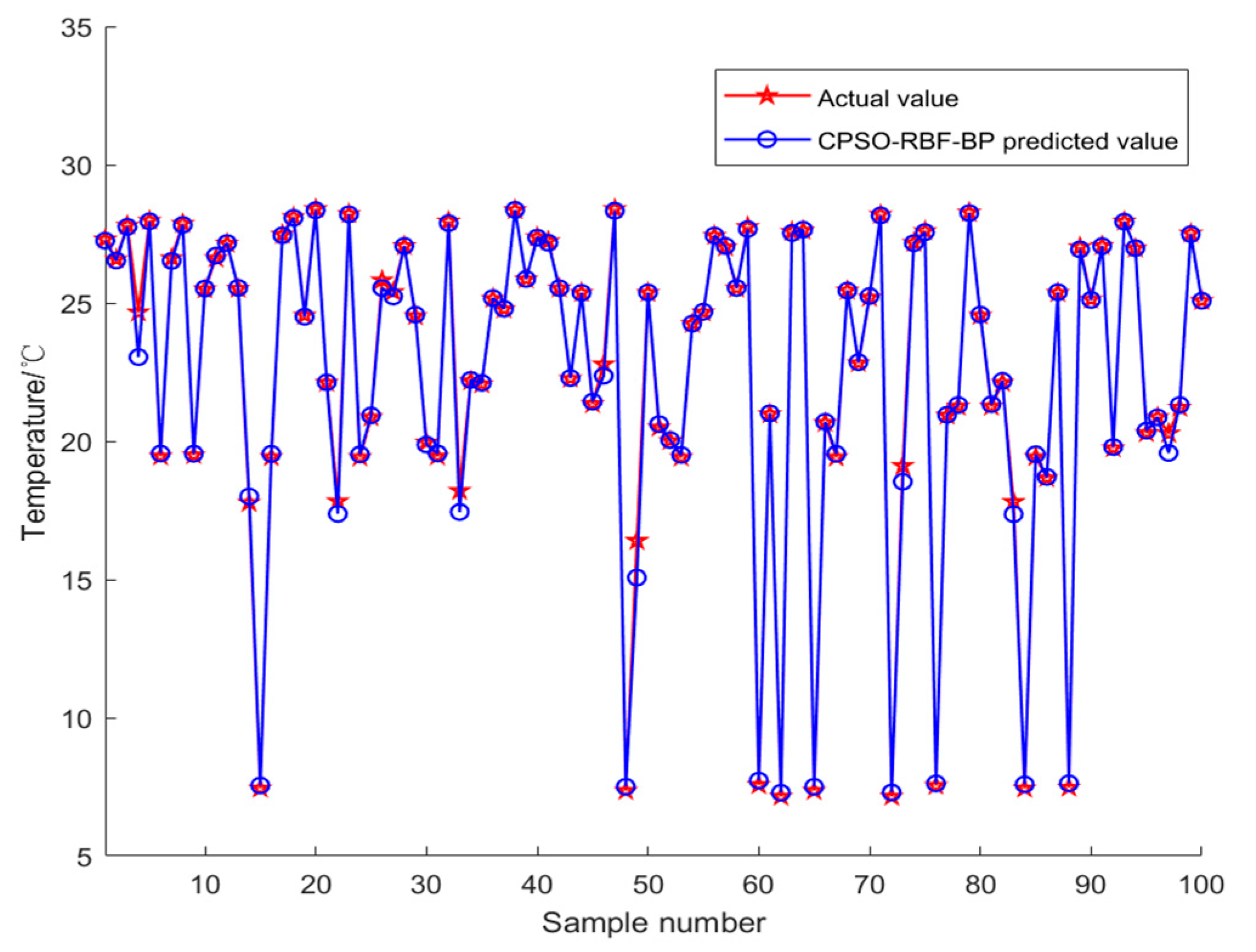
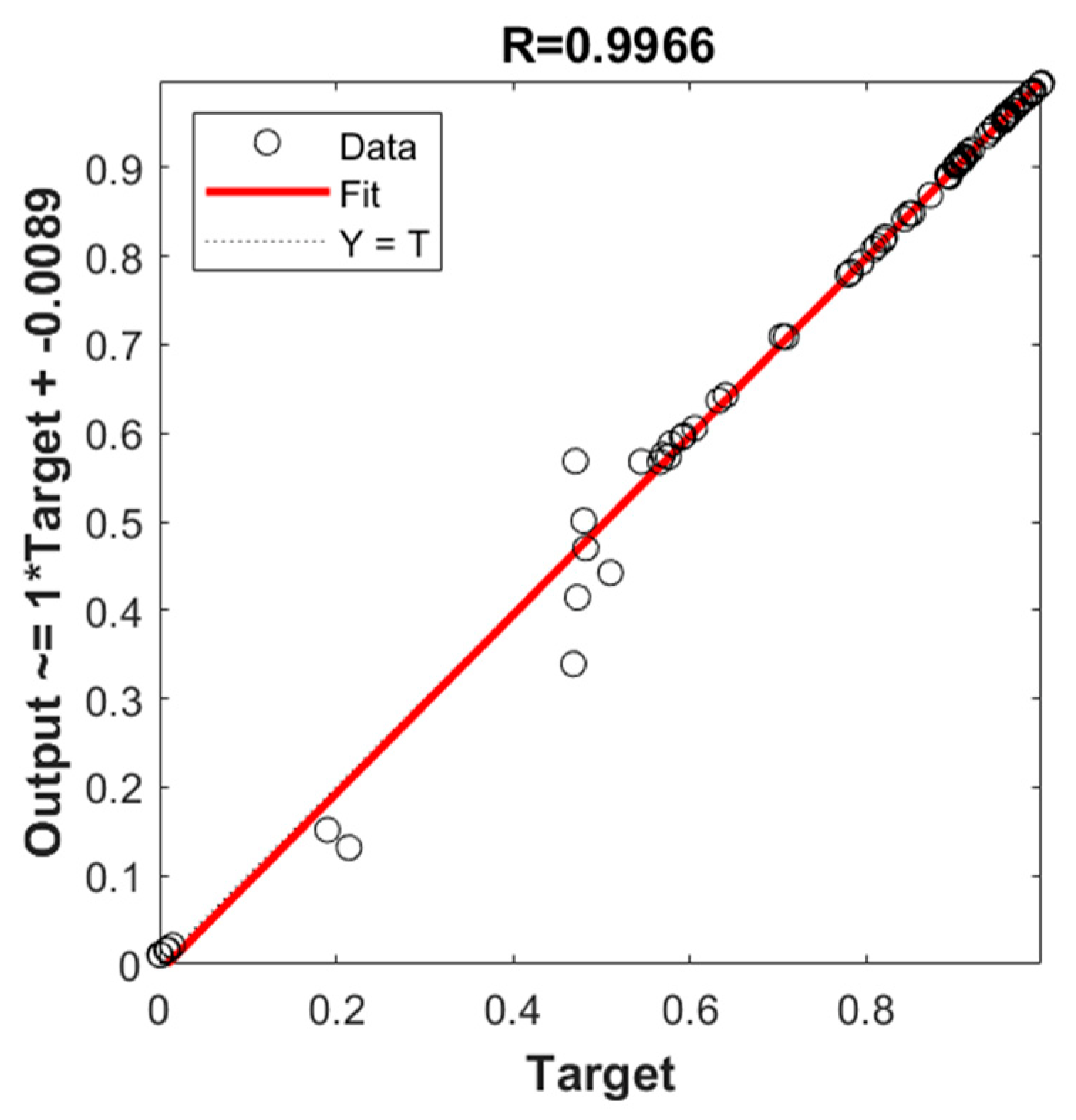
The control object in this study was the reactor of a chemical enterprise in Hengdian, Zhejiang, China. Because reactor temperature control is inaccurate, it is always a difficult issue for businesses to overcome. A chaotic particle algorithm CPSO is suggested in this paper to optimize the RBF-BP neural network model of the reactor temperature prediction control method. In this study, the CPSO optimization algorithm was used to correct the RBF-BP model’s weights and thresholds, and the impact of initial weight and threshold uncertainties on the training efficiency of the RBF-BP combined neural network was investigated. Other prediction models were used in this study for prediction comparison at the same time. Among several prediction datasets, the CPSO-RBF-BP model outperformed the BP and RBF-BP models in terms of prediction accuracy. The CPSO-RBF-BP variant is extremely accurate.
(2)
The simulation findings indicate that the proposed prediction method outperforms the BP and RBF-BP neural network prediction models in all aspects. The CPSO-RBF-BP mixed neural network model has a root mean square error of 17.3%, an average absolute error of 11.4%, and a fitting value of 99.791%. The CPSO-RBF-BP model used in this article outperforms the BP and RBF-BP neural network models in terms of control performance. The RBF-BP neural network model used in this paper has good nonlinear mapping ability, which accounts for better control performance. The optimal and suitable control variables can be found thanks to the chaotic particle swarm optimization CPSO algorithm’s good convergence and optimization ability. The optimum control variable for the reactor temperature can be used. The simulation results demonstrate the effectiveness of the proposed predictive control technique.
(3)
At the moment, only a subset of the data described in this article has been collected, which is all data from normal operation, and data from various factors affecting the temperature of the reactor is missing. Later, the operation data will be supplemented, and the prediction model for various temperature factors will be constructed to make the model universal, and the model will be applied to real production at the same time.

Author Contributions

Conceptualization, X.T. and Z.X.; methodology, X.T.; software, X.T.; validation, X.T. and B.X.; formal analysis, X.T. and Z.X.; investigation, X.T.; resources, X.T.; data curation, X.T.; writing—original draft preparation, X.T.; writing—review and editing, Z.X. and B.X.; visualization, X.T.; supervision, B.X.; project administration, B.X.; All authors have read and agreed to the published version of the manuscript.

Funding

This research received no external funding.

Institutional Review Board Statement

Not applicable.

Informed Consent Statement

Not applicable.

Data Availability Statement

Not applicable.

Conflicts of Interest

The authors declare no conflict of interest.

References

  1. Cervantes, A.L.; Agamennoni, O.E.; Figueroa, J.L. A nonlinear model predictive control system based on Wiener piecewise linear models. J. Process Control 2003, 13, 655–666. [Google Scholar] [CrossRef]
  2. Arefi, M.M.; Montazeria, A.; Poshtana, J.; Motlagh, M. Wiener neural identification and predictive control of a more realistic plug flow tubular reactor. Chem. Eng. J. 2007, 138, 274–282. [Google Scholar] [CrossRef]
  3. Venkateswarlu, C.; Rao, K.V. Dynamic recurrent radial basis model predictive control of unstable function network nonlinear process. Chem. Eng. Sci. 2005, 60, 6718–6732. [Google Scholar] [CrossRef]
  4. Bao, Z.; Pi, D.; Sun, Y. Nonlinear Model Predictive Control Based on Support Vector Machine with Multi-kernel. Chin. J. Chem. Eng. 2007, 15, 691–697. [Google Scholar] [CrossRef]
  5. Zhang, R.D.; Wang, S.Q. Support vector machine based predictive functional control design for output temperature of coking furnace. J. Process Control 2008, 18, 439–448. [Google Scholar] [CrossRef]
  6. Liu, C.; Ding, W.; Li, Z. Prediction of high-speed grinding temperature of titanium matrix composites using BP neural network based on PSO algorithm. Int. J. Adv. Manuf. Technol. 2016, 89, 2277–2285. [Google Scholar] [CrossRef]
  7. Liu, Y.; Lei, S.; Sun, C. A multivariate forecasting method for short-term load using chaotic features and RBF neural network. Eur. Trans. Electr. Power 2011, 21, 1376–1391. [Google Scholar] [CrossRef]
  8. Zhang, L.; Wang, T.; Liu, S.; Fang, K. Prediction model of PM2.5 concentration Based on CPSO-BP Neural Network. J. Gansu Sci. 2019, 32, 47–50+62. [Google Scholar]
  9. Yang, Q. Research on Predictive Control Method Based on CPSO-RBF Neural Network Algorithm. J. Guiyang Coll. (Nat. Sci. Ed.) 2021, 3, 13–17. [Google Scholar]
  10. Wu, X.; Mou, L. Research on Prediction Method Based on improved RBF-BP Neural Network. Foreign Electron. Meas. Technol. 2022, 9, 105–110. [Google Scholar]
  11. Li, Y.; Ding, J.; Sun, B.; Guan, S. Comparison of BP and RBF neural networks for short-term prediction of sea surface temperature and salinity. Adv. Mar. Sci. 2022, 40, 220–232. [Google Scholar]
  12. Zulqurnain, S.; Adi, A.; Sanaullah, D.; Muhammad, A.R.; Gilder, C.A.; Soheil, S.; Sadat, R.; Mohamed, R.A. A mathematical model of coronavirus transmission by using the heuristic computing neural networks. Eng. Anal. Bound. Elem. 2023, 146, 473–482. [Google Scholar]
  13. Zulqurnain, S.; Sadat, R.; Mohamed, R.A.; Salem, B.S.; Muhammad, A. A numerical performance of the novel fractional water pollution model through the Levenberg-Marquardt backpropagation method. Arab. J. Chem. 2023, 16, 104493. [Google Scholar]
  14. Mukdasai, K.; Sabir, Z.R.; Singkibud, P.; Sadat, R.; Ali, M. A computational supervised neural network procedure for the fractional SIQ mathematical model. Eur. Phys. J. Spec. Top. 2023, 1–12. [Google Scholar] [CrossRef]
  15. Latif, S.; Sabir, Z.; Raja, M.A.Z.; Altamirano, G.C.; Núñez, R.A.S.; Gago, D.O.; Sadat, R.; Ali, M.R. IoT technology enabled stochastic computing paradigm for numerical simulation of heterogeneous mosquito model. Multimed. Tools Appl. 2022. [Google Scholar] [CrossRef]
  16. Akkilic, A.N.; Sabir, Z.; Raja, A.M.Z.; Bulut, H.; Sadat, R.; Ali, M.R. Numerical performances through artificial neural networks for solving the vector-borne disease with lifelong immunity. Comput. Methods Biomech. Biomed. Eng. 2022. [Google Scholar] [CrossRef]
  17. Du, H.; Xie, G.-Z. GA-BP network algorithm based on optimization of mixed gas recognition. J. Electron. Compon. Mater. 2019, 38, 69–79. [Google Scholar]
  18. Wang, X.M.; Xu, J.P.; He, Y. Stress and Temperature Prediction of aero-Engine Compressor Disk Based on Multi-layer Perceptron. J. Air Power 2022, 1–9. [Google Scholar] [CrossRef]
  19. Wang, R.; Wang, Q.Q.; Lu, J. Short-term Load Forecasting Based on Stochastic Neural Network. Manuf. Autom. 2019, 41, 44–48. [Google Scholar]
  20. Panda, S.; Chakraborty, D.; Pal, S. Flank wear prediction in drilling using back propagation neural network and radial basis function network. Appl. Soft Comput. 2008, 8, 858–871. [Google Scholar] [CrossRef]
  21. Peng, G.; Nourani, M.; Harvey, J.; Dave, H. Feature selection using f-statistic values for EEG signal analysis. In Proceedings of the 42nd Annual International Conference of the IEEE Engineering in Biomedicine and Biology Society (EMBC), Montreal, QC, Canada, 20–24 July 2020; pp. 5936–5966. [Google Scholar]
  22. Zhang, X.L.; Li, J.H.; Li, J.X.; Wei, K.L.; Kang, X.N. Morphology defect identification based on Hybrid Optimization RBF-BP Network. Fuzzy Syst. Math. 2020, 34, 149–156. [Google Scholar]
  23. Yi, Z.M.; Deng, Z.D.; Qin, J.Z.; Liu, Q.; Du, D.; Zhang, D.S. Based on RBF and BP hybrid neural network of sintering flue gas NOx prediction. J. Iron Steel Res. 2020, 32, 639–646. [Google Scholar]
  24. Shankar, R.; Narayanan, G.; Robert, Č.; Rama, C.N.; Subham, P.; Kanak, K. Hybridized particle swarm—Gravitational search algorithm for process optimization. Processes 2022, 10, 616. [Google Scholar] [CrossRef]
  25. Kennedy, J.; Eberhart, R. Particle swarm optimization. In Proceedings of the ICNN’95—International Conference on Neural Networks, Perth, WA, Australia, 27 November–1 December 1995; Volume 4, pp. 1942–1948. [Google Scholar]
  26. Hefny, H.A.; Azab, S.S. Chaotic particle swarm optimization. In Proceedings of the 2010 the 7th International Conference on Informatics and Systems (INFOS), Cairo, Egypt, 28–30 March 2010; pp. 1–8. [Google Scholar]
  27. Sheng, X.; Zhu, W. Application of particle swarm optimization in soil simulation. Sci. Technol. Inf. 2012, 15, 90–92. [Google Scholar]
  28. Zeng, Y.Y.; Feng, Y.X.; Zhao, W.T. Adaptive Variable Scale Chaotic Particle Swarm Optimization Algorithm Based on logistic Mapping. J. Syst. Simul. 2017, 29, 2241–2246. [Google Scholar]
  29. Dey, K.; Kalita, K.; Chakraborty, S. Prediction performance analysis of neural network models for an electrical discharge turning process. Int. J. Interact. Des. Manuf. (IJIDeM) 2022, 1–19. [Google Scholar] [CrossRef]
  30. Kumar, M.; Lenka, Č.; Raja, M.; Allam, B.; Muniyandy, E. Evaluation of the Quality of Practical Teaching of Agricultural Higher Vocational Courses Based on BP Neural Network. Appl. Sci. 2023, 13, 1180. [Google Scholar] [CrossRef]
Figure 1. RBF neural network structure.
Applsci 13 03230 g001
Figure 2. BP neural network idea.
Applsci 13 03230 g002
Figure 3. RBF-BP hybrid neural network model structure.
Applsci 13 03230 g003
Figure 4. Chaotic particle swarm optimization algorithm steps.
Applsci 13 03230 g004
Figure 5. Specific model creation stages for the CPSO-RBF-BP.
Applsci 13 03230 g005
Figure 6. Temperature data trend diagram.
Applsci 13 03230 g006
Figure 7. Enterprise site reactor.
Applsci 13 03230 g007
Figure 8. Reactor configuration control cabinet.
Applsci 13 03230 g008
Figure 9. BP neural network model prediction result.
Applsci 13 03230 g009
Figure 10. RBF-BP neural network model.
Applsci 13 03230 g010
Figure 11. Prediction results of CPSO-RBF-BP neural network model.
Applsci 13 03230 g011
Figure 12. CPSO-RBF-BP neural network training error.
Applsci 13 03230 g012
Figure 13. CPSO-RBF-BP neural network fitted curve.
Applsci 13 03230 g013
Table 1. Reactor temperature data.
NumberTemperature/°CNumber Temperature/°CNumberTemperature/°CNumberTemperature/°C
17.0210111.7520120.6830123.81
27.0210211.8120221.9530224.16
37.0610311.8020324.6330324.18
47.0610411.7620424.7530424.22
57.0610511.6320524.6830524.25
67.1110611.4020625.5730624.23
77.1210711.4120725.5730724.28
287.2312814.3422818.3032827.38
297.2312915.6322918.4232927.43
307.2513015.6623018.5033027.47
317.2513115.9623118.9133127.55
327.2513216.2823219.4833227.58
337.2313316.9623319.6633327.60
347.2713417.4223419.8133427.67
357.2713517.4223520.0133527.63
10011.7120020.3030023.4740029.47
Table 2. Comparison of different predictive neural networks.
Sample NumberBP
Actual/Predicted/Error
RBF-BP
Actual/Predicted/Error
CPSO-RBF-BP
Actual/Predicted/Error
207.517.830.327.657.62−0.0321.9521.900.05
407.317.480.1725.2125.240.0326.0626.080.02
6018.7418.850.1118.9118.920.017.517.500.01
8024.6323.45−1.1824.6323.22−1.4124.6324.620.01
10018.4215.35−3.0721.9522.620.6725.5725.530.04
Table 3. Comparison of four neural network evaluation metrics.
Neural NetworkRMSER2MAE
BP2.3910.687790.628
RBF-BP0.5070.902450.433
CPSO-RBF-BP0.2630.997910.114
Disclaimer/Publisher’s Note: The statements, opinions and data contained in all publications are solely those of the individual author(s) and contributor(s) and not of MDPI and/or the editor(s). MDPI and/or the editor(s) disclaim responsibility for any injury to people or property resulting from any ideas, methods, instructions or products referred to in the content.

