A Novel Open-Closed-Loop Control Strategy for Quadrotor Trajectory Tracking on Real-Time Control and Acquisition Platform

Abstract

This paper presents a novel closed-loop control strategy that can be applied to quadrotor trajectory tracking to improve the control accuracy and stability. Inspired by intelligent creatures, the composite control strategy combines the open-loop mode and closed-loop control to overcome some disadvantages of oscillation and overshoot under feedback control mechanisms. The open-loop mode was realized by the quadrotor maneuverability model, which is proposed to build the bridge between the flight control commands and the desired acceleration. Then, a real-time control and acquisition platform with high-precision positioning, low-delay communication, and asynchronous distribution was built to collect the UAV’s real-time flight trajectory data for training the maneuverability model and to control the quadrotors asynchronously. Based on the platform and the trained model, the composite control mode on the closed-loop of the Proportional–Integral–Derivative (PID) control and the open-loop of the Long Short-Term Memory (LSTM) maneuverability model was implemented and verified. The experimental results show that the open-loop control strategy has a better advantage in the unity of time and space over the existing techniques for improving the UAV dynamic obstacle avoidance capability.

1. Introduction

Unmanned Aerial Vehicles (UAVs) have shown great potential in aerial photography, plant protection, disaster relief, route inspection, and other fields [1,2,3,4]. Compared with helicopters, UAVs have a better flexibility, simpler mechanical structure, and stronger maneuverability. However, the common quadrotor UAV is a typical nonlinear and dynamically unstable system, and the trajectory tracking is easily affected by internal uncertainties from the control model and external disturbances from the flight environment. Many nonlinear control methods have been implemented to solve these problems in space and time, such as back-stepping, sliding mode control, and a combination of them [5,6,7,8]. The back-stepping method can enhance the adaptability and robustness of the quadrotor system, but it has the problem of over-parameterization with an increase in the instructions [9,10,11]. Then, the sliding mode controller in the outer loop position subsystem was developed to ensure a robust tracking performance, even under the internal uncertainty and external disturbance of the time-varying control mode [12]. However, there is a serious chattering tendency in the presence of unmodeled actuator dynamics. Therefore, their hybrid control techniques were proposed to ensure the accuracy of trajectory tracking in the case of disturbance and to improve the system stability using the Lyapunov stability analysis. The above closed-loop and nonlinear control methods work well, and they greatly reduce the control cost in practical UAV applications. However, they have the common defects of oscillation and the overshoot phenomenon, which reduce the accuracy of trajectory tracking, and long-time overshoot will cause serious problems to the physical system.

To address these shortcomings, some researchers have also used neural networks to learn the quadrotor dynamics via offline or online means because neural networks have superior capabilities of self-learning and high-efficiency optimal solutions [13,14,15]. A novel nonlinear controller using neural networks and output feedback was implemented to learn the complete dynamic characteristic of the control system, including uncertain nonlinear terms such as aerodynamic friction and blade flapping [16]. An iterative learning algorithm that exploits the previous trajectory data was proposed to anticipate the recurrent disturbances of the system and proactively compensate for them. This approach is applied to quadrotor vehicles, and trajectory tracking can be achieved by a pure feedforward adaptation of the input signal [17]. However, these data-based control algorithms are still based on feedback control mechanisms and enhanced by reduplicative operating conditions and controlled environments.

According to the above questions, the trajectory implementation of intelligent creatures inspires us and offers a possible similar solution to overcome some drawbacks of oscillation and overshoot. Intelligent creatures train themselves many times in order to be familiar with the limits of their maneuverability in different states and make a feasible trajectory planning strategy in accordance with their capability. The biologically inspired heuristic method has also been used for UAVs or the swarm control strategy [18,19,20]. A novel tracking control strategy that integrates a bio-inspired back-stepping controller and a torque controller is presented. It takes into account system measurement noise and robot dynamic constraints, and avoids the shortcomings of large velocity jumps and overshoot problems in conventional back-stepping control [18]. A metaheuristic swarm coordination method of UAVs used in target search is based on flocking and stigmergy to provide robust formation control and dynamic environmental information sharing, respectively. The quality of the resulting cooperation is better in terms of swarm formation, search efficiency, strategy, and scalability [19].

Intelligent animals adopt a combination of open-loop and closed-loop control modes. This control method combines the simplicity and high-precision characteristics of open-loop control and the stability characteristics of closed-loop control. Then, the whole control process of stability, speed, and unity of time and space is realized. From these biological control mechanisms, a novel open-closed-loop control mode is proposed to try to solve the above problems of the feedback control method. To achieve open-closed-loop control, it is necessary to build a control and data acquisition platform to collect real-time UAV state data and continuously control the UAV. In terms of the UAV platform, many researchers have made many research contributions in various aspects [21,22]. However, the platform of this proposal needs to be improved in many aspects to obtain real-time control instructions and corresponding state data for offline training later. Then, the UAV maneuverability model, which establishes the relationship between control commands and desired accelerations, was built and trained. Because each UAV’s maneuverability model is known, the trajectory planning of each UAV can avoid the control boundary crossing problem, and the planned trajectory can be transformed into specific control instructions. Thus, this trajectory tracking strategy in open-loop control mode can improve the internal dynamic oscillation and overshoot problems, and the precise flight trajectory reproduction on the unity of time and space can be realized.

The main contributions of this paper mainly consist of two parts. Firstly, a real-time control and acquisition platform with high-precision positioning, low-delay communication, and asynchronous distribution was built to collect the UAV real-time flight data and control the quadrotors asynchronously. A high positioning accuracy of ±15 cm was realized with the support of the multi-sensor fusion technique, and the transmission delay of wireless communication was only 3.0∼3.5 ms by adopting a double-data-link structure. Secondly, a novel control strategy for quadrotor trajectory tracking is proposed. As the key part of the control strategy, the maneuverability model is presented to bridge between the control commands and the desired acceleration. Then, the combined control mode on the PID closed-loop and the open-loop on the LSTM maneuverability model was determined and verified. The experimental results show the good consistency between the preset and actual speeds of the UAV when the proposed control model is used. The hybrid control strategy, which combines the high-precision characteristics of open-loop control and the stability characteristics of closed-loop control, can effectively reduce the system oscillation and overshoot that often occur in closed-loop and nonlinear control methods.

The rest of this paper is organized as follows. Section 2 describes the method, which involves the compound control method, maneuverability model, and high dynamic platform. In Section 3, the results of the platform, model, and flight experiments are shown and estimated. Finally, Section 4 illustrates the conclusions.

2. Method

In the conventional tracking process, it is difficult for the quadrotor to unify space and time with a closed-loop control mechanism. The UAV controller evaluates its real-time position and/or state and then calculates the PID output values corresponding to the desired values at the next moment. This pattern results in an error between the desired and actual positions. The error is then sent to the input of the closed-loop controller, and the new output values are used to force the UAVs to approach the target. Although the closed-loop control method guarantees a high spatial precision, the feedback mode makes it difficult to reach the target in a given time. To make the best of the biological and open-loop control mechanisms, position control cannot be used, and a one-to-one relationship should be established between the control commands and the desired acceleration under different situations. According to Newtonian mechanics and UAV PID control equations, a set of dynamic equations of the quadrotor trajectory can be generally expressed as

$$\left\{\begin{array}{c}\overrightarrow{P}\left(t\right)={\overrightarrow{P}}_0+{\int }_0^t{\overrightarrow{v}}_{0}dt+{\int }_0^t{\int }_0^t\overrightarrow{a}\left(t\right)dtdt\hfill \\ \overrightarrow{a}\left(t\right)=f\left(s,m,\overrightarrow{u}\left(t\right),\overrightarrow{v},V_{\mathrm{bat}},\cdots \cdots \right)\hfill \\ \overrightarrow{u}\left(t\right)=k_p\overrightarrow{e}\left(t\right)+k_i{\int }_0^t\overrightarrow{e}\left(t\right)dt+k_d\frac{d\overrightarrow{e}\left(t\right)}{dt}\hfill \\ \overrightarrow{e}\left(t\right)={\overrightarrow{\theta }}_{\mathit{desired}}-{\overrightarrow{\theta }}_{\mathit{actual}}\mathrm{or}{\overrightarrow{\omega }}_{\mathit{desired}}-{\overrightarrow{\omega }}_{\mathit{actual}}\hfill \\ {\overrightarrow{\theta }}_{\mathit{desired}}=g\left({\overrightarrow{Q}}_{\mathit{cont}}\right)\hfill \end{array}\right.$$

(1)

where $\overrightarrow{P}\left(t\right)$ represents the quadrotor position from the initial point, $\overrightarrow{u}\left(t\right)$ is the PID control output, $\overrightarrow{e}\left(t\right)$ is the angle error or angular velocity error, ${\overrightarrow{\theta }}_{desired}$ is the desired UAV angle, and ${\overrightarrow{Q}}_{cont}$ is the control commands. $\overrightarrow{a}\left(t\right)$ represents the actual acceleration under different conditions of the UAV structure (s), UAV weight (m), PID controller output ($\overrightarrow{u}\left(t\right)$), velocity ($\overrightarrow{v}$), battery voltage, etc. The $\overrightarrow{a}\left(t\right)$ function (f) is very complicated and changes over time; thus, it cannot be expressed as a calculus formula. From Formula (1), $\overrightarrow{a}\left(t\right)$ comes from ${\overrightarrow{Q}}_{cont}$ and the current state of the UAV. Then, $\overrightarrow{a}\left(t\right)$ can be expressed as

$$\overrightarrow{a}\left(t\right)=M(s,m,{\overrightarrow{Q}}_{cont},\overrightarrow{v},V_{bat},\dots \dots )$$

(2)

then

$${\overrightarrow{Q}}_{cont}=M^{-1}(s,m,\overrightarrow{a}{\left(t\right)}_{desired},\overrightarrow{v},V_{bat},\dots \dots )$$

(3)

The ${\overrightarrow{Q}}_{cont}$ function ($M^{-1}$) is defined as the maneuverability model that represents the relationship between ${\overrightarrow{Q}}_{cont}$ and $\overrightarrow{a}{\left(t\right)}_{desired}$ under the current UAV conditions (velocity, power, mechanical structure, etc.).

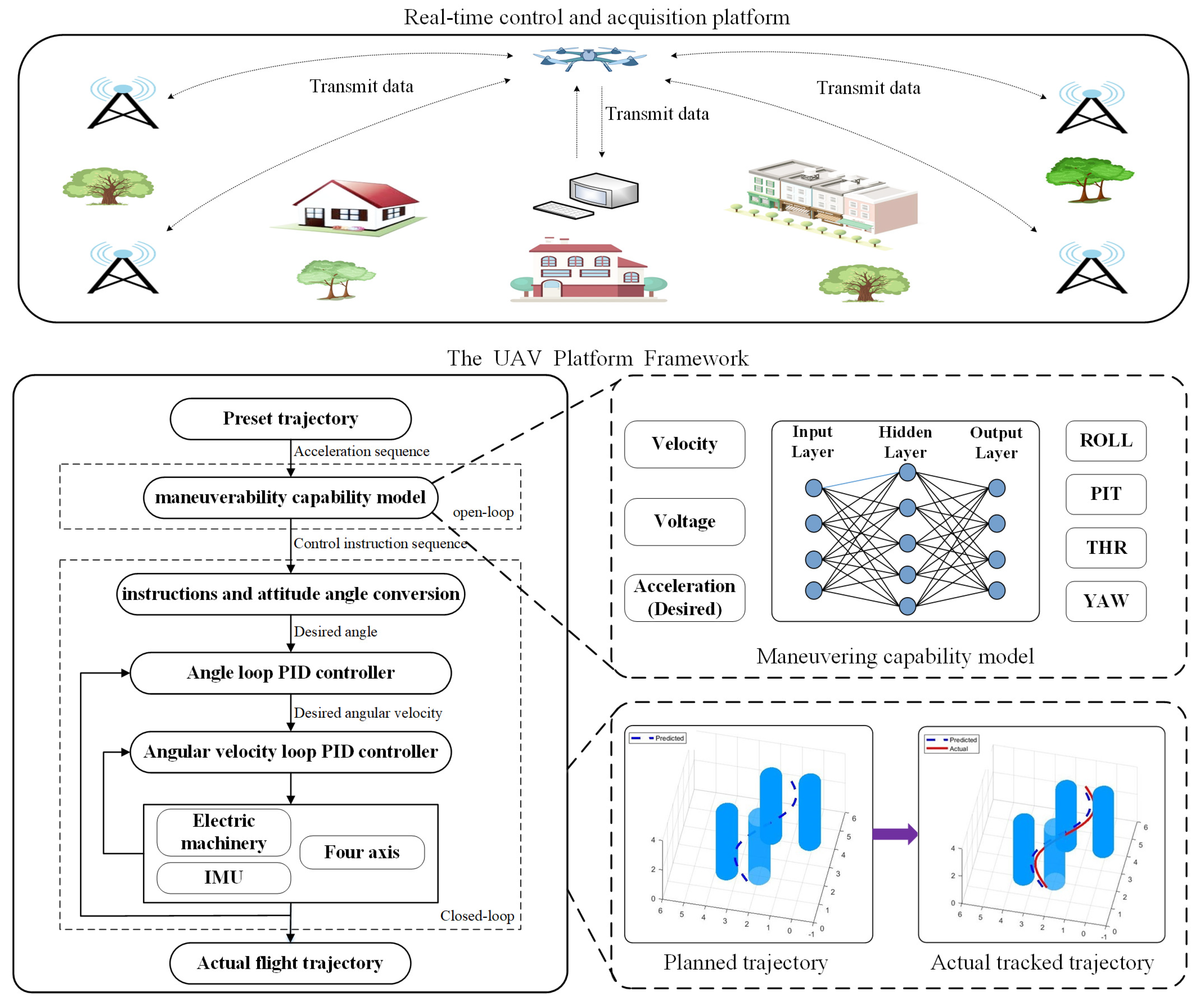
To implement this control method, a new open-closed-loop compound control strategy for trajectory tracking based on the proposed real-time platform is shown in Figure 1. The compound control strategy consists of three parts: a desired acceleration sequence generator, a maneuverability model, and a closed-loop controller. The maneuverability model was built from the data acquired by the real-time control and acquisition platform. The desired acceleration vector is the input of the maneuverability model, and the UAV control instructions are the output of the model.

The maneuverability model considers the control instructions and the current UAV states (speed, power, mechanical structure, etc.) as the influencing factors of the acceleration, and is trained many times from the actual flight data. As a result, a one-to-one relationship is obtained between the control instructions and the desired acceleration under different situations. This method can reproduce acceleration sequences that satisfy the spatial and temporal requirements of the given trajectory. The architecture of the control strategy is divided into three parts. Firstly, the preset trajectory generator needs to generate an optimal trajectory for reaching the target point, but this trajectory is generally an ideal acceleration sequence that has no correlation with the actual UAV. Secondly, the planned acceleration sequences need to be converted into actual control instructions. Due to the differences in the individual maneuverability of each UAV, it is necessary to build a maneuverability model containing the main state of each UAV and convert the expected acceleration sequence into an actual control instruction. Finally, the actual flight trajectory is implemented by a closed-loop control subsystem. As a bridge between desired accelerations and control instructions, the maneuverability model is trained to fit the UAV situation more accurately, and the deviation between the actual trajectory and the theoretical trajectory will be smaller.

2.1. Real-Time Control and Acquisition Platform

In order to implement the open-closed-loop composite method and obtain the flight data for model training, a highly dynamic control and acquisition platform is required to collect the real-time flight data of the UAV. The variables of the collected data include the control instruction, 3D position, acceleration, and battery voltage. To ensure the accuracy and integrity of real-time data, this high-dynamic control and acquisition platform is very different from the existing UAV control platforms, especially in low-delay communication and real-time accurate positioning.

Common UAV positioning techniques include Global Positioning System (GPS), Ultra Wide Band (UWB), Bluetooth, and acoustic positioning. The accuracy of GPS is in meters, and the accuracy can be improved to decimeters or centimeters through Real-Time Kinematic (RTK) technology. However, the GPS positioning frequency is slow, and it cannot meet the low-delay positioning requirements for this platform. If the GPS positioning refresh frequency is 10 Hz and the UAV speed is 5 m/s, the returned deviation of the UAV position data may reach 0.5 m with a low refresh rate. The communication delay time of ZigBee, Long-Range Radio (LoRa), or Bluetooth usually ranges from tens of milliseconds to hundreds of milliseconds, and they also further increase the position deviation of the flying UAV. Therefore, the communication delay time of the platform must also be set below a certain value. According to the common flight scenes of UAV clusters, it is necessary to build a real-time control and acquisition platform with positioning accuracy ≤±15 cm, communication delay time ≤ 20 ms, UAV state refresh frequency ≥ 25 Hz, and the number of supported UAV ≥ 10. To solve the contradiction of the positioning accuracy and refresh frequency in the platform, the multi-sensor fusion technology (UWB, optical flow sensor, and barometer) was adopted. The platform also has the problem of data communication blocking between the UAVs and the ground base station. Therefore, the wireless communication structure of the double data link, the reconstruction of the UAV control system, and the multi-thread processing technology of the ground base station were adopted to improve the acquisition accuracy and data integrity of the flying UAVs.

Figure 2 shows the block diagram of the real-time control and acquisition platform. The functions of flight monitoring, trajectory planning, multi-thread remote control, and log backup were performed in the host computer of the platform. In the UAV terminal, the UAV flight data acquisition, wireless communication with the host computer, and flight control were implemented to realize the actual trajectory. After software optimization, the average wireless transmission delay (sent from the ground station to the UAVs or returned from the UAVs to the ground station) can reach less than 5 ms, the serial port output rate is up to 500 kbps, and the packet loss ratio is less than 1%. The transmission delay is much lower than that of LoRa, ZigBee, and Wi-Fi. The UAVs adopt the positioning method composed of the UWB, optical flow sensor, and barometer. At the same time, the four-base-station scheme is arranged in the UWB positioning subsystem. The positioning refresh frequency of each UWB sensor can reach 350 Hz in the state of a single UAV, satisfying the high refresh requirement of the UAV state. In the rectangular positioning area of 15 × 15 m${}^2$, the average deviation fluctuation in static positioning is less than ±3 cm. The distributed and heterogeneous structure was designed to ensure that the UAVs can execute the preset real-time control instructions and collect real-time flight data simultaneously.

2.2. Dataset Building

It is necessary to measure a variety of flights that reflect the UAV maneuverability in different directions on the established platform. In automatic practical flight, the fixed-height mode is often used, and the other modes (take-off, landing, oblique acceleration, etc.) are relatively scarce. Meanwhile, the UAV has the phenomenon of jitter and tilt in the process of take-off and landing, and thus the collected data are unstable and irregular. In order to clearly describe the collected UAV flight data of different control commands under the commonly used condition, the direction of the UAV nose was defined as the positive x-axis (0°), and the vertical direction of the UAV nose on the right was defined as the positive y-axis (90°). Then, the flight trajectories in the eight horizontal directions (0°, 45°, 90°, 135°, 180°, 225°, 270°, and 315°) were selected and the corresponding flight data were collected. The original flight data have problems of fluctuation and consistency, so the data must be pre-processed and standardized. UAV data contain a large amount of variable information, such as acceleration, velocity, battery voltage, and control command values, and are widely distributed. It is easy for the data discreteness and non-uniformity to cause the convergence problem during model training. Therefore, it is necessary to preprocess these mass data.

Firstly, the originally collected data were classified and the data that changed illogically during the flight were discarded. If a set of data has abnormal fluctuations (such as UWB data abnormality, communication errors, etc.), these data are discarded and a new set of data is collected and obtained. Secondly, the Gaussian filter was used to filter the trajectory data to ensure that the subsequent calculation of the UAV velocity is more accurate. Finally, data standardization was performed after data preprocessing. Before the model training, the data standardization takes into account the weight initialization, which makes the data calculation easier in the initial training stage. After the model training, the output of the actual constructed algorithm model should be converted to the normalized values, and then the corresponding control instructions are obtained [23]. After Z-SCORE standardization of the flight data, the data conform to the standard normal distribution. The mean is 0 and the standard deviation is 1. This standardized method can play an important role when the data distribution is uneven and the situation is not clear. The conversion formula can be expressed as

$$Y\left(x\right)=\frac{x-\overline{x}}{\sigma }$$

(4)

where x is the initial value, $\overline{x}$ is the average value of all of the elements, and $\sigma$ is the standard deviation of all of the elements.

After the original data were selected, filtered, and standardized, a relatively complete flight database was formed. The database contains the data in eight flight directions, and tens of thousands of pieces were obtained as the dataset for the maneuverability model. Each piece of data contains five state variables (x-axis acceleration, y-axis acceleration, x-axis velocity, y-axis velocity, and battery voltage) and four control variables, which include the left–right control instruction (ROLL), the front–rear control instruction (PIT), the spin control instruction (YAW), and the throttle control instruction (THR).

2.3. Maneuverability Model

The maneuverability model is a regression model that aims to build a bridge between the desired acceleration and the control instructions while taking into account the influences of the UAV’s current state and external environmental factors. The higher the speed, the greater the drag on the UAV. Acceleration has a non-linear relationship with velocity influence. Due to an insufficient energy supply, the motor rotation speed will decrease under the same control instruction. Then, the input–output relationship of the maneuverability model on the constructed control platform was proposed to reflect the influence of these factors (Figure 1). Since the wind speed changes rapidly in the actual flight environment, it is difficult to obtain the relationship between UAV acceleration and fixed wind speed. The flight experiments were conducted under the condition of almost no wind, and the maneuverability model does not take wind speed into account. The input of the model includes the actual UAV velocity (including velocity in the x-direction and in the y-direction), the desired acceleration (including acceleration in the x-direction and in the y-direction), and the battery power supply. The output of the model is the control instructions, which include ROLL, PIT, YAW, and THR.

The regression prediction model is mainly divided into linear regression and nonlinear regression. In actual flight control, there is no linear relationship between UAV speed, power voltage, and air resistance. Then, a nonlinear regression model was adopted to build a bridge between the UAV state and instructions. At present, artificial neural networks (Back Propagation (BP), Recurrent Neural Networks (RNNs), etc.) are widely used to solve the nonlinear regression problem. The BP or RNN model does not consider the temporal relationship between variables, or cannot satisfy the temporal and spatial consistency requirement of the maneuverability model. They can only fuse information in a shorter time window. Then, the LSTM model was proposed to optimize this problem. In the flight experiment of the UAV, the acceleration is easily affected by the environment, and the information in one period will affect the flight state of the UAV. Based on the current situation and acceleration requirements, the output of the model (the desired instructions) depends on the period of the information segments; thus, RNN-LSTM was selected. The purpose of the RNN-LSTM model is to better store and retrieve previous information and to better extract long-distance dependencies with the data to improve the shortcomings of the RNN model.

The key idea of RNN-LSTM is that the final training result is obtained by combining LSTM memory cells. The LSTM maintains an uninterrupted error flow through the input and feedback, avoiding the long stagnation that forms among them. It can avoid the problem of gradient diffusion and gradient explosion. The LSTM units can store information for long periods of time and exploit long-distance dependencies in the data. The access to this memory unit is controlled by some special logical unit doors, which contain the functions of data storage, writing, and reading. These logic units are required to implement the correct value for each gate and select the gate function by different permissions. The flow chart of the UAV maneuverability model on the RNN-LSTM algorithm is shown in Figure 3. In the input layer, the input data sequences of the UAV, which are the voltage, velocity, and acceleration of the UAV during the flight, are defined. There are five layers in the hidden layer. $h_{n-1}$ and $c_{n-1}$ are the output and state of the middle LSTM memory cell, respectively. In the training layer, the actual loss function value is calculated according to the theoretical output and the model output, and then continuously fed back to the hidden layer. The loss function used is the root mean square (RMS) error function. Finally, after the prediction was made on the actual output results, batch normalization and de-normalization of the data were performed to obtain the actual prediction results.

3. Results

3.1. Platform Performance

The communication delay and positioning on the real-time platform must be evaluated as accurately as possible because they are directly related to the accuracy of the maneuverability model. After the functional testing of the platform, the measurement environment depended on the control ground station, and the UAV debugging mode was set up. For the wireless transmission delay, the half delay time of the wireless data sent from the ground station to the UAV and then returned from the UAV to the ground station was defined as the wireless signal transmission delay. The sets of MAVLink heartbeat packets were sent to the UAV and returned, and the average transmission delay value was only 3.0∼3.5 ms from the statistical data in the test environment of different transmission rates.

The measurement of positioning accuracy requires selecting nine positions and acquiring the corresponding coordinate values many times with the UWB positioning subsystem of four base stations. An optical flow sensor and barometer were used to ensure the redundancy and stability of the system. If obvious fluctuations or errors appear in the UWB positioning values, the data obtained from other positioning methods were used to modify and supplement. The positioning accuracy of the static UAV mode was obtained through multiple tests at the detection point, and the RMS errors of the results were analyzed. To further obtain the positioning accuracy of the UAV in dynamic mode, the UAV was controlled to hover in the position under the remote control state. Figure 4 shows the data collected with the UAV hovering in the position (3.000, 3.000, 1.000). The position fluctuation is within 15 cm. Influenced by the drift of the UAV while hovering, the coordinate values in Figure 4a will also drift in the horizontal direction to some extent. In the height direction, the results show that the error is still within 15 cm.

3.2. Dataset Built From Platform

When all functions (flight control, data acquisition, interactive interface, etc.) and the performance of the high-dynamic platform met the preset requirements, a typical UAV type-550 was selected and flight data acquisition was performed under different conditions. Figure 5 shows the actual scene of the UAV flight, which consists of a UAV, four UWB ground stations, and the host computer. The height of each UWB receiver was set to 1.8 m, and the square field size of four UWB receivers was 15 × 15 m${}^2$.

The UAV flight data were collected in manual remote control mode. The flight measurements were performed in different directions, and the corresponding flight data were collected with different remote control instructions. The acceleration, velocity, and battery voltage were changed in real-time as the UAV control instructions increased. Due to the fluctuation in the measured trajectory by the UWB, the relatively accurate real-time velocity was obtained by trajectory derivation after Gaussian filtering. The test showed that the response time of the UAV after receiving the control instructions is less than 30 ms, so the sampling interval of the UAV flight data was set to 40 ms. After the data pre-processing, the data table between the UAV control instruction, acceleration, velocity, and battery voltage was obtained. Figure 6 shows a set of real-time flight data with a type-550 UAV in a 90° direction in manual remote control mode. The total experimental dataset includes 12,800 pieces of flight records in eight directions. The x-axis in Figure 6a–d indicate the sampling time in seconds. As shown in Figure 6a,d, the acceleration and control values of the UAV are in the manual remote control mode. The ROLL control value is changed and the other three variables (PIT, YAW, and THR) are all set to 1500 in Figure 6d. Both the speed of the UAV and the battery voltage show a steady rate of change, which is shown in Figure 6b,c. In the subsequent experiments, we found that the maximum acceleration of the UAV reduced as the battery voltage decreased when the UAV was flying with the maximum control value. Thus, it can be determined that different battery voltages will affect the control state of the UAV at the same control command.

3.3. Verification of Maneuverability Model

To evaluate the regression prediction ability of the RNN-LSTM model, the RNN-LSTM and BP models were trained synchronously using the above dataset. In the proposed RNN-LSTM model, the five input nodes contain the actual acceleration ($Ac{c}_x$ and $Ac{c}_y$), velocity ($v_x$ and $v_y$), and power information of the UAV. Each hidden layer (five layers in total) uses 256 memory units and uses ReLU as the activation function. The output layer consists of four neurons that are activated using the ReLU function to output the four control variables of the UAV. In addition, the timestep parameter in the RNN-LSTM network was set to 6. During model training, the Root Mean Square Error (RMSE) loss function was optimized for the regression task. The Adaptive Moment Estimation (Adam) implementation of gradient descent was used to optimize the weights, and the initial learning rate of Adam was $7\times {10}^{-6}$. Out of a total of 12,800 flight datasets, 10,240 flight data sets were used for model training, with a sample batch size of 320 and a total iteration count of 500, while 20% of the data collected during the last flight in each direction were used as the actual test dataset. Figure 7 shows the comparison of the actual instruction values of the UAV and the predicted instruction values of the RNN-LSTM model in eight different directions with the next 32 consecutive time points. For the UAV flight, the flight mode was set to a fixed altitude, the variables THR and YAW were kept at the median value of 1500, and the variables PIT and ROLL were mainly changed. To further compare the accuracy of different models,

Table 1. The errors of the BP and RNN-LSTM models in different directions.

Variable	Root Mean Square (LSTM (BP))
	ROLL	PIT	THR	YAW
0°	1.39 (3.91)	1.94 (4.42)	0.51 (0.51)	0.33 (0.34)
45°	2.62 (5.66)	2.21 (5.24)	1.81 (1.71)	0.94 (0.98)
90°	1.91 (7.22)	3.42 (6.45)	0.42 (0.41)	0.70 (0.69)
135°	1.53 (6.32)	1.87 (8.86)	0.76 (0.84)	0.54 (0.53)
180°	2.28 (4.88)	1.94 (4.24)	0.67 (0.67)	0.55 (0.55)
225°	1.83 (4.71)	1.74 (3.11)	1.17 (1.15)	0.47 (0.49)
270°	2.14 (5.37)	3.00 (7.42)	0.25 (0.27)	0.30 (0.27)
315°	1.60 (3.76)	2.05 (5.34)	0.51 (0.46)	0.41 (0.40)

shows the RMS errors of the BP and RNN-LSTM models. Since the THR and YAW variables are almost unchanged in the fixed-height mode, the corresponding RMS errors are relatively close. The ROLL and PIT variables change a lot, but it can be seen that the RMS errors of the RNN-LSTM model are smaller than those of the BP model. Since the ROLL and PIT variables are directly related to the acceleration values, it can be speculated that the UAV can be controlled more accurately by the RNN-LSTM model.

3.4. Experiments of Quadrotor Trajectory Tracking

The UAV flight demonstration on the RNN-LSTM maneuverability model is important for verifying the accuracy of the synchronous control in time and space. Two different UAV flights were carried out. The planned trajectories were designed and converted into the corresponding sets of control instructions by the maneuverability model. Then, the sets of control instructions were used to control the UAV flight, and the corresponding actual flight data were collected. Later, the evaluation focused on the consistency of the actual real-time flight data (velocity, acceleration, position, and time) with the planned trajectory data.

The planned trajectory of the straight flight is a process in which the UAV linearly increases its acceleration from an actionless state and then linearly decreases to zero. Figure 8 shows the comparison of the variables between the actual flight and the planned straight flight trajectory. It can be seen that the actual acceleration, velocity, and coordinate values collected at each moment are basically the same as the planned trajectory.

According to the coordinate values of the actual flight obtained in Figure 8d, the speed at each moment is calculated by the change in coordinate points. Since the deviation in the UAV positioning is ±15 cm, the actual coordination curve of the UAV has fluctuated within a certain numerical range, which is shown in Figure 8c,d. Then, the velocity calculated by only two coordinate points fluctuates greatly. Therefore, a mean filter with a window size of 50 sample points (equal to 2 s) was used to smooth the coordinates. Figure 8b shows the curve of the calculated velocity varying with time by filtering. If the accelerations are not monotonically increasing or decreasing in high-speed conditions, the velocity in the window was averaged to a lower value. This is the reason for why the maximum velocity value is much smaller than the theoretical value at this moment of 3.84 s. The final velocity of the UAV in the experiment is around 0, which is basically consistent with the planned trajectory. Due to the error accumulation, the deviation between the actual flight coordinate position and the preset position is larger when the actual flight position is farther from the initial position. The deviation between the final flight distance of the experiment and the preset path is approximately 0.7 m, and its error is within 6%. Compared with other control algorithms, our proposed open–closed loop hybrid strategy not only reduces system oscillation and overshoot, but also shows better consistency between the preset and actual velocity [16,17,18].

The quadrilateral flight, which is made up of four continuous straight flights, was implemented to further evaluate the accuracy of the strategy. The essential status of the planned trajectory is that the flight perimeter is 48 m, the maximum acceleration is 2.4 m/s${}^2$, and the maximum velocity is 4.6 m/s. Figure 9 shows the coordinate curves of the actual flight trajectory on the maneuverability prediction model and the preset trajectory. It can be seen that the two flight trajectories maintain a good consistency during the time changes. Since the UAV tends to drift slightly after launch, it cannot be guaranteed to fly in the specified direction at the original point like the preset mode. To further analyze the accuracy of time and space control on the RNN-LSTM maneuverability model, the average speed and flight distance were counted by error degree. The average distance error per edge is approximately 1.0 m, which is still slightly far from control algorithms [5,6,9] that use the position error as the loss function. Since the proposed model takes the velocity and acceleration of the UAV as the input parameters of the model rather than the objective position information. The total flight error of the distance and speed on the maneuverability model is approximately 8% under the influence of uncertain environmental factors (low airspeed, air temperature, etc.). This means that the open-closed-loop compound control strategy is applicable for quadrotor trajectory tracking in order to realize the unification of time and space. The decision iteration time in actual UAV systems is much shorter than the flight time of a preset trajectory in the flight demonstrations. Therefore, if the fine-tuning mechanism is added to the control model and a more accurate model is established, the UAVs can be controlled more precisely in time and space.

4. Conclusions

This paper presents a novel open-loop control strategy for improving the control accuracy and stability of quadrotor trajectory tracking. The proposed strategy, which combines the high-precision characteristics of open-loop control and the stability characteristics of closed-loop control, can effectively reduce the system oscillation and overshoot existing in the current technology. Firstly, a real-time control and acquisition platform with high-precision positioning, low-delay communication, and asynchronous distribution was built to collect the UAV real-time flight trajectory data and control the quadrotors asynchronously. Secondly, the quadrotor maneuverability model was presented as the key part of the control strategy to bridge between the flight control instructions and the desired acceleration. Finally, the composite control mode on the RNN-LSTM maneuverability model was verified by an actual UAV flight demonstration. In the square flight task, the results show the effectiveness of the proposed hybrid control strategy on the unity of time and space. During the flight, the great consistency between the preset and actual values of the UAV control variables (including velocity and acceleration) was demonstrated to verify the superiority of the model. However, the total flight distance error is approximately 8% due to the lack of objective position information in the model. In future work, we will improve the model accuracy by adding more flight data, and then use more preset tracks of different shapes to demonstrate the robustness of our model.

References

1. Mademlis, I.; Mygdalis, V.; Nikolaidis, N.; Pitas, I. Challenges in Autonomous UAV Cinematography: An Overview. In Proceedings of the 2018 IEEE International Conference on Multimedia and Expo (ICME), San Diego, CA, USA, 23–27 July 2018. [Google Scholar]
2. Liu, J.; Xu, W.; Guo, B.; Zhou, G.; Zhu, H. Accurate Mapping Method for UAV Photogrammetry Without Ground Control Points in the Map Projection Frame. IEEE Trans. Geosci. Remote Sens. 2021, 59, 9673–9681. [Google Scholar] [CrossRef]
3. Tokekar, P.; Hook, J.V.; Mulla, D.; Isler, V. Sensor Planning for a Symbiotic UAV and UGV System for Precision Agriculture. IEEE Trans. Robot. 2016, 32, 1498–1511. [Google Scholar] [CrossRef]
4. Do-Duy, T.; Nguyen, L.; Duong, T.; Khosravirad, S.; Claussen, H. Joint Optimisation of Real-Time Deployment and Resource Allocation for UAV-Aided Disaster Emergency Communications. IEEE J. Sel. Areas Commun. 2021, 39, 3411–3424. [Google Scholar] [CrossRef]
5. Zuo, Z.; Mallikarjunan, S. L1 Adaptive Backstepping for Robust Trajectory Tracking of UAVs. IEEE Trans. Ind. Electron. 2017, 64, 2944–2954. [Google Scholar] [CrossRef]
6. Zhang, J.; Gu, D.; Deng, C.; Wen, B. Robust and Adaptive Backstepping Control for Hexacopter UAVs. IEEE Access 2019, 7, 163502–163514. [Google Scholar] [CrossRef]
7. Chen, F.; Jiang, R.; Zhang, K.; Jiang, B.; Tao, G. Robust Backstepping Sliding-Mode Control and Observer-Based Fault Estimation for a Quadrotor UAV. IEEE Trans. Ind. Electron. 2016, 63, 5044–5056. [Google Scholar] [CrossRef]
8. Reinoso, M.J.; Minchala, L.I.; Ortiz, P.; Astdillo, D.F.; Verdugo, D. Trajectory tracking of a quadrotor using sliding mode control. IEEE Lat. Am. Trans. 2016, 14, 2157–2166. [Google Scholar] [CrossRef] [Green Version]
9. Xu, L.; Ma, H.; Guo, D.; Xie, A.; Song, D. Backstepping Sliding-Mode and Cascade Active Disturbance Rejection Control for a Quadrotor UAV. IEEE ASME Trans. Mechatron. 2020, 25, 2743–2753. [Google Scholar] [CrossRef]
10. Bhatia, A.K.; Jiang, J.; Zhen, Z.; Ahmed, N.; Rohra, A. Projection Modification Based Robust Adaptive Backstepping Control for Multipurpose Quadcopter UAV. IEEE Access 2019, 7, 154121–154130. [Google Scholar] [CrossRef]
11. Azinheira, J.R.; Moutinho, A. Hover Control of an UAV With Backstepping Design Including Input Saturations. IEEE Trans. Control Syst. Technol. 2008, 16, 517–526. [Google Scholar] [CrossRef]
12. Xu, B.; Lu, X. An Online Adaptive Control Strategy for Trajectory Tracking of Quadrotors Based on Fuzzy Approximation and Robust Sliding Mode Algorithm. IEEE Access 2020, 8, 215327–215342. [Google Scholar] [CrossRef]
13. Shin, J.; Kim, H.J.; Kim, Y.; Dixon, W.E. Autonomous Flight of the Rotorcraft-Based UAV Using RISE Feedback and NN Feedforward Terms. IEEE Trans. Control Syst. Technol. 2012, 20, 1392–1399. [Google Scholar] [CrossRef] [Green Version]
14. Shiri, H.; Park, J.; Bennis, M. Remote UAV Online Path Planning via Neural Network-Based Opportunistic Control. IEEE Wirel. Commun. Lett. 2020, 9, 861–865. [Google Scholar] [CrossRef] [Green Version]
15. Nodland, D.; Zargarzadeh, H.; Jagannathan, S. Neural Network-Based Optimal Adaptive Output Feedback Control of a Helicopter UAV. IEEE Trans. Neural Netw. Learn. Syst. 2013, 24, 1061–1073. [Google Scholar] [CrossRef] [PubMed]
16. Dierks, T.; Jagannathan, S. Output Feedback Control of a Quadrotor UAV Using Neural Networks. IEEE Trans. Neural Netw. 2010, 21, 50–66. [Google Scholar] [CrossRef] [PubMed]
17. Schoellig, A.P.; Mueller, F.L.; D’Andrea, R. Optimization-based iterative learning for precise quadrocopter trajectory tracking. Auton. Robot. 2012, 33, 103–127. [Google Scholar] [CrossRef] [Green Version]
18. Xu, Z.; Yang, S.X.; Gadsden, S.A. Enhanced Bioinspired Backstepping Control for a Mobile Robot With Unscented Kalman Filter. IEEE Access 2020, 8, 125899–125908. [Google Scholar] [CrossRef]
19. Alfeo, A.L.; Cimino, M.; Vaglini, G. Enhancing biologically inspired swarm behavior: Metaheuristics to foster the optimization of UAVs coordination in target search. Comput. Oper. Res. 2019, 110, 34–47. [Google Scholar] [CrossRef]
20. Wu, Q.; Shen, X.; Jin, Y.; Chen, Z.; Li, S.; Khan, A.; Chen, D. Intelligent Beetle Antennae Search for UAV Sensing and Avoidance of Obstacles. Sensors 2019, 19, 1758. [Google Scholar] [CrossRef] [Green Version]
21. Shao, G.; Ma, Y.; Malekian, R.; Yan, X.; Li, Z. A Novel Cooperative Platform Design for Coupled USV-UAV Systems. IEEE Trans. Ind. Inf. 2019, 15, 4913–4922. [Google Scholar] [CrossRef] [Green Version]
22. Ding, C.; Lu, L.; Wang, C.; Ding, C. Design, Sensing, and Control of a Novel UAV Platform for Aerial Drilling and Screwing. IEEE Robot. Autom. Lett. 2021, 6, 3176–3183. [Google Scholar] [CrossRef]
23. Birnbaum, Z.; Dolgikh, A.; Skormin, V.; O’Brien, E.; Muller, D.; Stracquodaine, C. Unmanned Aerial Vehicle Security Using Recursive Parameter Estimation. J. Intell. Robot Syst. 2016, 84, 107–120. [Google Scholar] [CrossRef]
Figure 1. Architecture of the open-closed-loop compound control strategy on the real-time control and acquisition platform.
Applsci 13 03251 g001
Figure 2. Block diagram of the real-time control and acquisition system.
Applsci 13 03251 g002
Figure 3. Flow chart of the RNN-LSTM maneuverability model.
Applsci 13 03251 g003
Figure 4. The positioning statistics of the UAV hovering in fixed position: (a) x-axis and y-axis position; and (b) z-axis position.
Applsci 13 03251 g004
Figure 5. The actual scene of UAV flight with a typical type-550.
Applsci 13 03251 g005
Figure 6. A set of the real-time flight data varies with the time at the 90° direction: (a) acceleration; (b) voltage; (c) velocity; and (d) control value.
Applsci 13 03251 g006
Figure 7. The contrast values of the RNN-LSTM prediction and the actual flight in different directions: (a) the x-axis positive direction; (b) the y-axis negative direction; (c) the x-axis positive and y-axis negative direction; and (d) the x-axis negative and y-axis positive direction.
Applsci 13 03251 g007
Figure 8. The contrast data between the actual flight and the preset trajectory in straight flight: (a) acceleration; (b) velocity; (c) y-axis position; and (d) x-axis position.
Applsci 13 03251 g008
Figure 9. Coordinate curves of the actual flight and preset trajectories.
Applsci 13 03251 g009