Abstract
Since machine learning is applied in medicine, more and more medical data for prediction has been produced by monitoring patients, such as symptoms information of diabetes. This paper establishes a frame called the Diabetes Medication Bayes Matrix (DTBM) to structure the relationship between the symptoms of diabetes and the medication regimens for machine learning. The eigenvector of the DTBM is the stable distribution of different symptoms and medication regimens. Based on the DTBM, this paper proposes a machine-learning algorithm for completing missing medical data, which provides a theoretical basis for the prediction of a Bayesian matrix with missing medical information. The experimental results show the rationality and applicability of the given algorithms.
1. Introduction
In daily life, the doctor judges the patient’s disease according to the symptoms monitoring and then formulates a medication plan for the patient based on the curative effect of different medication regimens. However, this process is mainly based on the statistical data of past cases [1,2,3]. The accuracy of the medication regimen directly affects the development of the patient’s condition and is the most critical link in the treatment process, while due to the diversity of diabetes complications and the diversity of diabetes-related drugs, the statistics from clinical tests often include missing values [4,5,6]. Completing these missing values based on the rules of the datasets can greatly enhance the accuracy of doctors’ judgments. The research on missing value completion in the existing literature mainly focuses on the low-rank matrix completion methods: Trever Hastie et al. applied low-rank SVD to advance the current matrix completion algorithms and developed a new algorithm that can deal with the Netflix competition data [7]. Gerome Vivar et al. used matrix completion to provide full data available for Computer Aided Diagnosis using machine learning [8]. Chen et al. proposed a Matrix Completion for Planning Diabetes Treatment by using nonlinear convex optimization to generate information [9]. Bhattacharya proposed two new estimators, based on singular value threshold and nuclear norm minimization, to recover the sparse matrix under this assumption [10]. However, in medical cases, the causal relationship between different symptoms and multiple medication regimens forms a full-rank Bayesian matrix, so the previous low-rank matrix completion methods are no longer applicable. Therefore, this paper develops a different matrix completion algorithm assuming the matrix has a full rank to provide better support for the choice of diabetes medication plan. This article establishes a method to complete a probabilities matrix by one eigenvector. Through actual case statistics, we find that it is easier to obtain the eigenvector with the DTBM eigenvalue of 1, that is, the probability of different symptoms in diabetic patients and the probability of each medication regimen being used. The data is obtained from medical tests after decades of sample statistics, which are the stable probability distributions of the symptoms and medication regimens in people with diabetes, and it mathematically conforms to the stable state theory of the Markov matrix. Based on the above information, we give the matrix completion algorithm for the DTBM, which accurately completes the 56 missing values by one eigenvector in Section 6. At the same time, the 56 completed values can be fixed into the two blocks of the DTBM, one block is the probabilities of medications given multiple symptoms, and another is the probabilities of symptoms given medications.
The new algorithm can complete an empty matrix from one eigenvector which can help doctors make a medication plan with limited information. This original work completes a DTBM with 56 missing data representing relations between symptoms and medications to support doctors making medical plans. The remainder of this article is organized as follows. In the second Section, this paper will introduce and explain two types of sample data about diabetic symptoms and regimens. Also, the article mentions the collecting and processing of these two kinds of sample data that are separated into causes and effects in one matrix. Section 3 will analyze the properties of the principle eigenvector of the DTBM for computing missing data in the sample data. Section 4 will demonstrate the method for completing missing data of one column in the DTBM using the principal eigenvector of the DTBM. In Section 5, an optimization algorithm is presented to deal with the situation that all the sample data is missed, and the eigenvector is the only information we know; Section 6 uses the proposed algorithms to complete an empty matrix about diabetes with 56 missing sample data; Section 7 discusses what the results we obtained in Section 6 mean and the differences between existed matrix completion methods and the method we proposed; Section 8 summarizes the main contributions and inadequacies of this paper.
2. Sample Data and Bayesian Matrix
In the case data of diabetes [11], we mainly analyze the relationship between symptoms and medication. Assume that the medication regimens are written as T = (t1, t2, …, tm), and the symptoms are written as S = (s1, s2, …, sn). We write the two sets of events in a comparison matrix:
Matrix B uses posterior probability (given the symptom, the probability of using different medications) and likelihood estimates (given the medication and the curative effect to different symptoms) to describe the relationship between symptoms and medications completely, which we call the Diabetes Medication Bayes Matrix (DTBM). The DTBM is a block matrix that contains four parts, among which the elements are represented by , q = 1, 2, 3, 4. represents the Probability of correlation between medication regimens, i = 1, 2, …, m, j = 1, 2, …, m. indicated the probability of different medication regimens received by patients with different symptoms. The elements in represent the effects of different medications on different symptoms in the case data, expressed by conditional probability, where i = m + 1, m + 2, …, m + n, j = 1, 2, …, m; represents the probability of correlation between different diseases, where i = m + 1, m + 2, …, m + n, j = m + 1, m + 2, …, m + n. Assuming that the medication regimens are independent and the symptoms of diabetic patients are independent. Therefore, .
The DTBM fully demonstrates how should diabetic patients with certain symptoms choose medication regimens. Doctors can also directly recommend medication regimens for patients based on the probability in . However, in the actual sampling and statistics process, due to the diversity and complexity of patient symptoms, there will be one or more missing columns. Currently, we need to do the completion.
3. The Eigenvector of the DTBM
Since indicates the conditional probability value, each element in the DTBM is between [0, 1]. And when a certain condition is given, the sum of its conditional probabilities is equal to 1. Therefore, the sum of each column in the DTBM is 1, which means that the DTBM is a Markov matrix. According to the characteristics of the Markov matrix, the DTBM has a principle eigenvector whose eigenvalue is equal to 1. So, what is this eigenvector?
The “0” in the matrix represents that there is no correlation between the occurrence of independent events set , which is consistent with Bayes’ theorem’s assumption. At this time, the probability of the presence of under events is expressed as , and the likelihood of the occurrence of under events set is shown as .
According to Bayes’ theorem and the formula of total probability, we get p(T), p(S).
Since P(X), P(Y), and are used to get , can be expressed by the eigenvalue equation:
It is not difficult to see that is the eigenvector of the DTBM when the eigenvalue equals 1. The eigenvector with an eigenvalue of 1 expresses a stable state of the DTBM. After decades of medication research and practice, diabetes complications can be treated with a certain drug, and the proportion of different drugs used for certain complications is stable. Meanwhile, in a relatively stable environment, the proportion of people with various diabetes symptoms also tends to stabilize. This eigenvector represents this stability, where p(t) and p(s) can be obtained through data statistics. Therefore, we need to find the missing column vectors in the DTBM based on its eigenvector.
4. DTBM Completion Algorithm for One Missing Column
We aim for a specific algorithm to fill in the missing value in the Diabetes medication Bayesian matrix when only the missing suggested proportion of each treatment plan under one specific symptom is missing (that is, when one column is missing). Since the eigenvector of the DTBM (Markov) matrix with an eigenvalue of 1 has m + n elements, we set the eigenvector as e, where the element is .
We can get Formula (1) according to the eigenvector’s property Be = 1e:
Assuming that the column r is null, then:
A certain missing value in can be obtained by Formula (3).
Or represented by the column vector of the matrix:
This model derives a matrix through its eigenvectors, and the elements in the matrix are the curative effects of different drug combinations on diabetic complications. The upper part of the eigenvector represents the probability of patients using a different medication (regimen) in the sample data, and the lower part represents the probability of patients having different indications in the sample data.
5. Missing Multiple Vectors
5.1. Only Missing Posterior Probability
In some real cases, there may be no statistics on the medications under multiple symptoms. In the second block of matrix B, not only one column could be missing, but multiple columns or even the entire block is empty. On the other hand, the likelihood estimate in the matrix is known and can be queried from existing research. Therefore, we can find each missing value according to Bayes’ theorem. Now taking two cases and two medication regimens as an example, the specific methods are as follows:
Assuming that B2 is unknown, we can get the elements in according to Bayes’ theorem:
5.2. Both the Posterior and the Likelihood Estimate Have Missing Values
In the cases when there is a great number of missing values in both and (for example, the case when only the possibility of the first drug used for each symptom is known, and other likelihood estimates and posterior probabilities are unknown.), To fill in the missing values, we need to make use of the eigenvalue and eigenvector of the Markov matrix.
First, the eigenvector of the Markov matrix is known, i.e., . The eigenvalue λ corresponding to e is equal to 1, and it is also the maximum eigenvalue of matrix B (other eigenvalues are less than 1). Therefore, we can calculate according to Formula (6):
e in Formula (6) is the eigenvector of the final stable state matrix, so its corresponding eigenvalue is the maximum eigenvector.
According to this optimization model, a matrix can be optimized by eigenvectors, where the elements are the curative effects of different medication regimens on complications. The upper part of the eigenvector is the probability of patients using different medications (regimens) in the sample data, and the lower part is the probability of patients having different indications in the sample data.
However, when there is little data, we can only fit an approximate matrix. Specifically, since matrix B is a Markov matrix, the limit state of B after it is multiplied by n times is:
And:
BE = EB = E
This leads to:
So, we can build a maximization optimization model of an energy matrix:
In conclusion, we can find a matrix B based on the known eigenvector e and a few matrix elements to satisfy all the requirements. According to the obtained posterior probability, doctors can provide more accurate medication plans.
6. Experiments
6.1. Single Column Missing
Among 5076 residents in 83 long-term facilities, 863 patients with diabetes (17%, mean age 82.9 ± 2.1 years) were identified. Table 1 contains a list of the main medications given based on the symptoms of these patients:

Table 1.
Main medications.
In the sample data [12,13], the overall probability of patients using the above seven medication regimens is shown in the Table 2. In addition, the main symptoms of diabetic patients in this sample case: Obesity recorded as O, HbA1C (>7) recorded as H, Cardiovascular recorded as C, and Dementia recorded as D.
Table 2.
The overall probability of patients using the medication regimens.
Suppose that one of the seven probabilities of medication is , i = 1, 2, …, m; the probabilities of having one of the four symptoms are , j = 1, 2, …, n. We separately standardized the probability of seven medication regimens and four symptoms by Formula (12) and formed one vector:
According to formula (12), the eigenvector of the Bayesian matrix based on the sample data is .
Our work is completing the DTBM with this eigenvector by the method we proposed before. The specific steps are given below.
In the statistics of medications for diabetes symptoms, it is assumed that there is no mutual influence between medications [12], and the symptoms also occur independently, as shown in Figure 1.
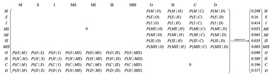
Figure 1.
DTBM of Diabetic Symptoms and Treatments.
The elements in and are 0, and the elements in and can be determined by statistics of cases. However, due to information protection measures or other reasons, it is difficult to count the medication use of a certain symptom. There is often no known statistical data on the medication use of a certain symptom in the sample, as shown in Figure 2.
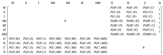
Figure 2.
Missing One Column in the DTBM.
Information on medications for dementia symptoms is missing. At this time, if we want to give the doctor data support on how to use medication for patients with dementia symptoms, we can use Formula (3) to complete the probability information of each medication regimen under dementia, as shown in Figure 3. The specific calculation is as follows:
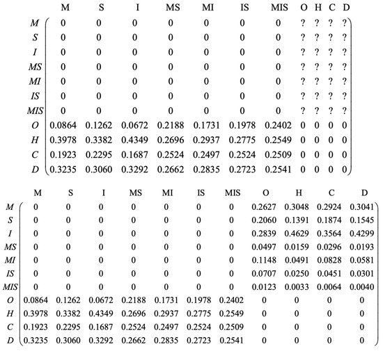
Figure 3.
Completing Missing Posterior Columns.
6.2. Posterior Columns Missing
Furthermore, if there are multiple or all missing columns in A, we need to follow Bayesian inference and supplement the entire data set according to Formula (7), as follows:
6.3. Both the Posterior and the Likelihood of Missing
Due to the low level of digitization in many areas, not only the statistics of drug therapies under various symptoms are missing, but also the statistics of the efficacy of various drugs or drug combinations on different symptoms are also missing.
What we have done is: First, establish a whole null matrix with 56 unknown elements we need; second, realize the constraint corresponds to the matrix consisting of the variable coefficient of the second and third blocks matrix A; third, build the maximize function we presented in Section 5 to approximate the 56 elements.
Finally, all unknown elements are obtained, and the distribution diagrams are shown in Figure 4, Figure 5 and Figure 6.
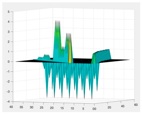
Figure 4.
Bounds of solutions.
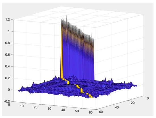
Figure 5.
Numbers of Hessian Matrices.
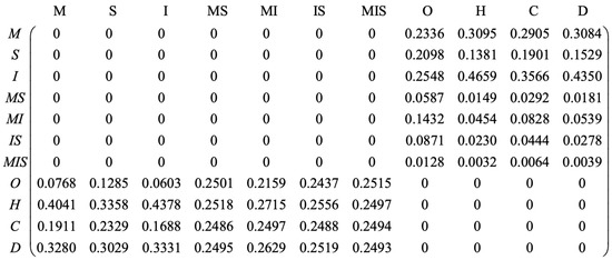
Figure 6.
Completed DTBM.
The feasible region of the solution space, as shown in Figure 4, is defined by the linear equality constraints. These constraints are represented in the form of a matrix, and they set the boundaries for the possible values that the solution can take. The constraints ensure that the solution satisfies all the necessary requirements and conditions for it to be considered a valid solution.
Figure 5 shows the matrix derivatives for searching solutions of the optimization model. By analyzing the numbers in the Hessian matrix, we can determine whether a given point is a local minimum, maximum, or saddle point. This information is crucial in finding the optimized solution, as it helps to identify the optimal point in the solution space.
Finally, all the missing probabilities we completed, shown in Figure 4, are the solutions of the maximization optimization model we mentioned before.
Programming steps:
Each of the following functions, except for the main function code2, is the function written according to various parameters required in MATLAB’s fmincon package:
Step 1. For the function boundary, the return values are beq (the value on the right side of the linear constraint equation), ub (the upper bound of the variable), lb (the lower bound of the variable), X0 (the initial value of the variable, which defaults to 0). It can be observed that the variables in each column of matrix A add up to one, and there are columns in total, so there are 1 s on the right side of the equation. In addition, according to the multiple constraints between variables (the relationship between variables in the lower left part and the upper right part of the matrix A), there are constraints in total, so there are 0 s on the right side of all equations. Thus, use a1 and a2, respectively, to realize 1 s ( rows and 1 column), 0 s ( rows and 1 column), and vertically superimpose the two columns to form the return value beq ( rows and 1 column). For each variable, the lb is 0, and the ub is 1, and there are variables in total, so the lb values are all 0 ( rows and 1 column), and the ub values are all 1 ( rows 1 column).
Step 2. For the function mat1, the purpose is to realize the constraints that the sum of the variables in each column of the matrix A is 1. Firstly, generate a zero matrix with rows and columns. It can be observed that in the first m columns of matrix A, each column has n variables that add up to 1, and in the last n columns, each column has m variables that add up to 1. Thus, using the for loop and if statement, assume that i represents the row and a acts as a positioning function with the initial value 1, which represents the first column. From row 1 to row , start with row 1; if i, then assign n elements the value of 1 and move a forward n positions; if i , then assign m elements the value of 1 and move a forward m positions.
Step 3. For the function mat2, the purpose is to realize the constraints that , where corresponds to the lower left part of the matrix A, and corresponds to the upper right part of matrix A. The return value of Mat2 corresponds to the matrix with rows and columns, which is formed by the variable coefficient in the lower left part of the matrix, A. i is the number of rows, and j is the number of columns; when i j, assign , respectively.
Step 4. For the function mat3, the purpose is to realize the constraints that , where corresponds to the lower left part of the matrix A, and corresponds to the upper right part of matrix A. The return value of Mat2 corresponds to the matrix with rows and columns, which is formed by the variable coefficient in the lower left part of the matrix, A. i is the number of rows, and j is the number of columns; when j , assign respectively.
Step 5. For the function myfun, the purpose is to construct the objective function, and the purpose of the nested function obj is to generate the target matrix A. Firstly, generate a zero matrix with rows and columns, and k acts as a positioning function with the initial value 1, which represents the first variable, j is the number of columns, and i is the number of rows. When j i , the positions on the corresponding matrix are variables from x1 to . When j and i , the positions on the corresponding matrix are variables ) to . Objective function or . Among them, each column of B is x, and there are m+ columns in total.
Step 6. For the main function code2, the values of x, m, and n need to be changed each time; x is the eigenvector, m is the first m elements of x, and n is the last n elements of x. A is a nonlinear constraint matrix, which is not involved this time. Thus, A and b are empty, mat1, mat2, and mat3 jointly generate linear constraint matrices Aeq, beq, xo, ub, and lb, and call the corresponding functions, where fun = @(X)myfun(X, x, m, n). The purpose of this processing is: the original function fun is limited to only passing in the variable parameter X, and other parameters can be passed in under the current method. Finally, bring all the parameters into fmincon to get the result; x is the variable value, and fval is the optimal value which is defaulted as the minimum value.
The results we obtained complete a whole matrix only with one eigenvector according to high-rank assumption. The completed elements are the probabilities of symptoms and medications that can support doctors in planning their treatments for diabetic patients.
7. Discussion
The results complete a probabilities matrix by one eigenvector. Fifty-six probabilities are obtained by the optimizing program. The 28 results in block 2 of the DTBM represent the conditional probabilities of each medical regimen under each symptom, while the other 28 results in block 3 of DTBM represent conditional probabilities of each symptom under each medical regimen. All the completed elements follow Bayes’ rule [14] that the eigenvector of the completed matrix is exactly what we assumed. The completed conditional probabilities can reveal the relationship between diabetes symptoms and medication regimens.
Due to the crude nature of the previous data, it is difficult to find the symptoms of each patient in the early stages of diabetes and the treatment plan given by the doctor for each characteristic. However, statistics are more readily available on the overall proportion of treatment options allocated to the case and the probability distribution of the occurrence of each symptom. The accuracy of the treatment recommendation can be significantly improved if the treatment plan for each case for each symptom is completed with known outcome information from successful treatment cases. Current research in the literature on missing value completion focuses on low-rank matrix completion methods such as alternating least squares. Alternating Least Square is doing a pretty good job at solving the scalability and sparseness of the rating data, and it’s simple and scales well to very large datasets. But Alternating Least Square or other matrix completion methods are based on matrix factorization algorithms like SVD that need to have parts of the matrix. That can not be useful in the problem of this paper that the information of matrix was all lost. Comparing the existing methods, such as alternative least squares [15], this model produced more information from less.
The produced information we found respected Shannon’s theorem [16], but at the same time, the relations between symptoms and regimens are dug out of overall links due to the eigenvectors! These relations can be used to support doctors, especially the completed conditional probabilities of regimens under each symptom. Doctors can make a medical plan according to these probabilities.
The restricted condition of our model is the probability of different symptoms in diabetic patients, and the probability of each medication regimen being used are the stable probability distributions of the symptoms and medication regimens in people with diabetes, and it mathematically conforms to the stable state theory of the Markov matrix. Based on the above information, the sum of the completed values in each column must be one, which limits this model to apply specific problems.
8. Conclusions
This article establishes a method to complete a probabilities matrix in that all the elements are missed, and it is a full rank matrix only by using one eigenvector. We assumed probabilities of symptoms and regimens given by statistic as a principle eigenvector of the DTBM, which separates symptoms and regimens as causes and effects set in block 2 and block 3 of the matrix. The Following properties of the Markov matrix, the model we proposed completed the whole matrix when it is totally missed by optimizing the eigenvalue and constraining the range of each probability [14]. The results obtained by this model satisfied Bayes’ rule and let the eigenvalue be 1 [15]. That met our assumed condition, and we finished the completed work. This work is different from the other matrix completion assuming the matrix has a low rank and musted be given parts of the completed elements in this matrix [16]. The limitation of the model is that the missing data must be probabilities of causes and effects, and it cannot be used in other kinds of problems. We assumed the data obtained from medical institutions after decades of sample statistics are the stable probability distributions of the symptoms and medication regimens.
Author Contributions
Methodology, M.L.; Resources, L.Z. and Q.Y.; Writing—original draft, M.L. and L.Z.; Writing—review & editing, Q.Y.; Supervision, L.Z.; Funding acquisition, Q.Y. All authors have read and agreed to the published version of the manuscript.
Funding
This research received no external funding.
Institutional Review Board Statement
This study did not require ethical approval.
Informed Consent Statement
Informed consent was obtained from all subjects involved in the study.
Data Availability Statement
The data that support the findings of this study are available from https://pubmed.ncbi.nlm.nih.gov/26425567/ (accessed on 27 November 2022).
Acknowledgments
We would like to thank Lingrui Xu for their valuable feedback and support throughout the writing process. Their input and insights were instrumental in shaping the direction and focus of this paper.
Conflicts of Interest
The authors declare no conflict of interest.
References
- Sillars, B.; Davis, W.A.; Hirsch, I.B.; Davis, T.M. Sulphonylurea–metformin combination therapy, cardiovascular disease and all cause mortality: The Fremantle Diabetes Study. Diabetes Obes. Metab. 2010, 12, 757–765. [Google Scholar] [CrossRef]
- Gebrie, D.; Manyazewal, T.; AEjigu, D.; Makonnen, E. Metformin-Insulin versus Metformin-Sulfonylurea Combination Therapies in Type 2 Diabetes: A Comparative Study of Glycemic Control and Risk of Cardiovascular Diseases in Addis Ababa, Ethiopia. Diabetes Metab. Syndr. Obes. Targets Ther. 2021, 14, 3345. [Google Scholar] [CrossRef]
- Naqvi, A.A.; Mahmoud, M.A.; AlShayban, D.M.; Alharbi, F.A.; Alolayan, S.O.; Althagfan, S.; Iqbal, M.S.; Farooqui, M.; Ishaqui, A.A.; Elrggal, M.E.; et al. Translation and validation of the Arabic version of the General Medication Adherence Scale (GMAS) in Saudi patients with chronic illnesses. Saudi Pharm. J. 2020, 28, 1055–1061. [Google Scholar] [CrossRef] [PubMed]
- Albahli, S. Type 2 machine learning: An effective hybrid prediction model for early type 2 diabetes detection. J. Med. Imaging Health Inform. 2020, 10, 1069–1075. [Google Scholar] [CrossRef]
- Kopitar, L.; Kocbek, P.; Cilar, L.; Sheikh, A.; Stiglic, G. Early detection of type 2 diabetes mellitus using machine learning-based prediction models. Sci. Rep. 2020, 10, 11981. [Google Scholar] [CrossRef] [PubMed]
- Pham, T.M.; Carpenter, J.R.; Morris, T.P.; Sharma, M.; Petersen, I. Ethnic differences in the prevalence of type 2 diabetes diagnoses in the UK: Cross-sectional analysis of the health improvement network primary care database. Clin. Epidemiol. 2019, 11, 1081. [Google Scholar] [CrossRef] [PubMed]
- Hastie, T.; Mazumder, R.; Lee, J.D.; Zadeh, R. Matrix completion and low-rank SVD via fast alternating least squares. J. Mach. Learn. Res. 2015, 16, 3367–3402. [Google Scholar] [PubMed]
- Vivar, G.; Kazi, A.; Burwinkel, H.; Zwergal, A.; Navab, N.; Ahmadi, S.A. Simultaneous imputation and disease classification in incomplete medical datasets using Multigraph Geometric Matrix Completion (MGMC). arXiv 2020, arXiv:2005.06935. [Google Scholar]
- Chen, J.; Xu, H.; Liu, M.; Zhang, L. Bayesian Matrix Completion for Planning Diabetes Treatment Based on Urban Cases. In Proceedings of the 2022 International Conference on Computational Infrastructure and Urban Planning, Wuhan, China, 22–24 April 2022. [Google Scholar]
- Bhattacharya, S.; Chatterjee, S. Matrix completion with data-dependent missingness probabilities. IEEE Trans. Inf. Theory 2022, 68, 6762–6773. [Google Scholar] [CrossRef]
- Bo, M.; Gallo, S.; Zanocchi, M.; Maina, P.; Balcet, L.; Bonetto, M.; Marchese, L.; Mastrapasqua, A.; Aimonino Ricauda, N. Prevalence, Clinical Correlates, and Use of Glucose-Lowering Drugs among Older Patients with Type 2 Diabetes Living in Long-Term Care Facilities. J. Diabetes Res. 2015, 2015, 174316. [Google Scholar] [CrossRef] [PubMed]
- Lei, Z.; Liu, M.; Xu, X.; Yue, Q. A Data-experience intelligent model to integrate human judging behavior and statistics for predicting diabetes complications. Alex. Eng. J. 2022, 61, 8241–8248. [Google Scholar] [CrossRef]
- Wang, L.; Peng, W.; Zhao, Z.; Zhang, M.; Shi, Z.; Song, Z.; Zhang, X.; Li, C.; Huang, Z.; Sun, X.; et al. Prevalence and treatment of diabetes in China, 2013–2018. JAMA 2021, 326, 2498–2506. [Google Scholar] [CrossRef] [PubMed]
- Young, F.W.; De Leeuw, J.; Takane, Y. Regression with qualitative and quantitative variables: An alternating least squares method with optimal scaling features. Psychometrika 1976, 41, 505–529. [Google Scholar] [CrossRef]
- Bayes, T. LII. An essay towards solving a problem in the doctrine of chances. By the late Rev. Mr. Bayes, FRS communicated by Mr. Price, in a letter to John Canton, AMFR S. Philos. Trans. R. Soc. Lond. 1763, 53, 370–418. [Google Scholar]
- Shannon, C.E. A mathematical theory of communication. Bell Syst. Tech. J. 1948, 27, 379–423. [Google Scholar] [CrossRef]


Disclaimer/Publisher’s Note: The statements, opinions and data contained in all publications are solely those of the individual author(s) and contributor(s) and not of MDPI and/or the editor(s). MDPI and/or the editor(s) disclaim responsibility for any injury to people or property resulting from any ideas, methods, instructions or products referred to in the content. |
© 2023 by the authors. Licensee MDPI, Basel, Switzerland. This article is an open access article distributed under the terms and conditions of the Creative Commons Attribution (CC BY) license (https://creativecommons.org/licenses/by/4.0/).