A Novel Fault Diagnosis of a Rolling Bearing Method Based on Variational Mode Decomposition and an Artificial Neural Network

Abstract

In recent years, artificial neural networks have been widely used in the fault diagnosis of rolling bearings. To realize real-time diagnosis with high accuracy of the fault of a rolling bearing, in this paper, a bearing fault diagnosis model was designed based on the combination of VMD and ANN, which ensures a higher fault prediction accuracy with less computational time. This paper works from two aspects, including fault feature extraction and neural network structural parameter optimization to obtain an ANN bearing fault diagnosis model with high performance. The raw vibration signals of 10 fault types were divided into training, verification and testing datasets by the random step increment slip method. The variational mode decomposition method was used to decompose the raw vibration signal into several intrinsic mode functions. A new definition of the energy of each intrinsic mode function based on discrete Fourier transform and information entropy method were used as the input for the artificial neural network. Furthermore, the structural parameters of the artificial neural network were designed to obtain a high-performance neural network. The artificial neural network used in this paper had three hidden layers and 13 neurons in each hidden layer. Compared with several machine and deep learning algorithms, the artificial neural network can better fulfill the classification task of rolling bearing fault types with a mean prediction accuracy of 99.3% and computation time of 2.4 s based on a small training dataset.

1. Introduction

Rolling bearings are important components of rotating machinery in the automotive, aviation and marine fields. The fault diagnosis of bearings is very helpful for rotating machinery to maintain safe operation with high performance. On the one hand, in practical engineering applications, the bearing vibration characteristics are vulnerable to many factors, such as internal and external noise, which results in significant challenges for the fault diagnosis of bearings’ inner and outer rings [1]. On the other hand, real-time monitoring is required to perform real-time control for engine rolling bearing components in the fault diagnosis of rolling bearings. Therefore, both the prediction accuracy and computation time should be taken into consideration in the actual application.

From the perspective of the input signal format, bearing fault diagnosis methods can be divided into raw-vibration-based methods and feature-extraction-based methods. The raw vibration signal can be directly used as input for a deep learning (DL) method because of its powerful intelligent learning and data mining ability, such as convolutional neural network (CNN) [2,3], generative adversarial network [4] and capsule neural network [5]. Of course, there are also studies that combine DL methods with feature extraction methods, such as FFP-DL [6], deep feature transfer learning [7] and reinforcement ensemble deep transfer learning network [8]. Although fault diagnosis based on DL usually has a higher prediction accuracy, it needs a great quantity of data, which results in long computational time. Therefore, many researchers try to use machine learning (ML) methods for fault diagnosis with high computational efficiency, such as RF [9], SVM [10], artificial neural network (ANN) [11] and k-nearest neighbor (KNN) [12]. In general, the fault diagnosis accuracy of ML methods is not as good as that based on a DL method. However, the advantages of ML methods are obvious, namely, simple implementation, fast computation and low demand for training data. In addition, if we can design appropriate feature extraction methods based on actual needs, the performance of ML methods would be comparable to that of DL methods.

As a classical ML framework, an ANN is still an effective mean to solve complex problems. With outstanding performance, ANNs have resulted in great successes and set new records in handling different tasks, such as the identification of handwritten numeral and target classification. It is until today that ANNs are still superior to other methods in terms of classification tasks. Compared with the DL method, the structure of an ANN is much simpler, which indicates high computational efficiency. Although the prediction accuracy of an ANN is usually not as good as that of DL methods, it can be improved significantly if the network structure is designed reasonably. Therefore, how to reasonably design a network structure to achieve high performance is the key point in solving complex problems with ANNs. However, theoretical guidance on the selection of a network structure is not available at present, and trial-and-error methods are still used to adjust the structure of ANNs in practical applications. In addition, the feature extraction of the input data is another key issue to improve an ANN’s performance. In recent years, many studies have successfully adopted an ANN for bearing fault diagnosis. Samanta applied a multilayer perceptron ANN combined with the genetic algorithm for bearing fault detection, where the genetic algorithm is used to selected the characteristic parameters of the classifiers and the input features [13]. Based on the pattern recognition technique, Kerboua proposed a novel ANN method for the fault diagnosis in induction motors [14]. Sepulveda applied an ANN to develop a vibration-based machine learning model for fault diagnosis in rotating machines, and the ANN parameters, such as the number of layers, number of neurons and types of functions, were optimized [15]. Based on the coherent composite spectrum and principal component analysis, Cao presented an automated data fusion-based gear fault classification framework with ANN for rotating machines [16]. With structural health monitoring techniques and model-based numerical approaches, Monteiro established an ANN model to predict the machine state of a gear [17]. Toma presented a classification framework with ANN for an induction motor bearing fault, and wavelet scattering transform-based features were used as the input data [18]. Tayyab applied an ANN and K-nearest neighbors to tackle the fault detection and identify the severity level of spiral bevel gears under different operating conditions [19]. Based on the feature extraction of the direct torque control and Hilbert transform, Idrissi proposed a novel ANN model for induction motor bearing fault diagnosis [20].

In this paper, an ANN was selected as the training model, which was combined with the feature extraction method of the variational mode decomposition (VMD) to perform the fault diagnosis of rolling bearings. VMD, proposed by Dragomiretskiy in 2014, is an adaptive and completely nonrecursive mode variation signal processing method [21]. VMD overcomes the problems of mode component aliasing in EMD method [22] and decomposes the signal into several signals of different frequency scales. VMD can determine the number of mode decompositions of the signal based on the actual situation and then adaptively match the best central frequency and finite bandwidth of each mode in the search and solution process, finally realizing the effective separation and frequency domain division of the intrinsic mode components in the signal. In recent years, feature extraction based on VMD has been applied more frequently in the field of fault diagnosis. Wang proposed a novel VMD based on power information for the fault diagnosis of rolling bearings [23]. Yi presented a novel VMD based on power spectral density for fault diagnosis for rolling bearing [24]. Zhang applied VMD and CNN for the fault diagnosis of a power grid [25]. Geng established a new VMD method for fault diagnosis using the combination of sparse principal component and VMD [26]. For the variable speed of rolling bearings, Sharma used VMD to obtain the weak fault features [27].

This paper realized the fault diagnosis of rolling bearings with high accuracy by designing the data preprocessing method, feature extraction and ANN structure appropriately. In terms of the preprocessing and feature extraction of a bearing’s vibration data, this paper obtained the optimal data sampling quantity and sampling period by studying the influences on them for prediction accuracy and computational time. The VMD method and discrete Fourier transform were applied to process the preprocessed data to obtain the power spectral density of the intrinsic mode functions of the bearing vibration data. Meanwhile, the normalized energy of bearing vibration data was obtained based on Shannon entropy theory. In terms of the ANN’s design, this paper took the normalized energy as the input for the ANN to train the model. This paper studied the influence of the training function, activation function, hidden layer number and node number in each hidden layer on the prediction accuracy and computation time of the model to determine the optimal ANN structure. The procedures and results of the study has certain guiding significance for bearing fault diagnosis based on ANN.

The rest of the paper is organized as follows: Section 2 presents the preprocessing of raw vibration signal, feature extraction based on VMD and construction of an ANN for fault diagnosis. Section 3 illustrates the performance of the fault diagnosis with ANN based on VMD. Section 4 provides the conclusion of this paper.

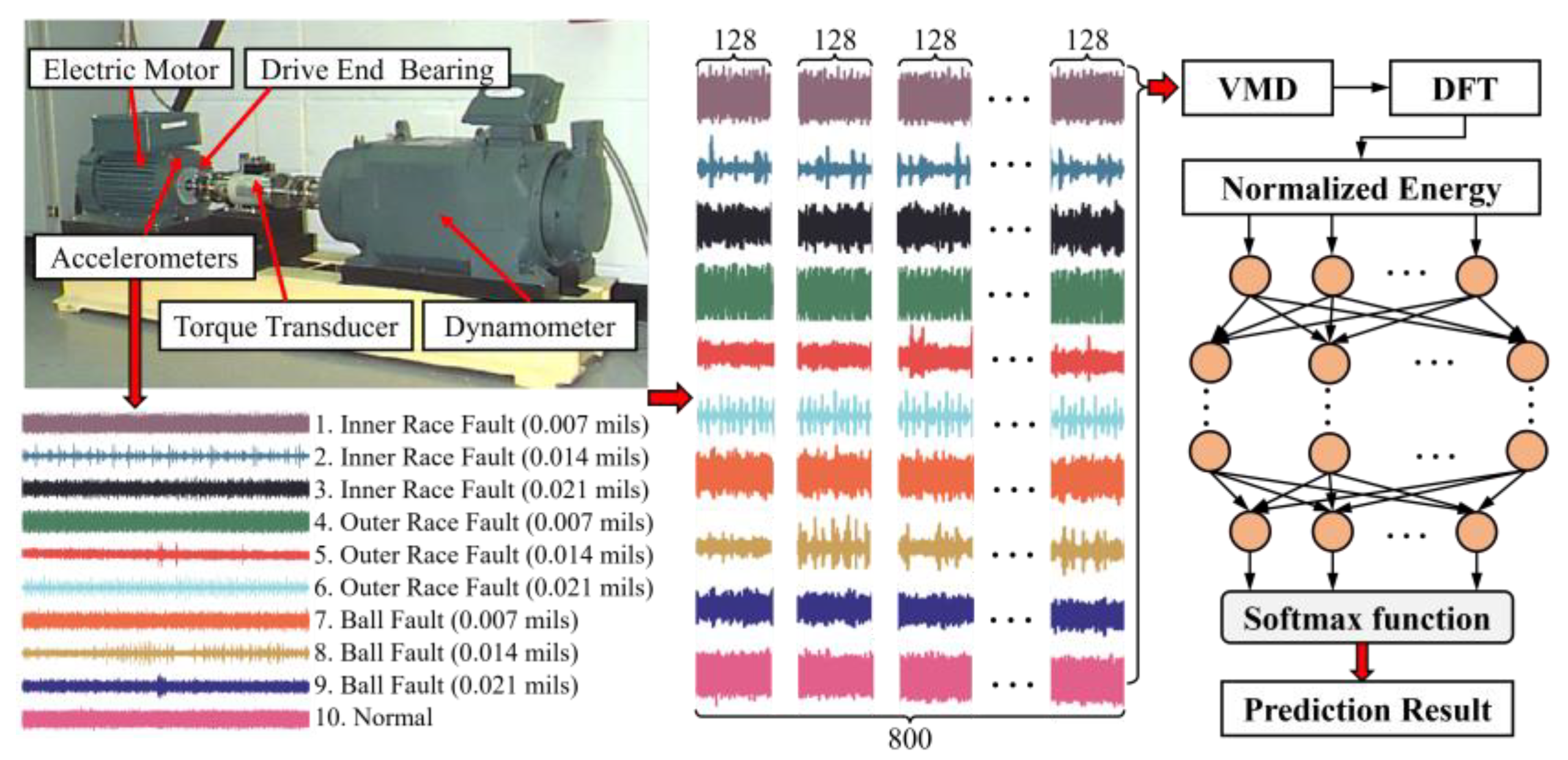
2. Fault Diagnosis of Rolling Bearing Based on VMD and ANN

2.1. Data Preprocessing

The raw vibration dataset of rolling bearings are from the Case Western Reserve University Bearing Data Center (CWRU). The dataset contains 10 rolling bearing fault states of nine fault types and one normal state. There are three kinds of fault locations in the inner race, outer race and ball. The diameters of the faults were 0.007 inches, 0.014 inches, 0.021 inches.

Table 1. Details of the dataset in the bearing fault experiment.

No.	Fault Location	d (mils)	Training Set	Validation Set	Testing Set	Target Label
1	Inner Race	0.007	500	200	100	[1 0 0 0 0 0 0 0 0 0]
2	Inner Race	0.014	500	200	100	[0 1 0 0 0 0 0 0 0 0]
3	Inner Race	0.021	500	200	100	[0 0 1 0 0 0 0 0 0 0]
4	Outer Race	0.007	500	200	100	[0 0 0 1 0 0 0 0 0 0]
5	Outer Race	0.014	500	200	100	[0 0 0 0 1 0 0 0 0 0]
6	Outer Race	0.021	500	200	100	[0 0 0 0 0 1 0 0 0 0]
7	Ball	0.007	500	200	100	[0 0 0 0 0 0 1 0 0 0]
8	Ball	0.014	500	200	100	[0 0 0 0 0 0 0 1 0 0]
9	Ball	0.021	500	200	100	[0 0 0 0 0 0 0 0 1 0]
10	Normal	Normal	500	200	100	[0 0 0 0 0 0 0 0 0 1]

Here, d denotes the fault diameter.

shows the details of the fault dataset in the bearing fault experiment. The sampling frequency of the rolling bearing vibration signal was 48 kHz.

For one type of bearing fault status, the random step increment slip method [28] was used to intercept and divide each vibration signal into 700 groups of training samples and 100 groups of testing samples, as shown in Figure 1. A new sample was obtained by a random start point, and the next random start point slips with a certain distance increment. For each raw vibration signal of the 10 fault types, 1024 points were collected as the training data. For the 10 types of fault types, we obtained a shape of 8000 × 1024 training data and a shape of 8000 × 10 labels of the fault types represented by a one-hot code. Moreover, the min–max normalization method was adopted to map the vibration signals to interval [0, 1]. Finally, the raw vibration signal was divided into 500 groups of training samples, 200 groups of validation samples and 100 groups of testing samples for each fault type.

To study the influences of the sample quantity and sampling period on the prediction accuracy and computation time of the proposed method, we processed the vibration data of rolling bearings from two aspects. On the one hand, to study the sample quantity’s influences on the model’s performance, it extracted samples with the number ranging from 5000 to 30,000 as the input for the model to explore the sample number’s influences on the prediction accuracy and computation time of the model. As shown by the research results in Section 3.3, the optimal sample number for fault diagnosis based on VMD and ANN was 8000. On the other hand, the impact of the sampling period on the fault classification accuracy and computation time was studied. As shown in Figure 1, the length of every sampling point for the data on bearing faults was 1024. The resampling of all fault data was carried out to attain the sampling data of different sampling periods, with the specific procedure shown in Figure 2. Though our investigation, it was found that when the sampling period was 1/6 ms, the classification accuracy of the bearing faults would be maximized and the computation time would be minimized. Therefore, the optimal sampling period in this paper is defined as 1/6 ms.

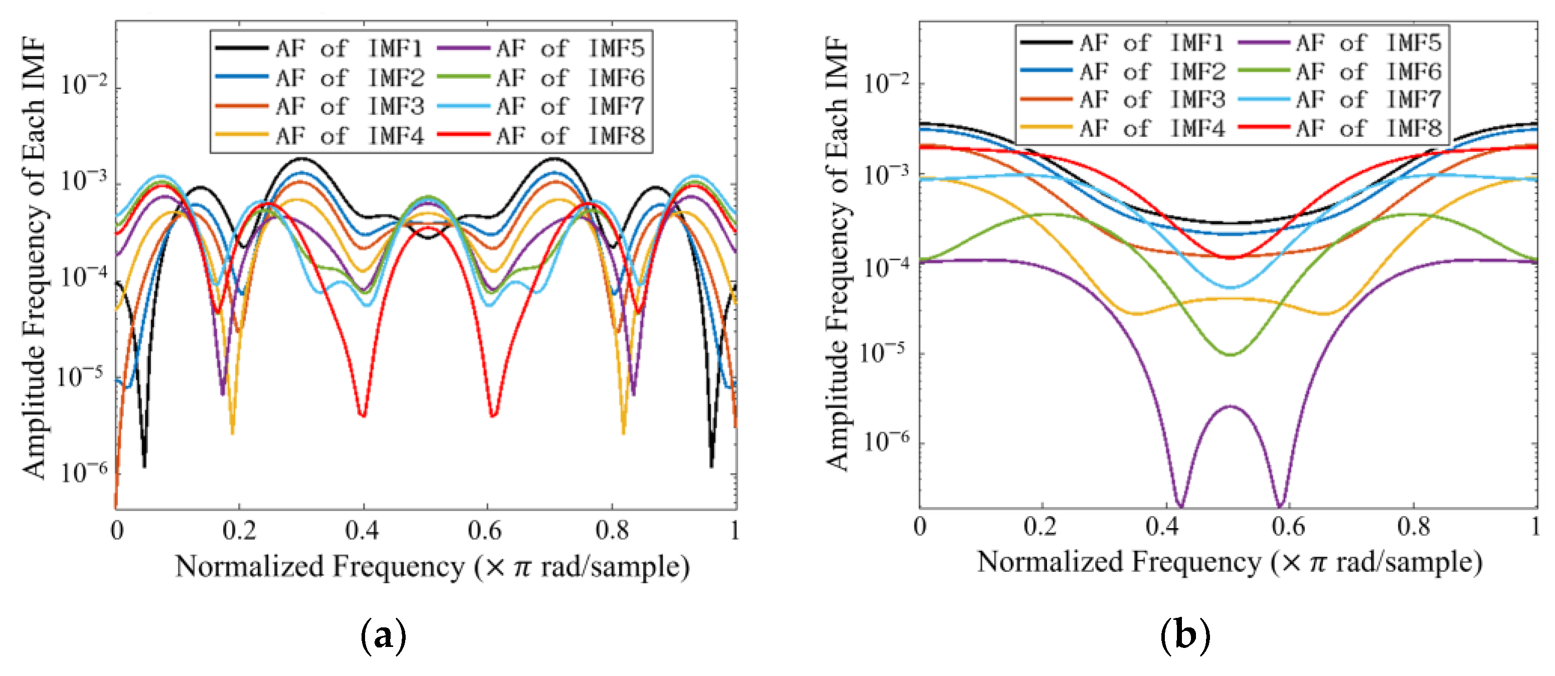
2.2. Feature Extraction Based on VMD

The variational mode decomposition (VMD) decomposes the raw vibration signal of a bearing x(t) into several numbers, N, of intrinsic mode functions (IMFs), $u_k\left(t\right)$ [21]:

$$x\left(t\right)={\displaystyle \sum }_{k=1}^K{u}_k\left(t\right)=A_k\left(t\right)\cos \left({\varphi }_k\left(t\right)\right)$$

(1)

where $k=1, 2, \dots , 8$ is the number of the decomposed IMFs, ${\varphi }_k\left(t\right)$ is mode phase and $A_k\left(t\right)$ is the envelope. To obtain the IMFs, $u_k\left(t\right)$, and central frequency, $f_k$, the optimum of the augmented Lagrangian was performed as follows:

$$\begin{gathered} L\left(u_k\left(t\right), f_k, {\lambda }_t\right)=\alpha {\displaystyle \sum }_{k=1}^K\Vert \frac{d}{dt}\left[\left(\delta \left(t\right)+\frac{j}{\pi t}\right)\times u_k\left(t\right)\right]e^{-j2\pi f_{k}t}{\Vert }_2^2 \\ +\Vert x\left(t\right)-{\displaystyle \sum }_{k=1}^K{u}_k\left(t\right){\Vert }_2^2+{\lambda }_t, x_t-{\displaystyle \sum }_{k=1}^K{u}_k\left(t\right) \end{gathered}$$

(2)

where ${\lambda }_t$ is the Lagrangian coefficient, $\alpha$ is the scale factor, $\delta$ is the Fermi–Dirac distribution, $\Vert ·{\Vert }_2^2$ is the 2-norm and $\langle ·\rangle$ is the inner product. The VMD method captures the mode waveforms and central frequencies of the raw rolling bearing vibration signal in the frequency domain.

The VMD method extends the signal by mirroring half of its length on both sides. As shown in Figure 3, the vibration signal with 1024 sampling points was decomposed to obtain eight IMF components. The waveforms and central frequencies of the eight IMFs clearly differed from each other. As shown by the study, defining an appropriate sampling period could not only guarantee the fault classification result with high accuracy but also reduce the computation time of the algorithm. As shown in Figure 2, the optimal sampling period in this paper was 1/6 ms, that is, 128 sampling points. Therefore, after resampling and VMD processing, 1024 sampling points of each raw vibration signal became 128 points.

In order to capture the quantization features, discrete Fourier transform (DFT) was performed on the eight IMFs to obtain the amplitude frequency of each IMF, as follows:

$$X_k\left(f\right)=\frac{1}{N}{\displaystyle \sum }_{n=0}^{N-1}{u}_k\left(n\right)e^{-j\pi nf/N}$$

(3)

where $X_k\left(f\right)$ is the amplitude frequency of each IMF, n is the length of each IMF and N = 128. According to Equation (3), the discrete Fourier transform results of the eight IMFs are shown in Figure 4.

Furthermore, inspired by Shannon entropy, a newly defined energy was used to characterize the central frequency and amplitude frequency features of each IMF. The new defined energy, E, of each IMF’s amplitude frequency was calculated using the equation below:

$$E_k=-{\displaystyle \sum }_{n=0}^N{f}_n\times {\log }_{10}\left(X_k\left(f_n\right)\right)$$

(4)

where k = 1, 2, ..., 8 is the index of the eight IMF components, n = 1, 2, …, 128 is the signal length of each IMF component and $X_k\left(f\right)$ is the amplitude frequency of the IMFs corresponding to frequency f. Then, the total energy was obtained using the following equation:

$$E={\displaystyle \sum }_{k=1}^8{E}_k$$

(5)

The normalized energy eigenvector of each IMF’s amplitude frequency can be obtained using:

$$X=\left[\frac{E_1}{E}, \frac{E_2}{E}, \dots ,\frac{E_8}{E} \right]$$

(6)

The normalized energy eigenvector $X$ contains the signal characteristics of the raw vibration signal at different time scales. In addition, taking the normalized energy eigenvector of each IMF amplitude frequency as the input for the ANN can not only improve the prediction accuracy of the bearing fault type but also reduce the data size and, thus, improve the computational efficiency.

2.3. Architecture of the Artificial Neural Network

Because of their strong capacity for adaptation and self-organization and nonlinear mapping ability, ANNs have been widely used in the fault diagnosis of bearings. There are many ANN structures, such as a linear ANN, backpropagation ANN, radial basis function ANN and probabilistic neural network. A linear ANN uses the least mean square training function to adjust the weight and bias of the network. Although the computational speed of a linear ANN is very fast, it is only suitable for tackling linear separable problems. A radial basis function ANN and probabilistic neural network have fast convergence speed, but their prediction accuracy is not ideal for the prediction of bearing fault diagnosis [13]. A BP ANN is a kind of multilayer perceptron, which is the most widely used neural network structure at present. Therefore, this paper applied a BP ANN to perform the fault diagnosis of rolling bearings.

A brief flowchart of the ANN is shown in Figure 5. The input for the ANN was the normalized energy of each IMF’s amplitude frequency. The shape of the total input feature data was 8000 × 8. The target input data were labels of the bearing fault types represented by a one-hot code with the shape of 8000 × 10. The neuron nodes of the input and output layers were 8 and 10, respectively, which correspond to the 8 normalized energy features of the input data and 10 fault types of rolling bearings. The number of hidden layer was three, and each hidden layer contained 13 neurons. The error was used for the fault diagnosis. The soft-max activation function was applied for the fault type classification of rolling bearings in the output layer. The output of the ANN was fed into the soft-max activation function to judge the bearing fault type according to the 10 probability values.

The implementation and training process of the proposed method was conducted with MATLAB on a computer with a i7-6700 CPU and 32 GB memory. The ANN architecture built using MATLAB is shown in Figure 6. The input data were divided into a training dataset, validation dataset and testing dataset. The parameters of the ANN, such as the number of hidden layer, number of neuron nodes and training function, were optimized using a trial-and-error method for the different fault types of rolling bearings.

The performance of an ANN is mainly affected by the number of hidden layers, number of neuron nodes in each hidden layer and the training function. In order to simplify the parameter optimization of the ANN, each hidden layer had the same number of neuron nodes. The prediction accuracy for the number of hidden layers, ranging from 1 to 5, and the number of neurons in each layer, ranging from 5 to 15, were studied in this paper. The training functions, including Levenberg–Marquardt, Bayesian regularization, BFGS quasi-Newton, resilient backpropagation and scaled conjugate gradient, were used to build the ANN. Through our studies, we found that the Bayesian regularization training function performs the best.

In addition, the commonly used activation functions included sigmoid, tanh, ReLU, leaky ReLU and ELU. Through research, it was found that these activation functions have little impact on the prediction accuracy of fault diagnosis. Therefore, the ReLU activation function with high computational efficiency was used in the input and the hidden layers of the ANN. The optimal parameters for an ANN used for rolling bearing fault diagnosis are shown in

Table 2. The optimal parameters of the ANN used for the fault diagnosis of rolling bearings.

Number of Samples	8000
Number of Neuron Nodes in the Input Layer	8
Number of Hidden Layers	3
Number of Neuron Nodes in the Hidden Layer	13
Number of Neuron Nodes in the Output Layer	10
Activation Function of the Input/Hidden Layers	ReLU
Activation Function of the Output Layer	Soft-max
Training Function	Bayesian Regularization

.

2.4. Fault Diagnosis Experiment and Analysis of Rolling Bearings

To verify the effectiveness of the proposed rolling bearing fault diagnosis method based on VMD and an ANN, this paper designed test and analysis procedures for the rolling bearing fault, as shown by Figure 7. Among others, the Case Western Reserve University (CWRU) bearing vibration signals was taken as the test data and test bed. The test procedures for the experiment mainly included data acquisition, data preprocessing, fault feature extraction and fault diagnosis.

The test bed for the rolling bearing damage was mainly composed of an electric motor, rolling bearings, accelerometers, torque transducer and dynamometer. The damage was located at the drive end bearing. The sampling frequency and spindle speed were 48 kHz and 1796 r/min, respectively. The accelerometers were mounted at the 12 o’clock position at the drive end of the motor housing. The fault vibration data were acquired through the accelerometers and stored in a MATLAB data format.

After attaining the original data on the rolling bearing faults, the data preprocessing method, as shown in Figure 1 and Figure 2, were applied to split the original data of each fault into 800 fault data, with each fault data containing 128 data points. Furthermore, the VMD and discrete Fourier transform methods were used to attain the normalized energy of the fault data. The normalized energy and fault label were taken as the input of the ANN to train the neural network. Finally, the training process was performed to obtain the prediction ANN model of the rolling bearing fault types.

3. Results and Discussion

3.1. Comparison of the Feature Extraction Methods

The performance of the VMD and empirical mode decomposition (EMD) in feature extraction is first compared. As shown in Figure 8a, one raw vibration signal was decomposed into eight IMFs by EMD. The mode waveforms and central frequencies were mostly concentrated in the first three IMFs, while the last five IMFs almost contained a few signal features. The amplitude of the IMFs based on the EMD method varied greatly, and most of the signal energy was concentrated in IMF1. The frequency variation based on the EMD method was also large, which led to the result that most of the signal energy was concentrated in IMF1 and IMF2. However, as shown in Figure 8b, the same raw vibration signal was decomposed into eight IMFs by VMD, and these eight IMFs contained effective waveforms and central frequencies features. The frequency of the IMFs based on VMD showed a steady gradient decrease, while the amplitude of each IMF was consistent on the whole, which ensured that every IMF contained the effective features of the raw vibration signal.

Discrete Fourier transform was performed on the eight IMFs decomposed by EMD and VMD. According to Equation (4), the energies of each IMF were calculated, as shown in Figure 9. Compared with EMD, the signal energy based on VMD had more intuitive differentiation. Therefore, the VMD method was superior to the EMD method in feature extraction.

The signal energy of eight IMFs corresponding to 10 types of bearing fault signals was calculated according to Equation (4) to further compare the feature extraction ability of EMD and VMD. As shown in Figure 10, the regularity of the energy feature extracted by the EMD method was not as obvious as that of the VMD method. Compared with EMD, the extracted energy feature based on the VMD method changed more regularly with the IMFs as a whole, which is conducive to finding the internal principle of the bearing fault in the training process of the ANN. In addition, for the extracted energy feature based on EMD, the energy of the first three IMFs was obviously larger than that of the last five IMFs based on EMD, which may count against the subsequent ANN training process.

Furthermore, with the features extracted through the raw vibration signal, EMD and VMD as the input for the ANN, the results of the prediction accuracy and computation time of bearing fault diagnosis were obtained to demonstrate the superiority of the VMD. The architecture of the ANN adopted the parameters shown in Table 2. As shown in Figure 11, the ANN based on the VMD method had the highest prediction accuracy of 99.3%, with a computation time of 2.4 s, and the prediction accuracy based on the EMD method was 94.2%, with a computation time of 2.3 s. In terms of the computation time, there was little difference between the VMD method and the EMD method. The ANN based on the raw vibration signal of the rolling bearings not only had the lowest prediction accuracy of 81.2% but also had the longest computation time of 5.6 s. Therefore, feature extraction based on VMD plays a key role in improving the performance of ANNs.

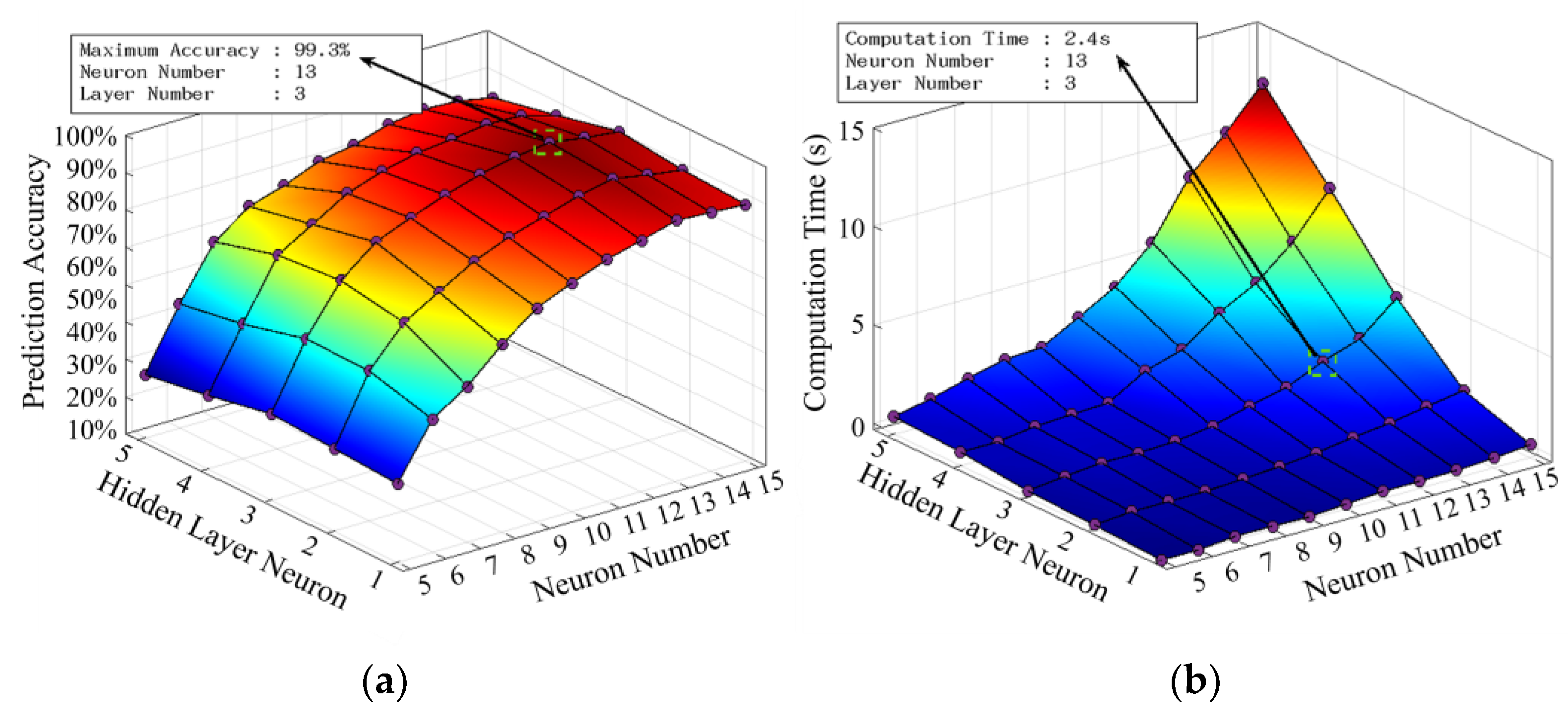
3.2. Determination of the Neural Network Architecture

The performance of the ANN was mainly affected by the format of the training data, size of the hidden layers and the training function. This section mainly explores the influence of the training functions and the size of the hidden layers on the performance of the ANN.

There are many training functions for ANNs, such as Levenberg–Marquardt (LM), Bayesian regularization (BR), BFGS quasi-Newton (BFGS-QN), resilient backpropagation (RB) and scaled conjugate gradient (SCG). These training functions have distinctive characteristics. For instances, the LM algorithm is fast with high accuracy; the BR algorithm takes longer but may process complicated problems; and the SCG algorithm uses less memory, etc. The architecture of the ANN applied the parameters shown in Table 2. Each training function was simulated 10 times, and the average values of the prediction accuracy, iteration error and computation time corresponding to each training function were obtained, as shown in Figure 12.

As shown in Figure 12, the BR training function had the highest prediction accuracy of 99.3% and the smallest training error. Although the computation time of the BR training function was 2.4 s, it is feasible in many practical engineering applications. Therefore, the BR training function was used as the training function of the ANN considering its high accuracy.

In addition, the size of the hidden layers included the number of hidden layers and the number of neurons in each hidden layers. The prediction accuracy corresponding to the number of hidden layers, ranging from 1 to 5, and the number of neurons in each layer, ranging from 5 to 15, were studied. The average value of the prediction accuracy and computation time were obtained through 10 ANN training processes. The influence of the number of hidden layers and number of neurons on the ANN’s performance is shown in Figure 13. The prediction accuracy was the highest when the number of hidden layers was three and the number of neurons in each layer was 13. Meanwhile, the computation time rose with the increase in the number of hidden layers and neurons. The computation time of the ANN with three hidden layers and 13 neurons was 2.4 s, which satisfies most of the requirements of actual engineering applications.

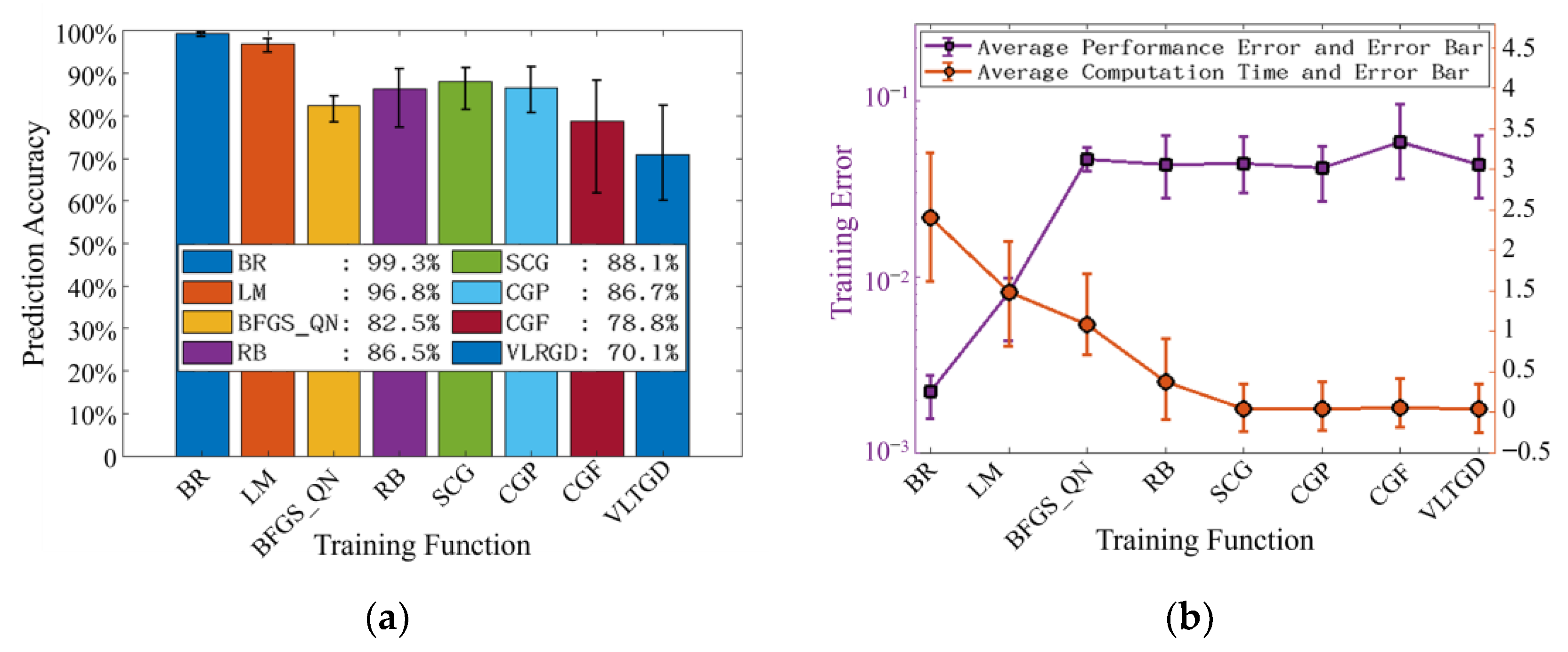
3.3. Comparison between the Proposed Method and Several Artificial Intelligence Algorithms

This part mainly compares the proposed method with several artificial intelligence algorithms in terms of their performance in the fault diagnosis of rolling bearings. Firstly, the fault prediction performance of the proposed method was compared with deep learning methods, such as 1D CNN and LTSM. The input data of the 1D CNN and LTSM were the raw vibration signal. The optimal number of samples for the 1D-CNN was 24,000, and the shape of its input data was 24,000 × 1024. The optimal number of samples for the LTSM was 22,000, and the shape of its input data was 22,000 × 1024. The architecture parameters of the 1D CNN and LSTM are shown in

Table 3. The architecture parameters of 1D CNN.

No.	Layers	Kernel Size	Kernel No.	Stride	Padding	Activation	Output
1	Conv1D	20 × 1	32	8	10	ReLU	128 × 32
2	Max Pooling	4 × 1	32	4	0	-	32 × 32
3	Flattening	-	-	-	-	-	1024
4	FC	100	1	-	-	ReLU	100 × 1
5	Output	10	1	-	-	Soft-max	10

Conv1D, 1D convolution neural networks; FC, fully connected.

and

Table 4. The architecture parameters of the LSTM.

No.	Layers	Kernel Size	Kernel No.	Activation	Output
1	LSTM	1	32	Tanh	1024 × 32
2	Flattening	-	-	-	32,768
3	FC	32	1	ReLU	32 × 1
4	Output	10	1	Soft-max	10

FC, fully connected.

, respectively.

The influence of number of samples, ranging from 5000 to 30,000, on the algorithm’s performance is shown in Figure 14. In terms of the fault diagnosis based on VMD and an ANN, its prediction accuracy reached the maximum value of 99.3% when the sample number was 8000. In addition, the prediction accuracy did not rise with the increase in the number of samples after the peak point. Therefore, the number of samples selected for this paper for the training data was 8000. In comparison, the number of samples for the CNN and LSTM in attaining maximum the prediction accuracy were 24,000 and 22,000, respectively. The increase in the number of samples for the CNN and LSTM led to an increase in the computation time.

Then, to further verify the superiority of the proposed method, it was compared with the other five artificial intelligence fault diagnosis methods for rolling bearings with the same CWRU bearing vibration signal dataset. These five fault diagnosis methods for rolling bearings include the ensemble deep neural network and CNN (CNN-EPDNN) method [29], long short-term memory with multichannel continuous wavelet transform (LSTM-MCCWT) method [30], weighted k-nearest neighbor (WKNN) method [31], medium Gaussian support vector machine (MG-SVM) method [32] and rotation forest with principal component analysis (PCA-RF) method [33]. With the i7-6700 CPU and 32 GB memory, the implementation and training process of these methods were conducted with MATLAB machine learning and deep learning toolboxes for the CWRU bearing vibration dataset with a load of 0HP and a sampling frequency of 48 kHz. As shown in Figure 15, the proposed method in this paper featured a higher prediction accuracy of 99.3% and a lower computation time of 2.4 s in comparison with the CNN-EPDNN method and LSTM-MCCWT method. Meanwhile, although the computation time of the proposed method was more than the other machine learning methods, such as WKNN, MG-SVM and PCA-RF, its prediction accuracy was obviously higher.

As shown in Figure 16, the confusion matrix of the testing dataset clearly illustrates the prediction accuracy of the different fault types, and the total prediction accuracy of the 10 fault types was 99.3%. The prediction accuracy of the proposed method for most of the fault types was 100%, and the worst prediction accuracy was 97% for condition 3 (inner race fault with a 0.021 mils fault diameter). Although the prediction accuracy of CNN can be improved by optimizing the structure; this is usually at the expense of a longer computation time. In addition, the training process of a complex DL structure needs more training data. Therefore, the proposed method can accurately identify the fault types of rolling bearings with less computation time and a smaller sized dataset.

4. Conclusions

This paper proposes a novel method based on VMD and ANN for the fault diagnosis of rolling bearings. To begin, the proposed method decomposed the raw vibration by VMD and obtained the energy of each IMF. Then, a newly defined energy feature of the IMFs was applied as the input for the ANN, which can not only reduce the computation time but also obtain accurate classification results of the fault type. Compared with EMD, the VMD method decomposed the mode waveforms and central frequencies of the raw vibration signal into each IMF more effectively such that the ANN can better classify the fault types of rolling bearings. Furthermore, the structural parameters of the ANN (training function, number of hidden layers and number of neurons in each hidden layer) were optimized to achieve an accurate fault diagnosis with less computation time. Finally, the paper studied the number of samples’ influence on the performance of the proposed method and compared the performance between the proposed method and several artificial intelligence algorithms. As shown by the research results, the proposed method can well fulfill the classification task of rolling bearing faults with higher prediction accuracy and less computation time based on a small training dataset. Therefore, it has superiority in handling actual fault prediction tasks, with high demand in real-time performance and a small training dataset.

References

1. Xie, K.; Liu, L.-C.; Li, X.-P.; Zhang, H.-L. Non-contact resistance and capacitance on-line measurement of lubrication oil film in rolling element bearing employing an electric field coupling method. Measurement 2016, 91, 606–612. [Google Scholar] [CrossRef]
2. Ruan, D.; Wang, J.; Yan, J.; Gühmann, C. CNN parameter design based on fault signal analysis and its application in bearing fault diagnosis. Adv. Eng. Inform. 2023, 55, 101877. [Google Scholar] [CrossRef]
3. Wang, X.; Mao, D.X.; Li, X.D. Bearing fault diagnosis based on vibro-acoustic data fusion and 1D-CNN network. Measurement 2021, 173, 108518. [Google Scholar] [CrossRef]
4. Zhao, B.X.; Qi, Y. Improved generative adversarial network for vibration-based fault diagnosis with imbalanced data. Measurement 2021, 169, 108522. [Google Scholar] [CrossRef]
5. Chen, T.Y.; Wang, Z.H.; Yang, X.; Jiang, K. A deep capsule neural network with stochastic delta rule for bearing fault diagnosis on raw vibration signals. Measurement 2019, 148, 106857. [Google Scholar] [CrossRef]
6. Xie, T.; Xu, Q.; Jiang, C.; Lu, S.; Wang, X. The fault frequency priors fusion deep learning framework with application to fault diagnosis of offshore wind turbines. Renew. Energy 2023, 202, 606–612. [Google Scholar] [CrossRef]
7. Yu, X.; Liang, Z.; Wang, Y.; Yin, H.; Liu, X.; Yu, W.; Huang, Y. A wavelet packet transform-based deep feature transfer learning method for bearing fault diagnosis under different working conditions. Measurement 2022, 201, 111597. [Google Scholar] [CrossRef]
8. Li, X.; Jiang, H.; Xie, M.; Wang, T.; Wang, R.; Wu, Z. A reinforcement ensemble deep transfer learning network for rolling bearing fault diagnosis with Multi-source domains. Adv. Eng. Inform. 2022, 51, 101480. [Google Scholar] [CrossRef]
9. Dong, X.; Li, G.L.; Jia, Y.H.; Xu, K. Multiscale feature extraction from the perspective of graph for hob fault diagnosis using spectral graph wavelet transform combined with improved random forest. Measurement 2021, 176, 109178. [Google Scholar] [CrossRef]
10. Wei, J.; Huang, H.; Yao, L.; Hu, Y.; Fan, Q.; Huang, D. New imbalanced bearing fault diagnosis method based on Sample-characteristic Oversampling TechniquE (SCOTE) and multi-class LS-SVM. Appl. Soft. Comput. 2021, 101, 107043. [Google Scholar] [CrossRef]
11. Kumar, R.S.; Raj, I.G.C.; Alhamrouni, I.; Saravanan, S.; Prabaharan, N.; Ishwarya, S.; Gokdag, M.; Salem, M. A combined HT and ANN based early broken bar fault diagnosis approach for IFOC fed induction motor drive. Alex. Eng. J. 2023, 66, 15–30. [Google Scholar] [CrossRef]
12. Su, Z.A.; Tang, B.P.; Ma, J.H.; Deng, L. Fault diagnosis method based on incremental enhanced supervised locally linear embedding and adaptive nearest neighbor classifier. Measurement 2014, 48, 136–148. [Google Scholar] [CrossRef]
13. Samanta, B.; Al-Balushi, K.R.; Al-Araimi, S.A. Artificial neural networks and genetic algorithm for bearing fault detection. Soft Comput. 2006, 10, 264–271. [Google Scholar] [CrossRef]
14. Kerboua, A.; Kelailia, R.; Metatla, A.; Batouche, M. Fault diagnosis in induction motor using pattern recognition and neural networks. In Proceedings of the 2018 International Conference on Signal, Image, Vision and their Applications (SIVA), Guelma, Algeria, 26–27 November 2018; pp. 1–7. [Google Scholar] [CrossRef]
15. Sepulveda, N.E.; Sinha, J. Parameter optimisation in the vibration-based machine learning model for accurate and reliable faults diagnosis in rotating machines. Machines 2020, 8, 66. [Google Scholar] [CrossRef]
16. Cao, R.F.; Kaltungo, A.Y. An automated data fusion-based gear faults classification framework in rotating machines. Sensors 2021, 21, 2957. [Google Scholar] [CrossRef]
17. Monteiro, R.d.P.; Marra, A.L.; Vidoni, R.; Garcia, C.; Concli, F. A hybrid finite element method–analytical model for classifying the effects of cracks on gear train systems using artificial neural networks. Appl. Sci. 2022, 12, 7814. [Google Scholar] [CrossRef]
18. Toma, R.N.; Gao, Y.; Piltan, F.; Im, K.; Shon, D.; Yoon, T.H.; Yoo, D.-S.; Kim, J.-M. Classification framework of the bearing faults of an induction motor using wavelet scattering transform-based features. Sensors 2022, 22, 8958. [Google Scholar] [CrossRef]
19. Tayyab, S.M.; Chatterton, S.; Pennacchi, P. Fault Detection and severity level edentification of spiral bevel gears under different operating conditions using artificial intelligence techniques. Machines 2021, 9, 173. [Google Scholar] [CrossRef]
20. El Idrissi, A.; Derouich, A.; Mahfoud, S.; El Ouanjli, N.; Chantoufi, A.; Al-Sumaiti, A.S.; Mossa, M.A. Bearing fault diagnosis for an induction motor controlled by an artificial neural network—Direct torque control using the Hilbert transform. Mathmatics 2021, 10, 42588. [Google Scholar] [CrossRef]
21. Dragomiretskiy, K.; Zosso, D. Variational mode decomposition. IEEE Trans. Signal Process. 2014, 22, 531–534. [Google Scholar] [CrossRef]
22. Huang, N.E.; Shen, Z.; Long, S.R.; Wu, M.C.; Shih, H.H.; Zheng, Q.; Yen, N.-C.; Tung, C.C.; Liu, H.H. The empirical mode decomposition and the Hilbert spectrum for nonlinear and non-stationary time series analysis. Proc. R. Soc. Lond. Ser. A Math. Phys. Eng. Sci. 1998, 454, 154–196. [Google Scholar] [CrossRef]
23. Wang, X.L.; Shi, J.C.; Zhang, J. A power information guided-variational mode decomposition (PIVMD) and its application to fault diagnosis of rolling bearing. Digit. Signal Process. 2022, 132, 103814. [Google Scholar] [CrossRef]
24. Yi, C.; Wang, H.; Ran, L.; Zhou, L.; Lin, J.H. Power spectral density-guided variational mode decomposition for the compound fault diagnosis of rolling bearings. Measurement 2022, 199, 111494. [Google Scholar] [CrossRef]
25. Zhang, Q.; Ma, W.H.; Li, G.L.; Ding, J.J.; Xie, M. Fault diagnosis of power grid based on variational mode decomposition and convolutional neural network. Electr. Pow. Syst. Res. 2022, 208, 107871. [Google Scholar] [CrossRef]
26. Geng, Z.Q.; Duan, X.Y.; Han, Y.M.; Liu, F.F. Novel variation mode decomposition integrated adaptive sparse principal component analysis and it application in fault diagnosis. ISA Trans. 2022, 128, 21–31. [Google Scholar] [CrossRef]
27. Sharma, V.; Parey, A. Extraction of weak fault transients using variational mode decomposition for fault diagnosis of gearbox under varying speed. Eng. Fail. Anal. 2020, 107, 104204. [Google Scholar] [CrossRef]
28. Zhang, Y.-D.; Yang, Z.-J.; Lu, H.-M.; Zhou, X.-X.; Phillips, P.; Liu, Q.-M.; Wang, S.-H. Facial emotion recognition based on biorthogonal wavelet entropy, fuzzy support vector machine, and stratified cross validation. IEEE Access 2016, 4, 8375–8385. [Google Scholar] [CrossRef]
29. Li, H.M.; Huang, J.Y.; Ji, S.W. Bearing fault diagnosis with a feature fusion method based on an ensemble convolutional neural network and deep neural network. Sensors 2019, 19, 2034. [Google Scholar] [CrossRef] [Green Version]
30. Gao, D.W.; Zhu, Y.S.; Ren, Z.J.; Yan, K.; Kang, W. A novel weak fault diagnosis method for rolling bearings based on LSTM considering quasi-periodicity. Knowledge-Based Syst. 2021, 231, 107413. [Google Scholar] [CrossRef]
31. Wang, Q.F.; Wang, S.; Wei, B.K.; Chen, W.W. Weighted K-NN classification method of bearings fault diagnosis with multi-dimensional sensitive features. IEEE Accesss 2021, 9, 45428–45440. [Google Scholar] [CrossRef]
32. Lin, S.L. Application of machine learning to a medium gaussian support vector machine in the diagnosis of motor bearing faults. Electronics 2021, 10, 2266. [Google Scholar] [CrossRef]
33. Kavathekar, S.; Upadhyay, N.; Kankar, P.K. Fault classification of ball bearing by rotation forest technique. Procedia Technol. 2016, 23, 187–192. [Google Scholar] [CrossRef] [Green Version]
Figure 1. The data partition method for the bearing vibration data of the different fault types.
Applsci 13 03413 g001
Figure 2. The resampling method for obtaining different sampling periods.
Applsci 13 03413 g002
Figure 3. The 8 IMFs of the vibration signal with the 1024 samples based on VMD.
Applsci 13 03413 g003
Figure 4. The amplitude frequency of each IMF based on discrete Fourier transform. AF, amplitude frequency.
Applsci 13 03413 g004
Figure 5. The brief flowchart of the ANN used in this paper.
Applsci 13 03413 g005
Figure 6. The ANN built using MATLAB for the architecture parameter optimization.
Applsci 13 03413 g006
Figure 7. Flow process diagram of the fault diagnosis experiment and analysis.
Applsci 13 03413 g007
Figure 8. Comparison of the decomposition performance of EMD and VMD on the time domain: (a) 8 IMFs decomposed by EMD in the time domain; (b) 8 IMFs decomposed by VMD in time domain.
Applsci 13 03413 g008
Figure 9. The discrete Fourier transform of the IMFs decomposed by EMD and VMD: (a) discrete Fourier transform of the IMFs decomposed by EMD; (b) discrete Fourier transform of the IMFs decomposed by VMD.
Applsci 13 03413 g009
Figure 10. Normalized energy of the IMFs corresponding to the fault types based on EMD and VMD: (a) normalized energy of the IMFs corresponding to the fault types based on EMD; (b) normalized energy of the IMFs corresponding to the fault types based on VMD.
Applsci 13 03413 g010
Figure 11. The prediction accuracy and computation time based on features extracted by VMD, EMD and raw vibration signal.
Applsci 13 03413 g011
Figure 12. Effect of the training function on the ANN’s performance: (a) prediction accuracy of the different training functions; (b) training error and computation time of the different training functions.
Applsci 13 03413 g012
Figure 13. The influence of the number of hidden layers and number of neurons on the ANN’s performance: (a) influence of the number of hidden layers and number of neurons on the prediction accuracy; (b) influence of the number of hidden layers and number of neurons on the computation time.
Applsci 13 03413 g013
Figure 14. The influence of the number of samples on the algorithm’s performance: (a) influence of the number of samples on the prediction accuracy; (b) influence of the number of samples on the computation time.
Applsci 13 03413 g014
Figure 15. The performance of the proposed method compared with other artificial intelligence methods.
Applsci 13 03413 g015
Figure 16. The confusion matrix of the fault diagnosis accuracy results for the proposed method.
Applsci 13 03413 g016