1. Introduction
Tennis is gaining popularity as a fashionable aerobic sport, and the number of tennis enthusiasts is increasing yearly. Despite the popularity of tennis, the experience of the sport is hampered by the large number of tennis balls picked up from the court, which significantly affects the enthusiasts’ enthusiasm. Most of the traditional tennis ball picking devices are mainly human-driven and require manual intervention, relying on the downward pressure action of the arm to pick up the tennis balls, which requires multiple repetitions of the arm lifting action during the picking process, wasting a lot of time and energy and being less efficient. To solve the problem of the low efficiency of manual ball pickup, the mainstream tennis ball pickup devices on the market are mainly divided into multi-degree-of-freedom-based robotic arm pickup, impeller rotation-based inhalation pickup, and motor-driven paddle rotation-based pickup. The efficiency of using a robotic arm to pick up the ball is low; only one ball can be picked up at a time, and multiple servos are required to cooperate, which is difficult to achieve. Inhalation pickup using high-speed impeller rotation requires high motor power. It consumes much energy, but the pickup is accurate and efficient. With the motor-driven paddle rotation pickup, the device structure is simple, easy to control, and less challenging to operate. However, there will be a ball jamming problem.
With the rapid development of the robotics industry, service robots are becoming increasingly popular. The International Federation of Robotics (IFR) defines a service robot [
1] as a robot that works semi-autonomously or fully autonomously. Service robots are divided into two categories according to their use: home service robots and professional service robots. Service robots for the tennis field are rare in China, and most still need models based on natural environments. However, the world’s first tennis AI pick-up machine, Tennibot [
2], has emerged abroad, using computer vision and artificial intelligence technology to locate, detect, and catch tennis balls automatically. Intelligent-based pick-up tennis robots are developing towards intelligence and commercialization. Therefore, service robots for the tennis field are in high demand and have good market value and some relevance.
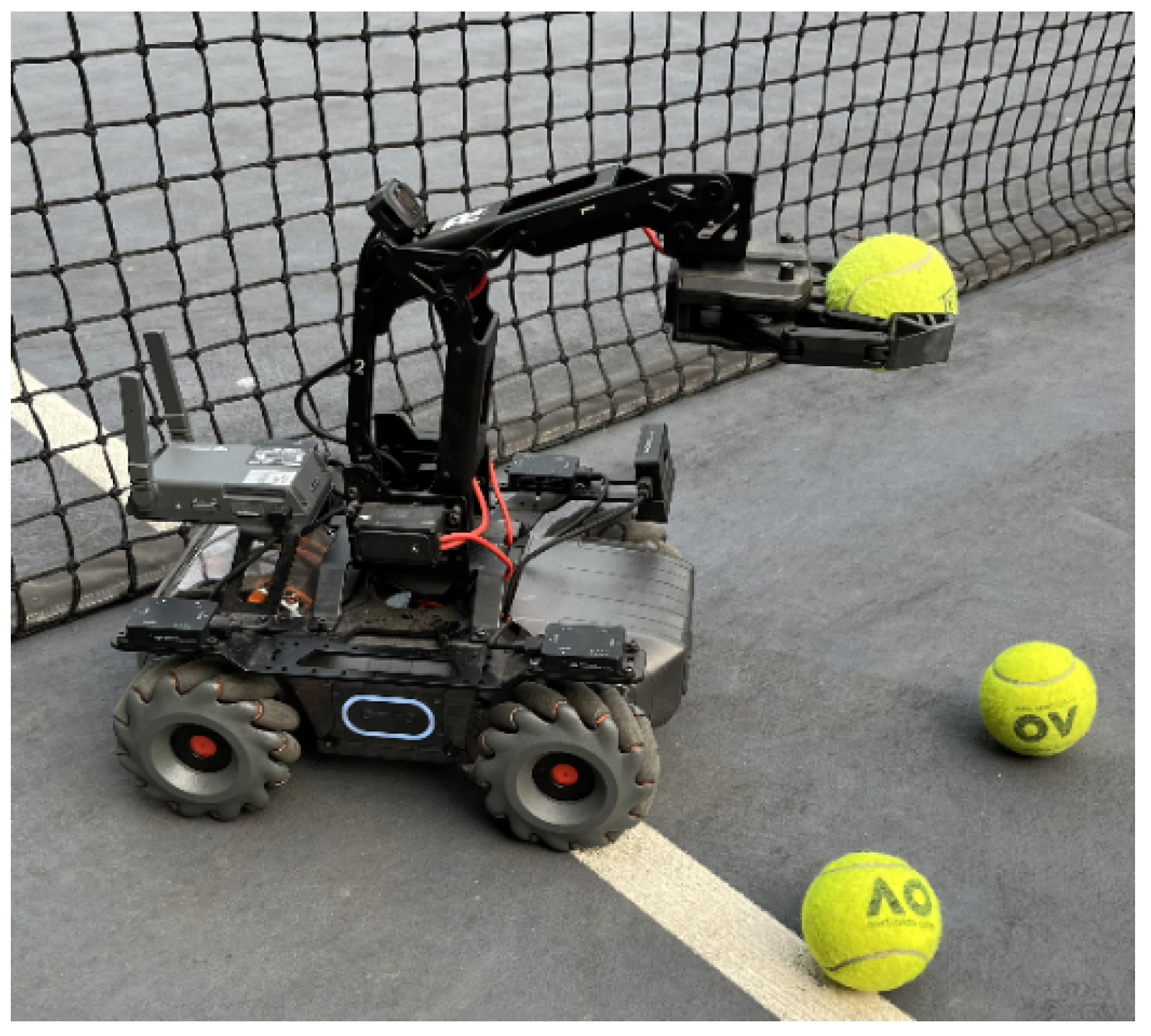
The Robomaster EP is a programming-oriented educational engineering robot from DJI with robust scalability and programmability, as shown in
Figure 1. A parallel robotic arm is used instead of the gimbal structure mounted in the center of the chassis, retaining the image transmission system. A monocular camera is fitted on top of the arm for real-time display and transmission of images, and a mechanical claw is fitted at the end of the arm for more complex tasks. The infrared depth sensor is assembled on top, based on the Time of Flight TOF [
3] principle, through which the sensor emits modulated near-infrared light. After encountering the reflection of an object, the sensor calculates the distance to the object by calculating the time difference or phase difference between the light emission and reflection to achieve intelligent obstacle avoidance [
4] and environment perception [
5], and through the interface call algorithm, real-time detection and identification, improving computational performance. Unlike other tennis ball picking devices, Robomaster EP has a more comprehensive and intelligent overall performance, with the following advantages: (1) The size is small, with a total weight of 3.3 kg, which makes it easy to carry. (2) The range of movement of the robot arm and the opening and closing distance of the robot claw is extensive. The robot arm and claw can be used together to move more flexibly and efficiently. (3) The detection range is more expansive. The infrared depth sensor on top of the arm has a detection range of 0.1–10 m. A monocular camera is mounted on top of the arm to display images in real time. (4) The device has strong scalability and programmability, good compatibility, and it easily calls and deploys algorithms.
For tennis ball detection algorithms, image processing methods are generally used for detection and recognition. For example, the Hough transform [
6] is used to detect tennis balls segmented from video frames by color segmentation. The basic idea is that a tennis ball can be considered a circle from every direction. Any circle can be mapped from an expression under a two-dimensional coordinate system to a three-dimensional space. However, problems include difficulty in feature extraction, susceptibility to the external environment, low detection accuracy, and poor recognition. In addition, Robomaster EP has high requirements for algorithm model parameters and needs to be adapted to lightweight models for easy portability and implementation of algorithms. Traditional deep learning models, such as SSD [
7] and Faster R-CNN [
8], have a large number of model parameters and computation, complex model network structure, difficult deployment, lengthy and costly deployment time, and low performance and detection efficiency of the algorithms, which do not meet the deployment needs of embedded devices. This led to a transition to general-purpose deep learning models, such as the YOLOv5 [
9] algorithm in the YOLO [
10] family of single-stage target detection algorithms, which runs faster and detects quickly for fast detection and identification of tennis balls but has lower detection accuracy compared to two-stage target detection algorithms. Robomaster EP has a more complex model parameter count, computation, and network structure compared to lightweight models. This leads to a more expensive deployment to meet the actual demand. To meet the deployment needs of embedded devices and to improve detection accuracy, Robomaster EP needs to be adapted to the lightweight model to improve efficiency.
According to the existing research, the following three main issues should be considered in a lightweight tennis ball detection algorithm based on Robomaster EP. First, an improved YOLOv5s algorithm is proposed, as the original YOLOv5s algorithm cannot meet the deployment requirements of embedded devices and needs to improve detection accuracy and build lightweight models. Second, the deployment and invocation of the algorithm are implemented through programming for the detection and identification of tennis balls. Thirdly, the detection performance in real scenarios must be verified. An actual tennis court has many tennis balls, as well as the phenomenon of tennis ball occlusion. It is susceptible to weather and light effects, with different scenarios and light intensities leading to different detection results. Using image processing methods, features are challenging to extract, detection accuracy is low, and recognition results could be better. A deep-learning-based tennis ball detection algorithm can improve these problems with better detection performance and robustness in different detection scenarios.
In summary, this study proposes a lightweight tennis ball detection algorithm, YOLOv5s-Z, based on Robomaster EP to achieve accurate detection and recognition of tennis balls. The main work and contributions are as follows: firstly, an improved tennis ball detection algorithm is proposed to construct a lightweight model to improve the detection accuracy while compressing the model and reducing the number of parameters and computation. Secondly, convolutional coordinate attention is incorporated into the Backbone to enhance the ability of the Backbone network to sense the field and capture location information. The original Concat [
11] module in feature fusion is modified into a weighted bidirectional feature pyramid W-BiFPN with settable learning weights to enhance the feature fusion capability and achieve efficient weighted feature fusion and bidirectional cross-scale connectivity, introducing EIOU Loss [
12] and Meta-ACON [
13] to improve the detection accuracy. Finally, the improved algorithm is deployed into Robomaster EP, directly invoked through the interface, and used in real scenarios to detect and identify tennis balls.
3. YOLOv5s-Z
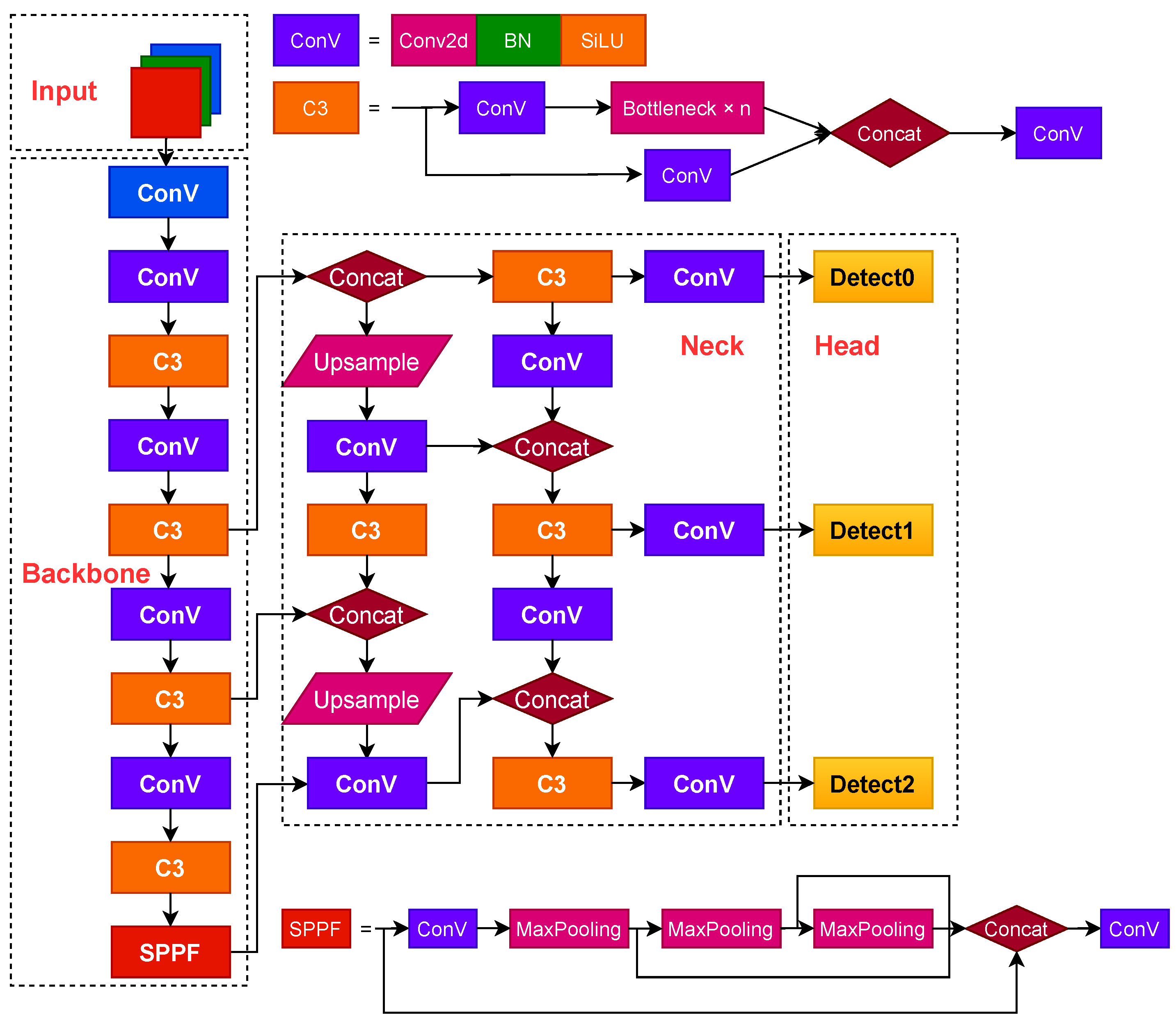
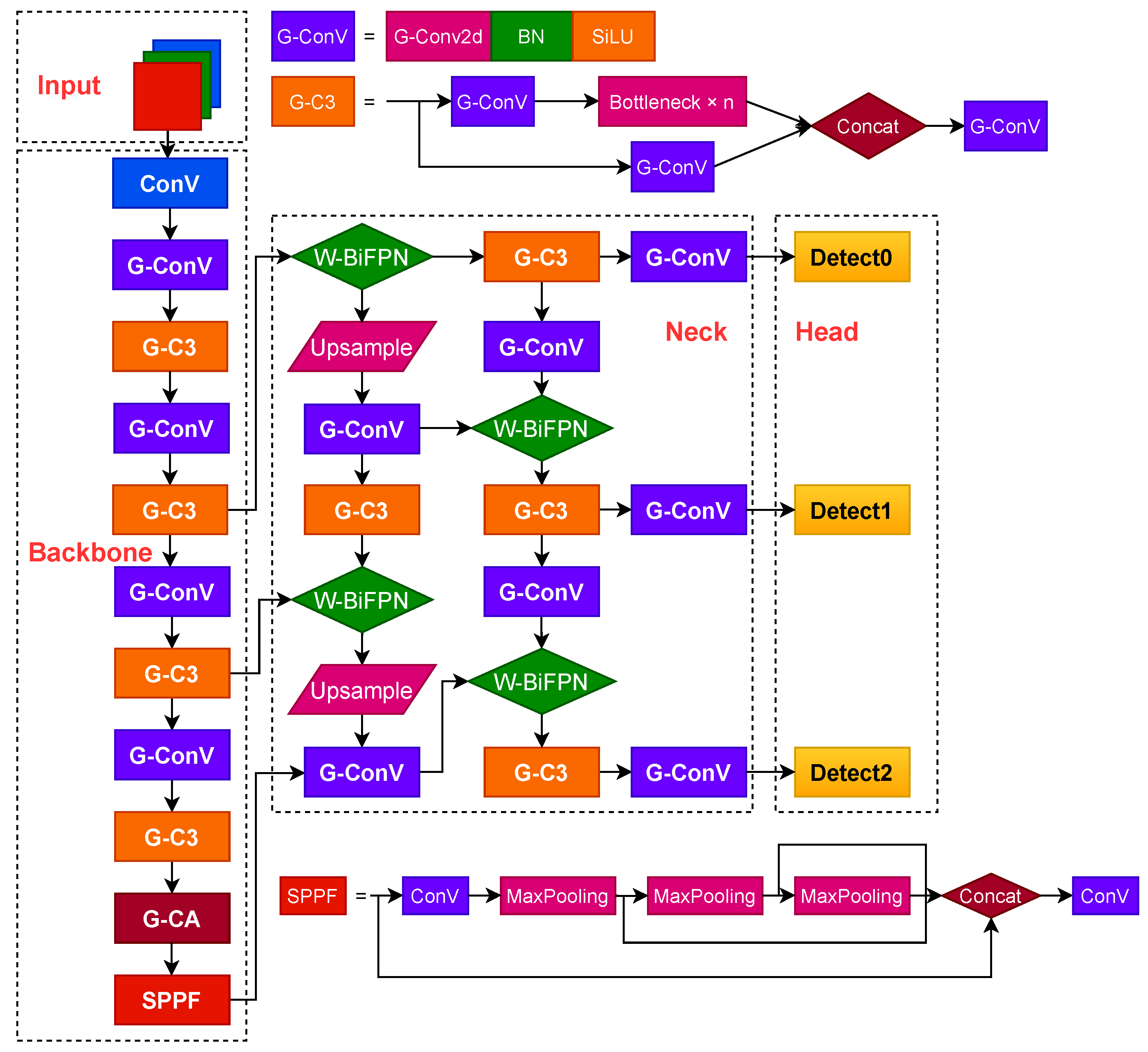
In this study, the network structure is improved and optimized for version 6.1 of the YOLOv5s algorithm, as shown in
Figure 3. It consists mainly of the input, the lightweight G-Backbone and G-Neck network layers, and the output.
3.1. G-Backbone
Based on the lightweight neural network GhostNet, the Conv and C3 modules are subjected to Ghost convolution as well as lightweight processing, and the new G-Conv and G-C3 modules are proposed to build a lightweight G-Backbone, which incorporates the convolutional coordinate attention mechanism G-CA in the G-Backbone to enhance the perceptual field and the ability to capture location information of the Backbone network and better extract the features of the input image. GhostNet is a new end-side neural network architecture proposed by Huawei Noah’s Ark Lab, which builds the lightweight neural network GhostNet by stacking Ghost modules to obtain the Ghost BottleNeck. The structure of the G-Backbone network is shown in
Table 1.
In the above table, Layer denotes the number of layers, From denotes the layer from which the module comes, where −1 denotes the previous layer, Params denotes the number of parameters, Module denotes the module’s name, Arguments denote information about the module, mainly including the number of input channels, output channels, the size of the convolution kernel, and step size information.
For a traditional convolutional neural network, the dimension of the input feature map is c × h × w, where c represents the number of channels, h represents the height of the feature map, and w represents the width of the feature map. The size of the convolutional kernel is c ×
× n, where
k represents the size of the convolutional kernel, and n represents the number of channels of the output feature map. Let the size of the output feature map be h
× w
× n. The total computation is h
× w
× n × c ×
, and the number of parameters is c ×
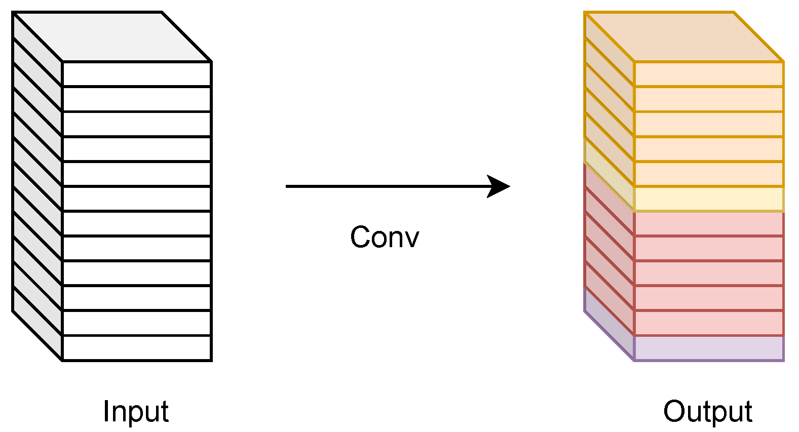
× n. This results in the ordinary output data of convolution Y = X * f + b, where X represents the input data, f represents the c × n convolution operations with a convolution kernel size of
, and b represents the bias term. The process of ordinary convolution is shown in
Figure 4.
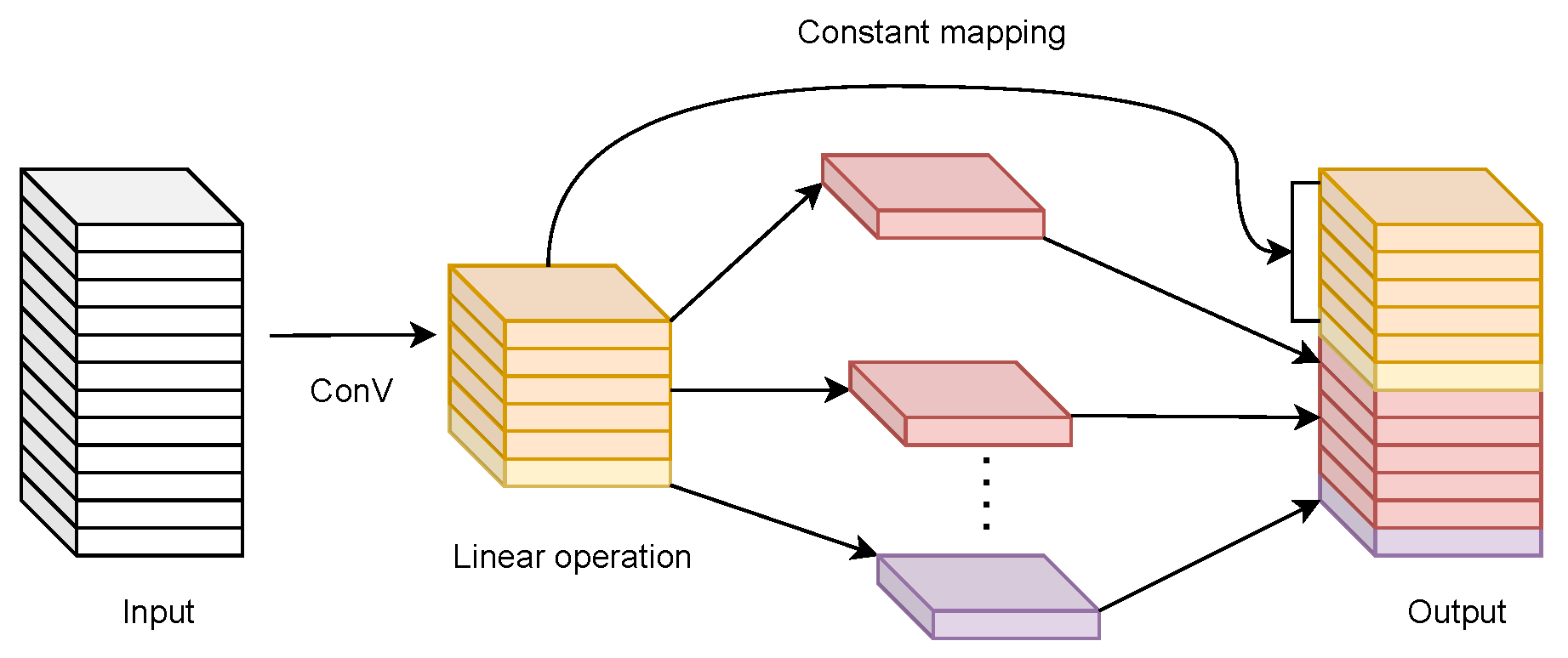
In contrast to ordinary convolution, the process of Ghost convolution is shown in
Figure 5.
The process of Ghost convolution is as follows: first, a small number of feature maps Y
are generated by ordinary convolution, and the feature maps of each channel in the feature maps Y
are used to generate Ghost feature maps
by linear operations. Then, the two sets of different feature maps are stitched together according to the channels. Finally, the same output result as ordinary convolution is obtained. Then, the output data Y
= X ∗ f
+ b of Ghost convolution is calculated as shown in Equation (
1), where
denotes the
j linear operation performed on the
i feature map
generated in the first step of the convolution.
denotes the
i feature map in Y
.
The Ghost module mainly contains a tiny number of convolutions, a constant mapping, and m ×
linear operations, each with an average kernel size of d × d. The formula for the theoretical speed-up ratio of the Ghost module to upgrade the ordinary convolution is shown in Equation (
2).
The formula for the compression ratio of the number of parameters between ordinary convolution and Ghost convolution is shown in Equation (3).
In the above equation, the convolution kernel’s size represents the convolution kernel’s size when linear mapping is performed for each channel. The Backbone provides for better feature extraction of the input images.
Table 2 shows the comparison results between the YOLOv5s model and the YOLOv5s-Ghost model.
As seen from the results in
Table 2, replacing the Ghost module reduces the number of parameters by 48%, the amount of computation by 49%, and the model’s size by 46%. The experimental results demonstrate that the Ghost module achieves a lighter network structure.
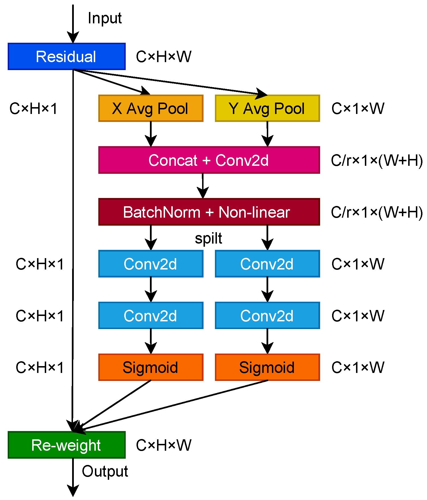
3.2. Convolutional Coordinate Attention
This study proposes a convolutional coordinate attention G-CA, as shown in
Figure 6. By incorporating the convolutional coordinate attention mechanism in the G-Backbone network, the network can obtain location information of a larger area through multiple convolutions, which further enhances the ability of the Backbone network to sense the field and capture location information and enhances the expression ability of the learning features of the mobile network.
Research in neural networks has shown that channel attention significantly improves the model’s performance but ignores some vital location information that facilitates the generation of spatially selective attention maps. Therefore, to alleviate the loss of location information caused by two-dimensional global pooling proposed by attention mechanisms such as SENet [
30] and CBAM [
31], a novel attention mechanism designed for lightweight networks called coordinate attention [
32] was proposed by the National University of Singapore. Compared to channel attention, coordinate attention transforms the feature tensor into individual feature vectors using two-dimensional global pooling, decomposing channel attention into two one-dimensional feature encoding processes that aggregate features along two directions, one of which captures remote dependencies along the spatial direction, and the other retains precise location information along the spatial direction. The resulting feature maps are eventually encoded separately to produce a pair of direction-aware and position-sensitive feature maps that are complementarily applied to the input feature maps and used to enhance the precise localization of targets.
Coordinate attention consists of two main steps: coordinate information embedding and coordinate attention generation. First, given an input feature map X with dimension c × h × w, and using two pooling kernels with spatial ranges (H,1) or (1,W) to encode each channel along the horizontal and vertical coordinates, respectively, the output of the c channel with height h and the c channel with width w is calculated as shown in Equations (4) and (5):
The above two transformations perform feature aggregation along two directions, respectively, and cascade to generate two feature maps, which generate feature maps of spatial information in horizontal and vertical directions f by a convolution operation, which is beneficial to the network for accurate target localization, and the calculation formula is shown in Equation (
6):
After the coordinate information is embedded, the above changes are subjected to the cascade operation, which is a nonlinear activation function that is an intermediate feature map of spatial information encoded along the horizontal and vertical directions, which is decomposed into two tensor sums along the spatial dimension. The transformation operation is then performed using the convolutional transform function, which in turn yields the attention weights of the two spatial directions as
and
, respectively, calculated as shown in Equations (7) and (8):
The
in the above equation is the sigmoid [
33] activation function, and to reduce the complexity and computational overhead of the model, the number of channels is usually reduced using a suitable scaling ratio, and the output is expanded as attention weights, respectively. The final output of the coordinate attention mechanism is obtained, and the calculation formula is shown in Equation (
9):
3.3. G-Neck Network Layer
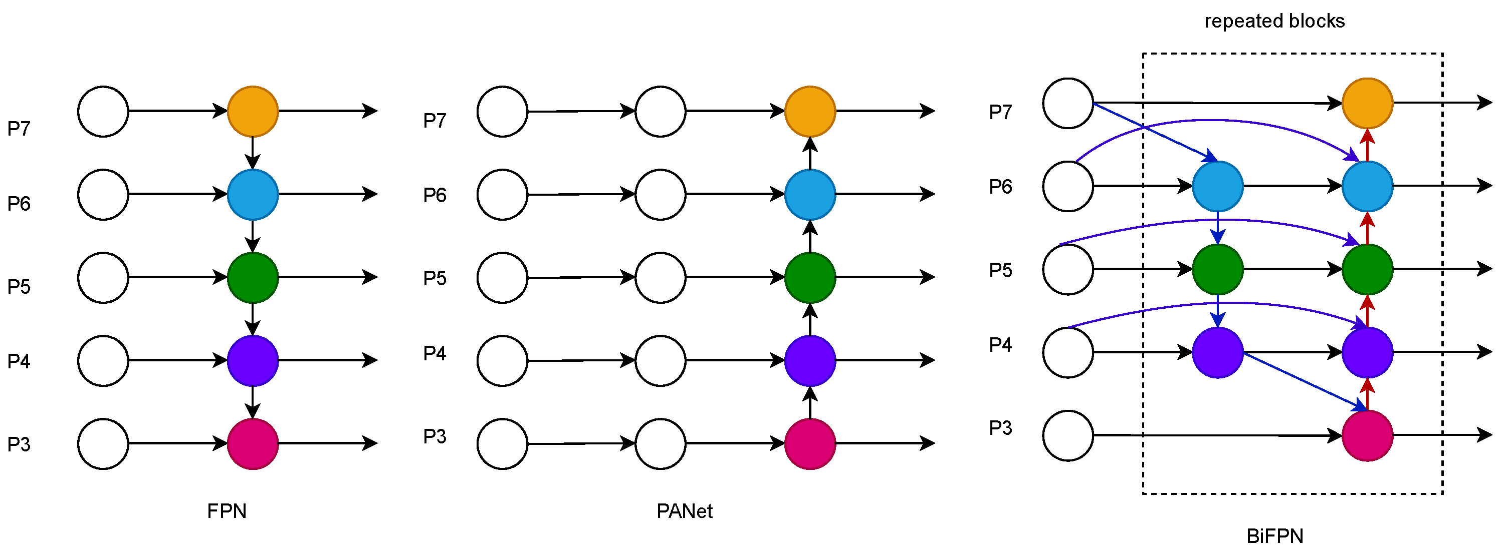
A lightweight G-Neck network layer is constructed, and a weighted bidirectional feature pyramid W-BiFPN with settable learning weights is proposed to be incorporated into the G-Neck network layer. Based on the weighted bidirectional feature pyramid BiFPN, a settable learning weight coefficient W is set to strengthen the feature fusion capability further and improve the detection speed to achieve more efficient weighted bidirectional feature fusion, which is more convenient for the network to extract features.
Figure 7 shows the development process of Neck networks in recent years, starting with the top-down unidirectional fusion FPN feature pyramid structure, which establishes a top-down pathway for feature fusion and uses feature maps for prediction, which can improve accuracy to a certain extent but will be limited by the one-way information flow. The network structure of PANet [
34] for bidirectional fusion adds to the FPN [
35], a bottom-up path aggregation network. The main idea is that the higher-level feature maps have more vital semantic information for object classification. In comparison, the bottom-level feature maps have more vital positional information for object localization. PANet network passes the positional information from the bottom-level layer to the prediction feature layer, making the prediction feature layer have higher semantic information and positional information, which is more conducive to target detection and thus improves detection accuracy. The PANet network structure also has Adaptive feature pooling, and complete connection fusion is proposed in the PANet network structure. Adaptive feature pooling is used to aggregate features between different layers to ensure the integrity and diversity of features, and complete connection fusion is used to obtain an accurate prediction layer. The main idea of the weighted bidirectional feature pyramid network structure BiFPN [
36] is compelling bidirectional cross-connections and weighted feature fusion and top-down feature fusion followed by bottom-up feature fusion. Multi-scale feature fusion is the aggregation of features at different resolutions.
Different input features have different resolutions, so the contribution to the output features is uneven. To solve the problem, an additional weight is added to each input so that the network learns the importance of each input feature; biFPN uses a fast normalized weighted fusion method, calculated as shown in Equation (
10):
where
is achieved by adding the ReLU activation function after each
, the weights are divided by the weighted sum of all values to achieve the normalization operation, and the value of each normalization weight is between zero and one. BiFPN integrates bidirectional cross-scale connectivity and fast normalized fusion, and the computational equations of the fusion feature process are shown in Equations (11) and (12) for BiFPN at Level 6 nodes.
In the above equation, denotes the intermediate features of the sixth layer in the top-down path, and denotes the output features of the sixth layer in the bottom-up path. To improve efficiency, feature fusion is performed using depth-separable convolution, and batch normalization and activation functions are added after each convolution, where Resize is the upsampling or downsampling operation, and w is the learned parameter to distinguish the importance of different features in the feature fusion process.
3.4. EIOU Loss
The default Loss function in YOLOv5s is CIOU Loss [
37], and the formula for CIOU is shown in Equation (
13). The aspect ratio of the regression frame is considered in the Loss function based on DIOU Loss [
38]. The loss of the detection frame scale and the loss of the length and width are added to make the prediction frame more realistic and further improve the regression accuracy. The DIOU calculation formula is shown in Equation (
14). The disadvantage is that the aspect ratio needs to be more specific, and the balance of complex and easy samples is not considered. In this study, EIOU Loss is introduced, and the formula of EIOU Loss is shown in Equation (
15). Based on the penalty term of CIOU Loss, the aspectual influence factors of the prediction frame and the rear frame are split. The length and width of the prediction and the rear frames are calculated separately to solve the problems in CIOU Loss.
In the above equation, b and denote the centroids of the prediction frame and the actual frame, respectively, denotes the Euclidean distance calculated between the two centroids, and c denotes the diagonal distance of the minimum closed region containing both the prediction frame and the actual frame. We can see that the Loss consists of three main components: the overlap loss between the predicted frame and the real frame , the center distance loss between the predicted frame and the real frame , and the width and height loss between the predicted frame and the real frame . and continue the method in , and the width and height loss directly makes the difference between the width and height of the predicted frame, and the real frame minimizes the difference between the width and height of the predicted frame and the rear frame, which makes the convergence faster.
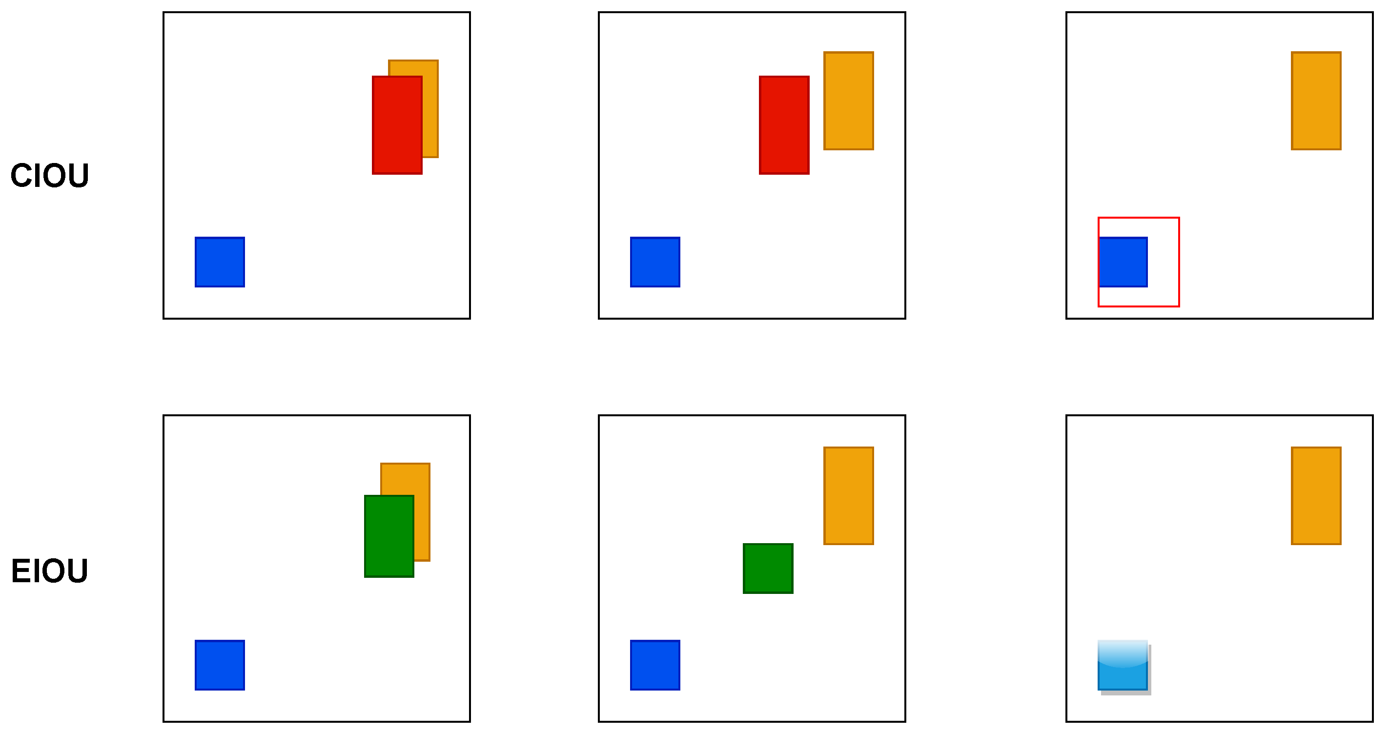
The comparison diagram of the iterative process of CIOU and EIOU Loss prediction frames is shown in
Figure 8. The red and green boxes represent the regression process of CIOU and DIOU prediction frames, the blue box is the actual frame, and the yellow box is the pre-defined anchor frame. The comparison chart shows that the width and height of EIOU can be increased or decreased at the same time, but not CIOU. In general, EIOU outperforms CIOU, so this study introduces EIOU Loss as the Loss function.
3.5. Meta-ACON Activation Function
The default activation function in YOLOv5s is ReLU [
39], which is the most common activation function, mainly because of its non-saturation and sparsity properties, with the disadvantage that it can have the severe consequence of neuronal necrosis. ReLU is essentially a function and is calculated as shown in Equation (
16):
Consider the n values of the standard maximum function MAX, whose smoothness and differentiability are approximated by
, calculated as shown in Equation (
17):
where
is a connection coefficient, and
tends to the maximum when
tends to infinity, and
tends to the arithmetic mean when
tends to zero. In neural networks, the common activation function is expressed in the form of
, where
and
are linear functions.
The Swish [
40] activation function, obtained by the NAS [
41] search technique, is an approximate smoothing of the ReLU activation function. The general form of Swish’s ACON activation function is obtained by analyzing the general form of the Maxout [
42] series of activation functions of ReLU. The ACON generalization yields ACON-A, ACON-B, ACON-C, the Meta-ACON, and other variant forms. This study introduces Meta-ACON, which adaptively selects whether or not to activate neurons and introduces a switching factor to learn the parameter switching between nonlinear activation and linear non-activation to improve the detection accuracy of the algorithm.
4. Experimental Results
4.1. Experimental Environment
This experiment was based on the Pytorch 1.11.0 framework, CUDA version 11.5, and conducted on the PyCharm platform, and the model training was accelerated by GPU. The specific experimental environment parameters were configured as shown in
Table 3.
4.2. Datasets
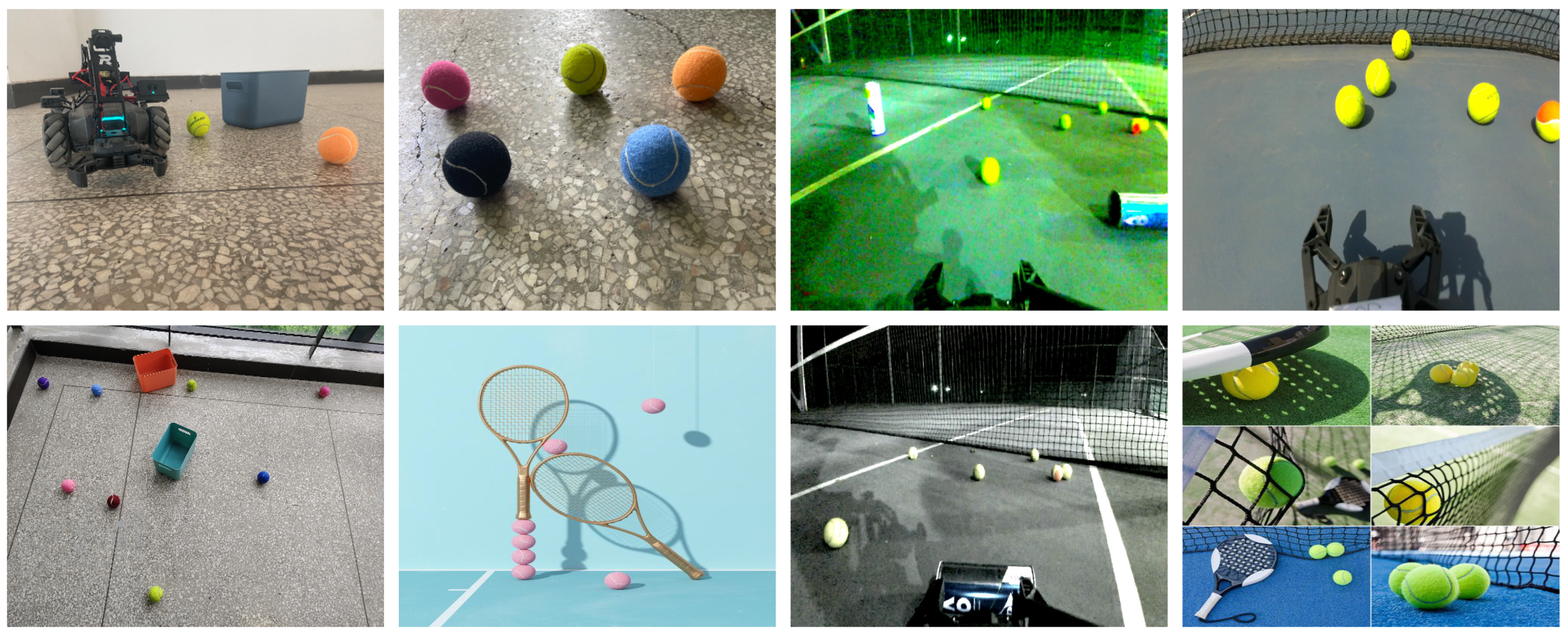
In this study, 1180 homemade tennis ball datasets were used. The sources of the datasets included tennis ball pictures taken by the monocular camera fitted with Robomaster EP, tennis ball pictures taken by mobile phones, and tennis ball pictures obtained by crawlers, containing different colors, different scenes, and different time tennis ball pictures to ensure the diversity of the datasets. The specific information is shown in
Table 4.
The dataset was normatively annotated with explicit annotation using Make Sense. At the same time, the training set, validation set, and test set were divided according to 8:1:1. Before training the model, some of the datasets were pre-processed, including randomly increasing or decreasing the brightness and contrast of the images, and combined with the Mosaic data enhancement method that comes with YOLOv5 to enrich the datasets and enhance the generalization ability of the model and the robustness of the validation model.
Figure 9 shows an example graph representing the dataset.
4.3. Training Strategy and Evaluation Index
All models were trained from scratch using the same training strategy and parameters, hyperparameter profiles, and pre-warm training parameters, all without pre-training weights. The parameters were updated iteratively using the SGD optimizer with an initial learning rate of 0.01, a momentum parameter of 0.937, and a batch size of 16. The warm-up method with an epoch of 3 and a momentum parameter of 0.8 was used to warm up the learning rate, and all models were trained for 300 rounds.
In this study, the model was evaluated using evaluation metrics including
[email protected], Recall, Parameters, GFLOPs, and Weight. Here,
[email protected] represents the average AP at the IOU threshold of 0.5, which is used to reflect the recognition ability of the model. Recall represents the ratio of correctly detected positive samples to all positive samples, Parameters represent the number of parameters of the model, and GFLOPs represent the number of floating point operations performed by the model. Parameters and GFLOPs are important indicators of the model algorithm, which measure the complexity of the model in the dimensions of time and space, respectively. The calculation equations are shown in Equations (18)–(21).
where n represents the number of categories, p represents precision, R represents recall, P(R) represents the precision and recall curves, TP represents the number of detection frames with IOU ≥ set threshold, FP represents the number of detection frames with IOU ≤ set threshold, and FN represents the number of missed targets.
4.4. Comparative Experimental Results and Analysis
To verify the effectiveness of the improved algorithm, commonly used target detection algorithms were selected for comparative analysis, and the same training strategy and parameters were used for each group of experiments. The experimental results are shown in
Table 5.
From the results of the comparison experiments, it can be seen that the algorithm proposed in this study had the most comprehensive performance, taking into account the needs of lightweight models and detection accuracy, with solid generalization ability, the highest mean accuracy and recall, and slightly more parameters, computation, and model size than the lightweight neural networks Mobilenet and Shufflenet, but Mobilenet and Shufflenet had lower mean precision and recall. Compared to the original YOLOv5s algorithm, the number of parameters and computation were reduced by 42% and 44%, respectively, the model size was reduced by 39%, and the average precision improved by 2%, verifying the effectiveness of the improved algorithm. Compared with the classical target detection algorithms SSD and Faster R-CNN, the overall performance was much better, with a significant increase in mean accuracy and recall and a significant reduction in the number of parameters, computation, and model size. The performance of the YOLO family of target detection algorithms, YOLOv3, YOLOv4, YOLOX, and the lightweight model, was still much better. Even when compared to the current best-performing YOLOv7 algorithm, the proposed algorithm has better overall performance, reducing the number of parameters and computation by 32% and 33%, respectively, and the model size by 25% compared to YOLOv7-tiny, validating the effectiveness of the improved algorithm and the lightness of the model.
4.5. Ablation Experimental Results and Analysis
To verify the feasibility of the improvement module, six sets of ablation experiments were designed based on YOLOv5s. The same training strategy was used for each set of experiments. The results of the ablation experiments are shown in
Table 6. Where improvement point 1 indicates the introduction of the lightweight G-Backbone, improvement point 2 indicates the addition of the G-CA attention mechanism, improvement point 3 indicates the addition of the W-BiFPN module, improvement point 4 indicates the introduction of EIOU Loss, and improvement point 5 indicates the introduction of the Meta-ACON activation function.
From the results of the ablation experiments, the introduction of G-Backbone significantly reduced the number of parameters, computation, and model size of the network structure. At the same time, the average precision means value remained stable, verifying the effectiveness of the lightweight module. With the introduction of G-CA and W-BiFPN, although the number of parameters and computational effort increased slightly, the mean accuracy and recall rate increased, which verified the effectiveness of the improved module. With the introduction of EIOU Loss, the number of parameters, computation volume, and model size remained unchanged. However, the average precision means value increased slightly, and the recall rate increased by nearly 7%, verifying that the introduction of EIOU Loss outperforms CIOU Loss and improves the detection accuracy. With the introduction of Meta-ACON, although the number of parameters, computation, and model size increased slightly, the mean accuracy and recall rate increased, verifying the effectiveness of the improvement. By incorporating all the improved modules in this paper, the number of parameters, computation, and model size was reduced. The mean accuracy and recall rate increased by 2% and 7%, respectively, which combines the lightweight model and detection accuracy.
4.6. Case Study
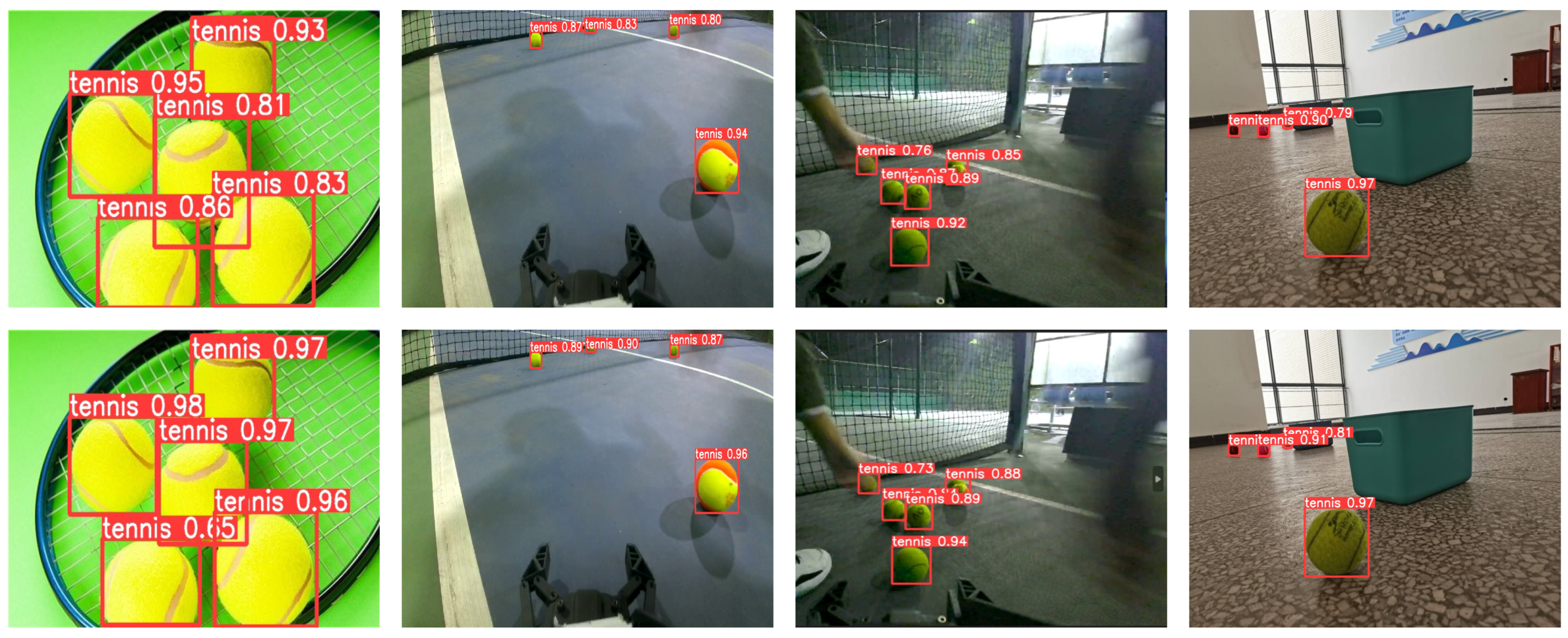
We further empirically investigated the detection performance in different scenarios. The detection results are shown in
Figure 10, all based on real detection scenarios. The top row indicates the detection results of the YOLOv5s algorithm, and the bottom row indicates the detection results of the YOLOv5s-Z algorithm. The detection scenarios are a tennis racket on the ground, a tennis court in the morning, a tennis court in the evening, and an aisle outside the laboratory. Overall, the detection accuracy of the YOLOv5s-Z algorithm was higher than that of the YOLOv5s algorithm, regardless of the different scenes or periods of the same scene.


