Vehicle Distance Measurement Method of Two-Way Two-Lane Roads Based on Monocular Vision

Abstract

The longitudinal distance between the vehicle and the forward vehicle, as well as the longitudinal distance between the vehicle and the opposite vehicle, is the main risk factor of overtaking behavior on two-way two-lane roads. Accurate measurement of these distances is the basis and key to automatic driving technology of two-way two-lane roads. In order to measure these longitudinal distances and improve the ranging accuracy, a vehicle distance measurement method of two-way two-lane roads based on monocular vision was proposed. Firstly, the vehicle detection model suitable for two-way two-lane roads was trained using YOLOv5s neural network. Secondly, aiming at the problem that the camera roll angle is not considered in the traditional geometric ranging method, the influence of the roll angle of the camera on ranging results using the traditional geometric ranging method was analyzed. In addition, the improved geometric ranging method considering the roll angle of the camera was proposed. Then, tests were conducted on a two-way two-lane road, and the results showed that the proposed method was effective. Compared with other methods, the improved geometric ranging method has higher ranging accuracy in this scene and can provide a reference for vision-based vehicle distance measurement in multi-lane scenes.

1. Introduction

As one of the most common highway forms in China’s highway network, two-way two-lane roads account for more than 95% of the total highway mileage in the western region and play an important role in the highway network [1]. Due to the particularity of two-way two-lane roads, vehicles need to borrow the opposite lane when overtaking, which is common in many developing countries in Asia, such as Vietnam and China [2]. However, a serious traffic accident may occur because of the false temporal and distance estimations regarding the oncoming vehicles made by drivers when the vehicle is overtaking [3,4,5,6]. Therefore, improving the driving safety of vehicles on two-way two-lane roads is an important research content of advanced driving assistance systems. Moreover, automatic driving technology of two-way two-lane roads will be an important research direction in the future. Research shows that the longitudinal distance between the vehicle and the forward vehicle, as well as the longitudinal distance between the vehicle and the opposite vehicle, is the main risk factor of overtaking behavior on two-way two-lane roads [7]. Therefore, measuring these distances is the basis and key to the automatic driving technology of two-way two-lane roads.

The primary task of vehicle distance measurement is vehicle detection. With the rapid development of computer vision, vehicle detection and distance measurement technology based on on-board cameras has been improved and promoted. Among them, the monocular vision system has attracted the attention of the industry because of its simple structure, small amount of calculation, and high real-time performance [8].

In terms of vehicle detection technology based on computer vision, the traditional vehicle detection method uses prior knowledge, such as vehicle color and edge, to detect the vehicles in front. However, due to its dependence on prior knowledge, the method has insufficient adaptability and generalization capabilities [9]. The vehicle detection method based on deep learning extracts vehicle features through the convolutional neural network, which has stronger adaptability, greatly improves detection accuracy and speed, and is more widely used [10].

In terms of vehicle distance measurement technology, at present, vision-based vehicle ranging methods include: the geometric relationship method, imaging model method, data regression modeling method, inverse perspective mapping method, and image depth estimation based on deep learning. Shen Z [11] used the relationship between the distance and height of the target in the image to establish a mathematical regression model and then used the quadratic curve to measure the distance of the regression model. This method has a large workload and lacks the generalization ability and portability of the model. Bao D [12] used the vehicle width ratio to measure the distance. This method is easily affected by the diversity of vehicle size and thus affects the ranging accuracy. Tuohy S and Adamshuk R [13,14] converted the original image into an aerial view to restore the plane information of the road ahead. The IPM image obtained through the conversion is used to calculate the distance of the target vehicle. This method is simple and feasible but ignores the influence of the camera attitude angle. Ding M [15] used a deep learning network to train a large number of depth maps, then combined the estimated depth map with the results of instance segmentation to measure the distance between the subject vehicle and the target vehicle. This method has high-ranging accuracy, but the data contain more redundant information, which is not easy to be processed. The geometric relationship method establishes the ranging model through the geometric relationship between the camera and the target in a three-dimensional coordinate system; it has a small workload, a simple model, and portability compared with other methods. Therefore, this paper selected the geometric relationship method to complete the distance measurement task of vehicles on two-way and two-lane roads. Numerous researchers have conducted in-depth research on this method. Stein G [16] proposed the basic model of the geometric ranging method and discussed the influence of pixel error on ranging accuracy. In order to improve ranging accuracy, Liu C and Rezaei M [17,18] considered the influence of the pitch angle of the camera on ranging and established a traditional geometric ranging method considering the pitch angle of the camera. Since then, many research and practical applications have been completed with the support of this method [19,20,21,22,23]. Although the above research on vehicle distance measurement methods based on geometric relationships has achieved good results, the influence of the roll angle caused by camera rotation around its optical axis on this method has been ignored.

In order to measure the longitudinal distance between the vehicle and the forward vehicle, as well as the longitudinal distance between the vehicle and the opposite vehicle, on the two-way two-lane roads, and improve the ranging accuracy, the main contributions of this paper are as follows:

• The vehicle detection model suitable for two-way two-lane roads was trained.
• The influence of the roll angle of the camera on ranging results using the traditional geometric ranging method was analyzed. When the roll angle of the camera exists, the ranging result will deviate from the normal value. The degree of deviation will vary with the vehicle positions. Moreover, the larger the roll angle, the greater the deviation.
• The improved geometric ranging method considering the roll angle of the camera was proposed. Through experimental verification and method comparison, the proposed method is effective, and the improved geometric ranging method has higher ranging accuracy than the other two methods on two-way two-lane roads.

2. Methods

The overall framework of this paper is shown in Figure 1. Firstly, a data set of traffic flow of two-way two-lane roads was established, and the vehicles in the data set were classified as forward or opposite vehicles. Secondly, a vehicle detection model of two-way two-lane roads was trained by using YOLOv5s neural network to detect the forward and opposite vehicles and calculate the feature points of vehicles. After that, the rotation model of the imaging plane of the camera will be established. The simulation test was designed to analyze the influence of the roll angle of the camera on ranging results using the traditional geometric ranging method, and the improved geometric ranging method considering the roll angle of the camera was proposed. The feature point of the vehicle and parameters of the camera were used as the input of the vehicle distance measurement model, and the model output the vehicle category and the longitudinal distance between the vehicle and the forward vehicle, as well as the longitudinal distance between the vehicle and the opposite vehicle. Finally, an experiment with actual vehicles carried out on the actual two-way two-lane roads was designed and compared with other methods to verify the feasibility and ranging accuracy of this method.

2.1. Establishment of Vehicle Detection Model of Two-Way Two-Lane Roads

2.1.1. Collection and Labeling of Data Set

In order to train the vehicle detection model suitable for two-way two-lane roads, this paper used the traffic flow atlas of the real two-way two-lane roads as the data set. The total number of samples in the data set is 5516, including 3925 traffic flow pictures of urban and rural two-way two-lane roads taken from the BDD100K public data set and 1591 self-made traffic flow pictures of on-campus two-way two-lane roads. Each sample contains at least one forward vehicle and one opposite vehicle. Partial samples of the data set are shown in Figure 2a. The open-source image labeling tool LabelImg was used to manually label the samples; each vehicle was labeled with a rectangular box, and a tag file in TXT data format was generated. The tag file included the file name of the sample, the category, the coordinates of the rectangular box, the length and width of the rectangular box, and other information. In this paper, the object categories were forward vehicles and opposite vehicles. According to the driving characteristics of the vehicles on two-way two-lane roads, the vehicle showing its back was labeled as ‘back’, and the vehicle showing its front was labeled as ‘front’. A total of 13,774 vehicles were labeled, 7832 of which were forward vehicles and 5942 of which were opposite vehicles. Examples of labeling are shown in Figure 2b.

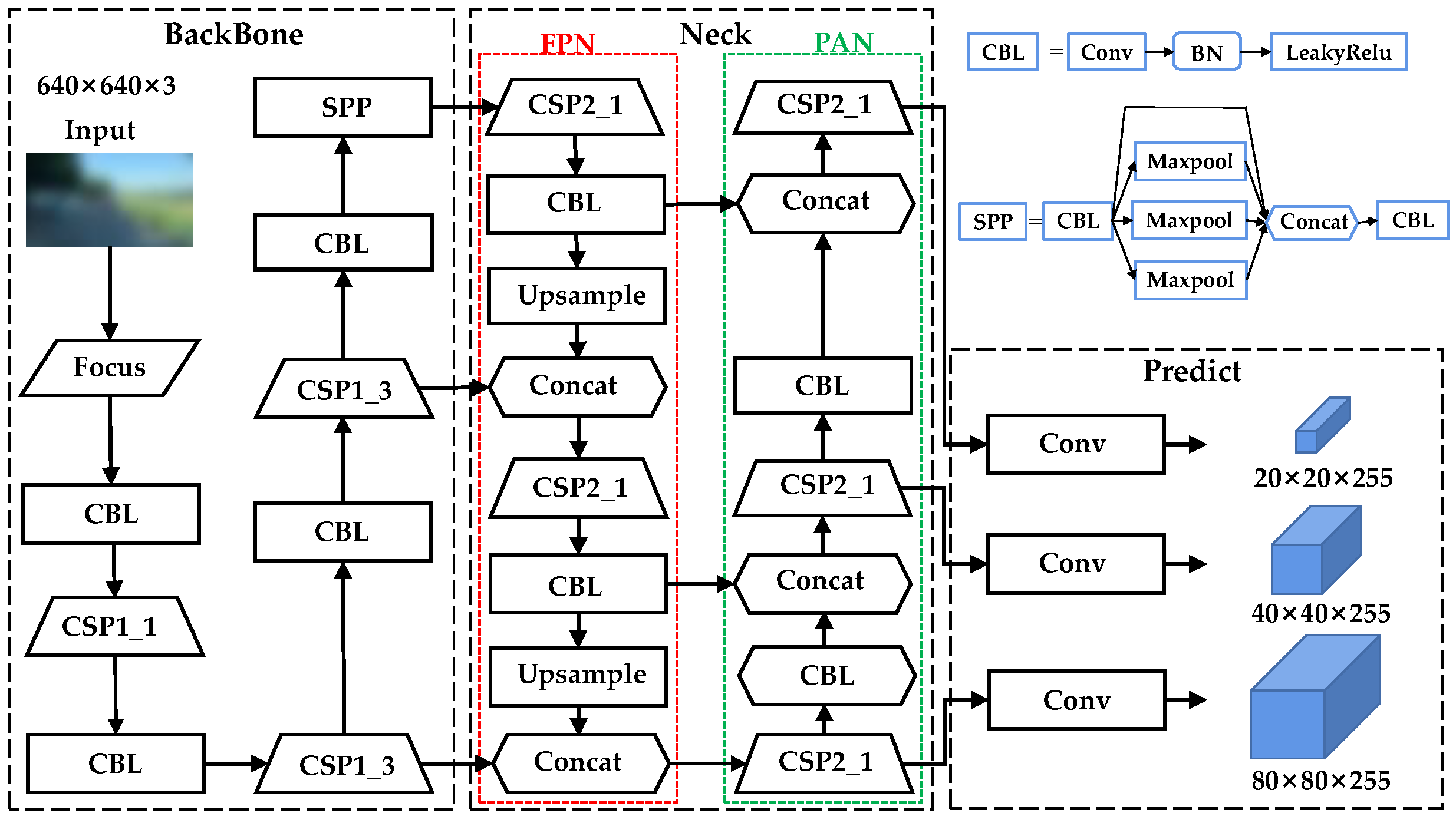
2.1.2. Training of Vehicle Detection Model Using YOLOv5s Network

YOLOv5 is the fifth generation YOLO (you only look once) series of target detection methods proposed in 2020 and is the most advanced detection network in this series of algorithms [24]. Compared with other algorithms in the YOLO series, YOLOv5 has a smaller model size and faster training and image-processing speed. YOLOv5 has four network scales: s, m, l, and x. In addition, YOLOv5s has the smallest network depth and fast detection speed. Therefore, this paper selected the YOLOv5s network to train the vehicle detection model of two-way two-lane roads. The network structure of YOLOv5s is divided into four parts: input, backbone, neck, and prediction. Its network structure is shown in Figure 3.

The basic component of the network is CBL, which is composed of a convolution layer (Conv), batch normalization layer (batch normalization, BN), and activation function (Leaky ReLU). At the input of the network, images are preprocessed, and the mosaic data enhancement method is used to randomly scale, cut, arrange, and then splice them to improve the detection effect of small targets. In addition, the adaptive anchor box calculation function is also applied to adaptively calculate the value of the optimal anchor box in different training sets during each training [25]. The backbone network is used to extract image features. First, the Focus structure is used to slice images to reduce the number of network layers, effectively alleviating the problem of gradient disappearance [26]. The input image of 640 × 640 × 3 first becomes a feature map of 320 × 320 × 12 after the slicing operation, and it finally becomes a feature map of 320 × 320 × 32 after a convolution operation of 32 convolution kernels. Then, referring to the design idea of the cross-stage partial network (CSP Net), two kinds of CSP structures corresponding to CSP1_X in the backbone and CSP2_X in the neck are designed to optimize the problem of excessive computation caused by repeated gradient information [27]. These CSP structures divide the feature map of the basic layer into two branches for convolution operation and finally use the Concat function to merge the two branches. At the end of the backbone network, the spatial pyramid pooling networks (SPP Net) are applied; they realize the fusion of local features and global features by using three parallel max pooling layers (Maxpool) to down-sample the feature map. The neck is used to further improve the ability of feature extraction; it combines the two structures of the feature pyramid network (FPN), which conveys the high-level feature information in a top-to-bottom manner, and the path aggregation network (PAN), which conveys strong positioning characteristics in a bottom-to-top manner to realize the fusion of features of different scales and enable the model to obtain richer feature information. In the prediction layer, the optimal target frame is filtered by combining the loss function GIOU and the non-maximum suppression (NMS) algorithm [28].

In order to evaluate the performance of the trained model, precision (P), recall (R), average precision (AP), and mean average precision (mAP) were used as evaluation indicators. P represents the proportion of the number of targets correctly detected to the number of all targets detected. R represents the proportion of the number of targets correctly detected to the number of all actual targets. They were respectively defined as follows [29]:

$$P=\frac{TP}{TP+FP}\times 100\%,$$

(1)

$$R=\frac{TP}{TP+FN}\times 100\%,$$

(2)

where TP represents the number of targets that are correctly detected, FP represents the number of non-targets that are detected as targets, and FN represents the number of targets that are detected as non-targets.

The experimental data can be used to draw the PR curve of the model. The area enclosed by the curve is AP, which is used to evaluate the model’s detection performance for a single category of targets. Variable mAP is the average value of AP; the value of mAP is between 0–1. The closer the mAP value is to 1, the better the model performance and the stronger the detection capability. They were respectively defined as follows [29]:

$$AP={\displaystyle {\int }_0^{1}P\left(R\right)dR,}$$

(3)

$$mAP=\frac{{\displaystyle {\sum }_{i=1}^{N}A{P}_i}}{N}.$$

(4)

where N represents the number of categories.

2.2. Establishment of Vehicle Distance Measurement Model

2.2.1. Imaging Principle of Monocular Vision

The imaging principle of the monocular vision system can be described by the pinhole imaging model. The imaging process is actually the process of mapping the three-dimensional space scene in reality to the two-dimensional space. Four coordinate systems can be used to express this mapping relationship. As shown in Figure 4, P is the three-dimensional coordinate point, and P’ is the imaging position of Pon, the image plane of the camera.

As shown in the above figure, UO₀V is the pixel coordinate system, which takes O₀ of the CCD image plane as the coordinate origin. The U-axis and V-axis are respectively parallel to the two vertical edges of the CCD image plane, and the coordinates are represented by (u, v). XO₁Y is the image coordinate system, which takes the center of the CCD image plane as the coordinate origin O₁, the X-axis and Y-axis are the axes parallel to the U-axis and V-axis of the pixel coordinate system, respectively, and (u₀, v₀) is the position of O₁ in the pixel coordinate.

O_wX_wY_wZ_w is the world coordinate system, which is the absolute coordinate system of the objective world, and the coordinates are represented by (X_w, Y_w, Z_w). O_cX_cY_cZ_c is the camera coordinate system, which takes the optical center of the camera as the coordinate origin O_c; the X_c-axis and the Y_c-axis are the axes parallel to the X-axis and Y-axis of the image coordinate system, respectively, and Z_c is the optical axis of the camera. The world coordinate system can be converted into the camera coordinate system through the rotation matrix R and translation matrix T.

Setting dx and dy as the physical conversion scale of the unit pixel in the X and Y directions in the image coordinate system, respectively, and f as the distance between the origin of the image coordinate system and the origin of the camera coordinate system, that is, the focal length. The conversion formula between the coordinates of the three-dimensional world coordinate system and the coordinates of the two-dimensional pixel coordinate system is as follows [30]:

$$\begin{array}{l}{Z}_c\left[\begin{array}{c}u\\ v\\ 1\end{array}\right]=\left[\begin{array}{ccc}1/dy& 0& u_0\\ 0& 1/dy& v_0\\ 0& 0& 1\end{array}\right]\left[\begin{array}{cc}\begin{array}{ccc}f& 0& 0\\ 0& f& 0\\ 0& 0& 1\end{array}& \begin{array}{c}0\\ 0\\ 0\end{array}\end{array}\right]\left[\begin{array}{cc}R& T\\ \overrightarrow{0}& 1\end{array}\right]\left[\begin{array}{c}{X}_w\\ Y_w\\ Z_w\\ 1\end{array}\right],\\ =\left[\begin{array}{cc}\begin{array}{ccc}{a}_x& 0& u_0\\ 0& a_y& v_0\\ 0& 0& 1\end{array}& \begin{array}{c}0\\ 0\\ 0\end{array}\end{array}\right]\left[\begin{array}{cc}R& T\\ \overrightarrow{0}& 1\end{array}\right]\left[\begin{array}{c}{X}_w\\ Y_w\\ Z_w\\ 1\end{array}\right]\end{array}$$

(5)

where a_x = f/dx, a_y = f/dy.

2.2.2. Calculation of Feature Point of Vehicle

The midpoint of the bottom edge of the vehicle detection frame output from the two-way two-lane vehicle detection model is selected as the feature point of the vehicle, and it is input into the vehicle distance measurement model to calculate the distance between vehicles.

The pixel coordinates of the vehicle detection frame output from the vehicle detection model are: the upper left corner (u₁, v₁) and the lower right corner (u₂, v₂). In addition, (u_c, v_c) is the coordinate of the midpoint at the bottom of the detection frame and also the pixel coordinates of the feature point of the vehicle. It can be obtained from Equation (6):

$$\{\begin{array}{c}{u}_c=\left(u_1+u_2\right)/2\\ v_c=v_2\end{array}.$$

(6)

2.2.3. Traditional Geometric Ranging Method

The traditional geometric ranging method calculates the distance between two vehicles by establishing the geometric relationship between the position of the feature point of the front vehicle on the image plane of the on-board camera and the position of the feature point of the front vehicle in the three-dimensional space. The pitch angle of the camera, that is, the angle between the optical axis of the camera and the horizontal road surface, was taken into account when establishing the model. The model structure is shown in Figure 5.

In the above figure, P is the feature point of the front vehicle; O is the optical center of the camera; AB is the image plane of the camera; C is the center point of the image plane, and its pixel coordinate is (u₀, v₀); P’ is the imaging position of P in the camera image plane, and its pixel coordinate is (u_p, v_p). CF is the optical axis of the camera; D is the projection point of the camera on the horizontal ground; G and E are the intersections of the upper edge of the camera image and the ground, and the intersection of the lower edge of the camera image and the ground, respectively; K is the projection point of the front end of the vehicle body on the horizontal ground; l is the longitudinal distance between the camera and the head of the vehicle; h is the height of the camera from the ground; f is the focal length in the pixel; α is the angle between the camera optical axis and the horizontal road surface, that is, the pitch angle of the camera.

According to the geometric relationship, the formula for calculating the longitudinal distance d between two vehicles can be obtained:

$$d=h\times \tan {\displaystyle (}\left(90-\alpha \right)-\left(\arctan \left(\left(v_p-v_0\right)/f\right)\right){\displaystyle )}-l.$$

(7)

2.2.4. Improved Geometric Ranging Method

Although the traditional geometric ranging method is simple and easy to implement, it only considers the pitch angle of the camera and ignores the roll angle of the camera, that is, the angle between the Y axis of the camera’s imaging plane and the vertical line of the ground. However, the manual installation will inevitably lead to camera inclination in multiple dimensions, so the traditional geometric ranging method cannot meet the actual situation. It can be seen from Equation (7) that the distance d is related to the position of the feature point of the vehicle on the imaging plane. Therefore, a model of the camera’s imaging plane when the camera has a roll angle is established to observe the change in the position of the feature point of the vehicle, as shown in Figure 6.

Figure 6a shows the situation when the camera produces a left deflection angle θ; that is, the camera rotates θ counterclockwise around the optical axis. The rectangular O₀FGH is the image plane before the camera rotates, and its coordinate system is UO₀V. The rectangular O₀′BCD is the image plane after the camera rotates, and its coordinate system is U′O₀′V′. O₁ is the center point of the image plane, and its coordinate is (u₀, v₀); P is the imaging position of the feature point of the vehicle on the image plane, and its coordinates on the plane O₀FGH and the plane O₀′BCD are respectively (u_p, v_p) and (u_p′, v_p′). Perpendicular lines of O₀′B passing through P intersect with the extension line of O₀F at I. Perpendicular lines of O₀F passing through P intersect with O₀F at K. Perpendicular lines of O₀′D passing through P intersect with O₀′D at Z. Perpendicular lines of O₀H passing through P intersect with O₀H at R. Hence, the length of KP is v_p, the length of JP is v_p′, the length of RP is u_p, and the length of ZP is u_p′. According to the principles of plane geometry, the following formula can be obtained:

For △PKI and △IJQ, it can be obtained from the geometric relationship:

$$l_{KP}=\left(l_{JP}+l_{IJ}\right)\times \cos \theta ,$$

(8)

$$l_{IJ}=\left(l_{JN}+l_{NQ}\right)\times \tan \theta ,$$

(9)

$$l_{JN}=l_{O_0^{\prime }N}-l_{O_0^{\prime }J},$$

(10)

For the △MNQ, it can be obtained from the geometric relationship:

$$l_{NQ}=\left(l_{M{O}_1}-l_{N{O}_1}\right)/\tan \theta ,$$

(11)

$$l_{M{O}_1}=l_{L{O}_1}/\cos \theta ,$$

(12)

where l is the length. By combining Equations (8)–(12), we can obtain the relationship between v_p, u_p, v_p′, and u_p′:

$$v_p=\left(v_p^{\prime }+\left(u_0-u_p^{\prime }+\left(v_0/\cos \theta -v_0\right)/\tan \theta \right)\times \tan \theta \right)\times \cos \theta ,$$

(13)

$$u_p=\left(u_p^{\prime }+\left(v_p^{\prime }-v_0+\left(u_0/\cos \theta -u_0\right)/\tan \theta \right)\times \tan \theta \right)\times \cos \theta .$$

(14)

The situation that the camera produces a right deflection angle θ that the camera rotates θ clockwise around the optical axis is similar to the above situation, as shown in Figure 6b here:

$$l_{JN}=l_{o_0^{\prime }J}-l_{o_0^{\prime }N},$$

(15)

Combining Equations (8), (9), (11), (12), and (15), the following formula can be obtained:

$$v_p=\left(v_p^{\prime }+\left(u_p^{\prime }-u_0+\left(v_0/\cos \theta -v_0\right)/\tan \theta \right)\times \tan \theta \right)\times \cos \theta ,$$

(16)

$$u_p=\left(u_p^{\prime }+\left(v_0-v_p^{\prime }+\left(u_0/\cos \theta -u_0\right)/\tan \theta \right)\times \tan \theta \right)\times \cos \theta .$$

(17)

Therefore, the position of the feature point of the vehicle on the camera’s imaging plane changes when the camera produces a roll angle θ; the change of its position will change the ranging results calculated by the traditional geometric ranging method. In order to analyze the influence of θ on ranging results using a traditional geometric ranging method, this paper simulated the ranging results based on the above analysis to observe how θ affects the ranging results using the traditional geometric ranging method. The settings of the camera’s height from the ground h, focal length f, image geometric center (u₀, v₀), pitch angle α, roll angle θ, and coordinate of the feature point of vehicle (u_p, v_p) are shown in

Table 1. Setting of relevant parameters.

Relevant Parameters	Global Parameters					Simulation 1	Simulation 2
	h (m)	f (Pixel)	(u0, v0)	Image Size (Pixel)	α (°)	θ (°)	(up, vp)
value	1.3	1200	(640, 360)	1280 × 720	−2 *	+20 *	(600, 400)

* The positive and negative signs indicate that the camera rotates counterclockwise and clockwise around the optical axis, respectively.

, and the simulation results are shown in Figure 7.

Figure 7a shows the result of simulation 1, which shows that the ranging result using the traditional geometric ranging method changes with the position of the feature point of the vehicle when θ is the left deflection angle. The ranging result of the feature point of the vehicle using the traditional geometric ranging method is the normal value when θ does not exist. However, it can be seen from the figure that the ranging result deviates from the normal value when θ exists. If the feature point of the vehicle appears on the left side of the image plane (u_p < u₀), the smaller the ordinate v_p of the feature point of the vehicle, the greater the positive deviation of the ranging result from the normal value. In addition, the smaller the abscissa u_p of the feature point of the vehicle, the more obvious the above impact. If the feature point of the vehicle appears on the right side of the camera plane (u_p > u₀), the smaller the value v_p, the greater the negative deviation of the ranging result from the normal value. Moreover, the larger the value u_p, the more obvious the above impact. The situation is the opposite when θ is the right deflection angle, and this paper will not repeat it.

Figure 7b is the result of simulation 2, which shows that the ranging result using the traditional geometric ranging method changes with θ when the position of the feature point of the vehicle is fixed and appears on the left side of the image plane. Similarly, the ranging result deviates from the normal value when θ exists. If θ is the left deflection angle, the larger the value θ, the greater the positive deviation of the ranging result from the normal value. If θ is the right deviation angle, the larger the value θ, the greater the negative deviation of the ranging result from the normal value. The situation is the opposite when the feature point of the vehicle is fixed and appears on the right side of the camera plane, and this paper will not repeat it.

It can be seen from the above analysis that the position of the feature point of the vehicle on the camera’s imaging plane will change when θ exists, resulting in the deviation of the ranging results using the traditional geometric ranging method. The degree of deviation is related to the position of the feature point of the vehicle in the image plane. It changes with the position of the feature point of the vehicle. In addition, the larger the roll angle, the greater the deviation. Therefore, the roll angle of the camera needs to be taken into account when using the geometric ranging method based on a monocular vision to measure the longitudinal distance between vehicles in the multi-lane and multi-vehicle scenes with high accuracy.

By Combining Equations (7), (13), and (14) when the camera produces a left deflection angle, or combining Equations (7), (16), and (17) when the camera produces a right deflection angle, the position of the feature point of the vehicle that changes due to the roll angle of the camera can be corrected. Moreover, then combined with the traditional geometric ranging method, the influence of the roll angle of the camera on distance measurement can be eliminated, and the distance between vehicles can be calculated more accurately in theory. This is the improved geometric ranging method proposed in this paper. The improved geometric ranging method has lower requirements for camera installation and considers the influence of the attitude angle of the camera on ranging more comprehensively.

3. Experiments and Discussions

3.1. Training and Effect of Vehicle Detection Model of Two-Way Two-Lane Roads

The model training and verification experiment were carried out on the computer. The operating system was Windows 10, 64-bit, using the PyTorch framework. The processor was Intel Gold 6240R 2.40 GHz; GPU was NVIDIA GeForce GTX 1660 Ti. The program was written in Python. The software platform was Windows 10 + Python 1.10.0 + CUDA10.2 + PyCharm, and the software environment was supported by LabelImg, OpenCV, etc. Before starting, the data set and tag file were divided into a training set, verification set, and test set according to an 8:1:1 ratio and then imported into the YOLOv5s network to train the vehicle detection model of two-way two-lane roads. In the training phase, the number of training epochs was set to 600; batch_size was set to 16; Adam was used as the optimizer; the initial learning rate was set to 0.001; and the learning rate adopted the cosine annealing strategy. The detection performance of the trained vehicle detection model of two-way two-lane roads for forward vehicles and opposite vehicles is shown in

Table 2. Detection performance of model.

Vehicle Category	AP	mAP
back	0.978	0.964
front	0.951

. It can be seen from the table that the average precision (AP) of each vehicle category and mean average precision (mAP) are greater than 0.9. The model has good detection performance and good classification performance for vehicles on two-way two-lane roads, which meets the detection requirements for vehicles in this scene in this paper.

3.2. Distance Measurement Experiment and Analysis of Results

In order to verify the feasibility and effectiveness of the vehicle distance measurement method of two-way two-lane roads and the improved geometric ranging method, a distance measurement experiment with actual vehicles was carried out on actual two-way two-lane roads. To avoid the interference of too many vehicles coming and going, the experiment was carried out on a 200-meter-long, horizontal, and straight two-way two-lane road on campus. Figure 8 shows one of the experimental scenes. As shown in Figure 8, three cars named A, B, and C, respectively, were prepared to restore the actual vehicle position on the two-way two-lane roads. As the main test vehicle with an on-board camera, car A collected the video of the road ahead from the first perspective and was placed on one lane of the two-way two-lane road; car B was the forward vehicle on the same lane in front of car A, and back-facing car A; car C was the opposite car on the opposite lane in front of car A, and facing car A. The TC411HD camera was used as the video capture device, and the long ruler was used as the distance measurement tool. Before the experiment, in order to capture the car on the opposite lane more clearly, the camera was installed near the A pillar of car A, and the angle of the camera was adjusted to make car B and car C appear completely on the video screen. Zhang Zhengyou calibration method [31] was used to calibrate the focal length f of the camera, the coordinates (u₀, v₀) of the center point of the image plane, and other parameters. Then, the height h of the camera’s optical center from the ground, the pitch angle α, and the roll angle θ of the camera were measured. The longitudinal distance from the camera to the head of car A was 1.9 m. The camera parameters are listed in

Table 3. Parameters of on-board camera.

Parameter	Internal Parameters				External Parameters
	f (Pixel)	u0 (Pixel)	v0 (Pixel)	Image Size (Pixel)	h (m)	θ (°)	α (°)
value	1223.3	630.1	372.3	1280 × 720	1.18	−1.27 *	−1.03 *

* The positive and negative signs indicate that the camera rotates counterclockwise and clockwise around the optical axis, respectively.

.

In order to ensure the ranging accuracy, this paper adopted the way of static distance measurement; that is, the three cars remained stationary while the distance was being measured. Based on the relationship between vehicles before overtaking on two-way two-lane roads, the ranging range of car B was set to be 0~60 m in front of car A, while that of car C was 60~120 m in front of car A. During the experiment, car A remained stationary; car B and car C stopped after moving a certain distance within their respective ranging range, and video recorded the pictures containing car B and car C at this time. The long ruler was used to measure the longitudinal distance between the projection point of car A’s head to the ground to the projection point of car B’s head to the ground, and the longitudinal distance between the projection point of car A’s head to the ground to the projection point of car C’s head to the ground, and record them. The above operations were repeated, and a total of 13 groups of data were measured, ranging from 0 to 120 m.

The trained vehicle detection model and ranging algorithm were connected in series. The collected experimental video data were used as the input of the whole model, and the output of the model was recorded. The output effect of the model is shown in Figure 9; the model can clearly and intuitively output the detection results, classification results, and ranging results of the forward vehicle and opposite vehicle. In order to verify the feasibility and accuracy of the improved geometric ranging method, the improved geometric ranging method (method 1), the traditional geometric ranging method (method 2), and the inverse perspective mapping method [14] (method 3) are used to measure the same distance, and the ranging results were compared and analyzed. The results of the distance measurement experiment are shown in

Table 4. Results of distance measurement experiment.

Serial Number	Vehicle Category Detection		Distance Measurement
	Ground Truth	Experimental Results	Ground Truth (m)	Method 3		Method 2		Method 1
				Experimental Results (m)	Absolute Error (%)	Experimental Results (m)	Absolute Error (%)	Experimental Results (m)	Absolute Error (%)
1	back	back	14.7	15.4	4.76	13.5	8.16	14.0	4.76
2	back	back	28.7	30.2	5.22	26.2	8.71	30.0	4.52
3	back	back	38.2	39.3	2.87	34.2	10.47	39.2	2.61
4	back	back	47.4	49.0	3.41	42.0	11.39	48.6	2.53
5	back	back	52.3	51.8	2.68	45.1	15.57	54.1	1.31
6	front	front	60.5	57.0	5.82	50.1	17.22	60.4	0.21
7	front	front	71.3	65.5	8.15	56.5	20.83	68.6	3.88
8	front	front	80.4	71.0	11.74	64.7	19.57	79.3	1.42
9	front	front	85.8	73.5	14.38	64.7	24.66	79.3	7.66
10	front	front	89.4	73.9	17.40	68	24.00	83.7	6.46
11	front	front	93.1	77.1	17.13	69.6	25.23	85.5	8.15
12	front	front	107.5	82	23.72	73.6	31.53	91.2	15.16
13	front	front	118.3	90.0	23.98	80.0	32.41	99.5	15.94

.

It can be seen from Table 4 that the model can realize vehicle detection and vehicle classification, and distance measurement for forward and opposite vehicles within 120 m. In order to observe the change of data in the table more intuitively, the part of distance measurement in the table was drawn into a curve, as shown in Figure 10. Figure 10a shows the comparison of the ranging results. As the actual distance increased, the ranging results of the three methods were less than the actual value, and the degree of deviation from the actual value gradually increased. This is due to the fact that the pixel area occupied by the object in the image becomes smaller, and the position of the object detection frame changes little at a long distance. However, the overall deviation of method 1 was less than that of the other two methods, and the ranging results were closer to the actual value. Figure 10b shows the comparison of ranging errors. The ranging error of method 1 was less than that of the other two methods within 0–120 m. Within 0–30 m, the ranging errors of the three methods had little difference. With the increase in the actual distance, the difference in the ranging errors of the three methods had an increasing trend. Within 0~60 m, that is, when measuring the distance between car A and car B, the average error of Method 3 was 3.79%, and the corresponding distance was 1.2 m. The average error of method 2 was 10.86%, and the corresponding distance was 4.2 m. The average error of method 1 was 3.15%, and the corresponding distance was 0.9 m. The ranging accuracy of method 1 was 0.64% higher than that of method 3 and 7.71% higher than that of method 2. Within 60~120 m, that is, when measuring the distance between car A and car C, the average error of method 3 was 15.29%, and the corresponding distance was 14.5 m. The average error of method 2 is 24.43%, and the corresponding distance is 22.3 m. The average error of method 1 was 7.36%, and the corresponding distance was 7.3 m. The ranging accuracy of method 1 was 7.93% higher than that of method 3 and 17.07% higher than that of method 2. The results showed that when measuring the longitudinal distance between the vehicle and forward vehicle, as well as the longitudinal distance between the vehicle and the opposite vehicle on two-way two-lane roads, the ranging accuracy of method 1 was higher than that of the other two methods.

In summary, the vehicle distance measurement method of two-way two-lane roads proposed in this paper was effective. Compared with the traditional geometric ranging method and inverse perspective mapping method, the improved geometric ranging method had higher accuracy in measuring the longitudinal distance between the vehicle and the forward vehicle and the longitudinal distance between the vehicle and the opposite vehicle. In addition, the greater the actual distance, the more obvious the improvement of ranging accuracy, which also corresponded to the above analysis of how the roll angle of the camera affects the ranging results using the traditional geometric ranging method.

4. Conclusions

This paper proposed a vehicle distance measurement method for two-way two-lane roads based on monocular vision. Firstly, the traffic data set of two-way two-lane roads was established; the vehicle detection model of two-way two-lane roads was trained using the YOLOv5s network. Secondly, in order to improve the ranging accuracy of the vehicle in front, a rotation model of the camera’s imaging plane was established, and the simulation of ranging results was designed; it was found that the roll angle of the camera would affect the longitudinal distance measurement of vehicles using the traditional geometric ranging method. When the roll angle existed, the ranging result would deviate from the normal value. The degree of deviation would vary with the vehicle position. The larger the roll angle, the greater the deviation. The improved geometric ranging method considering the roll angle of the camera was proposed to solve this problem, which corrected the imaging position of the feature point of the vehicle changed due to the roll angle of the camera. Finally, the experiment was carried out on a real two-way two-lane road to verify the proposed method. The experimental results showed that the method proposed in this paper was effective, and the improved geometric ranging method had higher ranging accuracy than the other two methods when measuring the longitudinal distance between the vehicle and the forward vehicle, as well as the longitudinal distance between the vehicle and the opposite vehicle on two-way two-lane roads. In addition, the ranging accuracy was improved more significantly at long distances. The problem of low-ranging accuracy caused by the roll angle of the camera was improved. The proposed method in this paper could improve the problem of low-ranging accuracy caused by the roll angle of the camera, provide a reference for vision-based vehicle ranging technology in multi-lane scenes, and lay a foundation for the subsequent development of vision-based vehicle driving assistance technology in this scene. However, due to the small imaging area of the vehicle at a long distance, which leads to inaccurate recognition or jumping of the object detection frame, there was still a large error in the distance measurement of the proposed method at a long distance. In the future, it will be considered to integrate vision technology with sensors such as radar to achieve a higher precision distance measurement.

References

1. Chen, J.; Cai, B. Slot control optimization of intelligent platoon for dual-lane two-way overtaking behavior. J. Traffic Transp. Eng. 2019, 19, 178–190. [Google Scholar]
2. Chen, J.; Bhat, M.; Jiang, S. Advanced driver assistance strategies for a single-vehicle overtaking a platoon on the two-lane two-way road. IEEE Access 2020, 8, 77285–77297. [Google Scholar] [CrossRef]
3. Branzi, V.; Meocci, M.; Domenichini, L. A combined simulation approach to evaluate overtaking behaviour on two-lane two-way rural roads. J. Adv. Transp. 2021, 2021, 1–18. [Google Scholar] [CrossRef]
4. Gray, R.; Regan, D.M. Perceptual processes used by drivers during overtaking in a driving simulator. Hum. Factors 2005, 47, 394–417. [Google Scholar] [CrossRef]
5. Hegeman, G.; Tapani, A.; Hoogendoorn, S. Overtaking assistant assessment using traffic simulation. Transp. Res. Part C Emerg. Technol. 2009, 17, 617–630. [Google Scholar] [CrossRef] [Green Version]
6. Jamson, S.; Chorlton, K.; Carsten, O. Could intelligent speed adaptation make overtaking unsafe? Accid. Anal. Prev. 2012, 48, 29–36. [Google Scholar] [CrossRef] [Green Version]
7. Zhang, W.; Ma, J.; Ta, J. The identification of overtaking risk factors on two lane highways. For. Eng. 2017, 33, 89–93. [Google Scholar]
8. Arabi, S.; Sharma, A.; Reyes, M. Farm Vehicle Following Distance Estimation Using Deep Learning and Monocular Camera Images. Sensors 2022, 22, 2736. [Google Scholar] [CrossRef]
9. Qiao, D.; Zulkernine, F. Vision-based vehicle detection and distance estimation. In Proceedings of the 2020 IEEE Symposium Series on Computational Intelligence (SSCI), Canberra, ACT, Australia, 1–4 December 2020. [Google Scholar]
10. Li, Q.; Huang, H.; Chu, P. The research of vehicle monocular ranging based on YOlOv5. In Proceedings of the 2022 4th International Conference on Industrial Artificial Intelligence (IAI), Shenyang, China, 24–27 August 2022. [Google Scholar]
11. Shen, Z.; Huang, X. Monocular vision distance detection algorithm based on data regression modeling. Comput. Eng. Appl. 2007, 43, 15–17. [Google Scholar]
12. Bao, D.; Wang, P. Vehicle distance detection based on monocular vision. In Proceedings of the 2016 International Conference on Progress in Informatics and Computing (PIC), Shanghai, China, 23–25 December 2016. [Google Scholar]
13. Tuohy, S.; Diarmaid, O.C.; Jones, E. Distance determination for an automobile environment using inverse perspective mapping in OpenCV. In Proceedings of the IET Irish Signals and Systems Conference (ISSC 2010), Cork, Ireland, 23–24 June 2010. [Google Scholar]
14. Adamshuk, R.; Carvalho, D.; Neme, J.H.Z. On the applicability of inverse perspective mapping for the forward distance estimation based on the HSV colormap. In Proceedings of the 2017 IEEE International Conference on Industrial Technology (ICIT), Toronto, ON, Canada, 22–25 March 2017. [Google Scholar]
15. Ding, M.; Zhang, Z.; Jiang, X. Vision-based distance measurement in advanced driving assistance systems. Appl. Sci. 2020, 10, 7276. [Google Scholar] [CrossRef]
16. Stein, G.P.; Mano, O.; Shashua, A. Vision-based ACC with a single camera: Bounds on range rate accuracy. In Proceedings of the IEEE IV2003 Intelligent Vehicles Symposium. Proceedings (Cat. No.03TH8683), Columbus, OH, USA, 9–11 June 2003. [Google Scholar]
17. Liu, C.; Shuai, K.; Yang, W. Design of ranging system for embedded vision. J. Wuhan Univ. Technol. 2015, 37, 65–68. [Google Scholar]
18. Rezaei, M.; Terauchi, M.; Klette, R. Robust vehicle detection and distance estimation under challenging lighting conditions. IEEE Trans. Intell. Transp. Syst. 2015, 16, 2723–2743. [Google Scholar] [CrossRef]
19. Park, K.Y.; Hwang, S.Y. Robust range estimation with a monocular camera for vision-based forward collision warning system. Sci. World J. 2014, 2014, 923632. [Google Scholar] [CrossRef] [Green Version]
20. Raza, M.; Chen, Z.; Rehman, S.U. Framework for estimating distance and dimension attributes of pedestrians in real-time environments using monocular camera. Neurocomputing 2018, 275, 533–545. [Google Scholar] [CrossRef]
21. Kim, G.; Cho, J.S. Vision-based vehicle detection and inter-vehicle distance estimation. In Proceedings of the 2012 12th International Conference on Control, Automation and Systems, Jeju, Republic of Korea, 17–21 October 2012. [Google Scholar]
22. Awasthi, A.; Singh, J.K.; Roh, S.H. Monocular vision-based distance estimation algorithm for pedestrian collision avoidance systems. In Proceedings of the 2014 5th International Conference—Confluence The Next Generation Information Technology Summit (Confluence), Noida, India, 25–26 September 2014. [Google Scholar]
23. Ali, A.A.; Hussein, H.A. Distance estimation and vehicle position detection based on monocular camera. In Proceedings of the 2016 Al-Sadeq International Conference on Multidisciplinary in IT and Communication Science and Applications (AIC-MITCSA), Baghdad, Iraq, 9–10 May 2016. [Google Scholar]
24. Zhang, Y.; Guo, Z.; Wu, J. Real-Time Vehicle Detection Based on Improved YOLOv5. Sustainability 2022, 14, 12274. [Google Scholar] [CrossRef]
25. Dong, X.; Yan, S.; Duan, C. A lightweight vehicles detection network model based on YOLOv5. Eng. Appl. Artif. Intell. 2022, 113, 104914. [Google Scholar] [CrossRef]
26. Carrasco, D.P.; Rashwan, H.A.; García, M.Á. T-YOLO: Tiny vehicle detection based on YOLO and multi-scale convolutional neural networks. IEEE Access 2021, 2021, 3137638. [Google Scholar] [CrossRef]
27. Wu, T.; Wang, T.; Liu, Y. Real-time vehicle and distance detection based on improved yolo v5 network. In Proceedings of the 2021 3rd World Symposium on Artificial Intelligence (WSAI), Guangzhou, China, 18–20 June 2021. [Google Scholar]
28. Song, X.; Gu, W. Multi-objective real-time vehicle detection method based on yolov5. In Proceedings of the 2021 International Symposium on Artificial Intelligence and its Application on Media (ISAIAM), Xi’an, China, 21–23 May 2021. [Google Scholar]
29. Chen, Z.; Cao, L.; Wang, Q. Yolov5-based vehicle detection method for high-resolution UAV images. Mob. Inf. Syst. 2022, 2022, 1828848. [Google Scholar] [CrossRef]
30. Huang, L.; Zhe, T.; Wu, J. Robust inter-vehicle distance estimation method based on monocular vision. IEEE Access 2019, 7, 46059–46070. [Google Scholar] [CrossRef]
31. Zhang, Z. A flexible new technique for camera calibration. IEEE Trans. Pattern Anal. Mach. Intell. 2000, 22, 1330–1334. [Google Scholar] [CrossRef] [Green Version]
Figure 1. Overall framework of the method.
Applsci 13 03468 g001
Figure 2. Presentation of data sets. (a) Partial sample of data sets; (b) Example of annotation.
Applsci 13 03468 g002
Figure 3. Network structure of YOLOv5s.
Applsci 13 03468 g003
Figure 4. Relationship of four coordinate systems.
Applsci 13 03468 g004
Figure 5. Model of traditional geometric ranging method.
Applsci 13 03468 g005
Figure 6. Schematic diagram of the image plane of the camera rotating around the optical axis. (a) Rotate counterclockwise; (b) Rotate clockwise.
Applsci 13 03468 g006
Figure 7. Simulation results. (a) Change of ranging result with vehicle position; (b) Change of ranging result with θ.
Applsci 13 03468 g007
Figure 8. One of the experimental scenes.
Applsci 13 03468 g008
Figure 9. The effect of model output.
Applsci 13 03468 g009
Figure 10. Analysis of the ranging results. (a) Comparison of ranging results; (b) Comparison of ranging errors.
Applsci 13 03468 g010