Abstract
Predicting network abnormal events and behavior can enhance security situation awareness and the ability to infer attack intentions. Most of the existing abnormal event prediction methods usually rely on the temporal relationship features between events and the spatial relationship features between hosts. However, the existing spatio-temporal anomaly event prediction methods do not fully consider the spatial relationship between events and the cross-domain environment of the behavior, resulting in poor performance in practical applications. In addition, the existing methods are mostly based on Euclidean space and hyperbolic space in terms of feature space relationship representation and do not fully consider the complexity of the relationship structure of anomalous events. In this paper, we propose a cross-domain spatio-temporal abnormal events prediction method, referred to as CDSTAEP. This method divides the local event sequence based on the temporal behavior sequence of entities and realizes the graphical representation of the multi-domain event correlation relationship. In the mixed-curvature space, we realize the representation learning of the correlation relationship of complex events and combine the event mixed-curvature vector representation and attention-based long short-term memory (LSTM-ATT) to capture the spatial and temporal correlation characteristics of cross-domain events, and finally realize the prediction. In this paper the proposed CDSTAEP is verified with the live network data set collected by a national key research and development plan. The results demonstrate that CDSTAEP can retain more spatial relationship features between events, the area under roc curve (AUC) score is better than the result of single-space representation and is 4.53% and 6.699% higher than the baseline models such as LSTM and LSTM-ATT.
1. Introduction
Threat event and behavior prediction analysis means predicting the next possible threat event according to the previous event/behavior sequence, which can enhance the security situation awareness and attack intention inference ability [1,2]. It is the current research hotspot and an urgent problem to be solved by the industry. At present, the development and application of deep learning and data mining technology have improved the predictability of abnormal network behaviors and events [3]. The key to abnormal behavior/event prediction is the effective data representation and prediction of massive data. Its essence is association analysis and prediction analysis.
Developing deep learning and data mining technology has improved the accuracy of abnormal network behavior prediction [3]. The temporal and spatial correlation between network entities [4] is crucial in predicting abnormal events or behaviors [5]. Of course, the temporal and spatial correlation between network entities’ events or behaviors is also the same. Complex network analysis has strong practical significance in link prediction, node classification, intelligent recommendation [6], and other related analysis fields. It presents power-law distribution, strong clustering, and small-world characteristics [7]. The critical core issue of association analysis is how to effectively represent each node’s attributes, time dimensions, and node relationships in a complex network.
Representation learning is to express events in a quantitative way to facilitate access to the in-depth learning model and at the same time to upgrade the low-dimensional data to facilitate the attachment of more valuable feature data. Graph representation learning is a common representation learning method in complex network analysis, such as association discovery and clustering analysis; recursive neural network (RNN) based on the LSTM mechanism is often used to predict abnormal events or behaviors [8], to capture the dynamic time correlation of abnormal events, which has attracted increasing attention from academia and industry. However, during our research on abnormal behavior association analysis, we found that the existing behavior prediction mechanism based on graph representation learning has the following two limitations:
Representation Space of Complex Network: Network representation transforms high-dimensional network structure data into a low-dimensional node vector representation, where high-dimensional network structure data refers to the representation results of node vectors in different representation spaces. The first purpose is to simplify the network representation, while maintaining the relationship between nodes and node attributes. The second is to make the network a computable structure. Since network representation (embedding) can encode objects with low-dimensional vectors and retain the characteristics of their meanings, it is very suitable for deep learning. As the leading process of subsequent deep learning, the low-dimensional vector generated by network representation is used for the following application of deep learning networks. The existing methods of graph representation learning usually use Euclidean space for representation learning, limiting the graph to a single space represented by a single constant curvature [9], ignoring the complexity of the graph structure in the application field, resulting in the inability to truly represent the complex network structure during representation learning. At present, these methods usually achieve good experimental results on a set scene or a specific network structure. For example, Riemannian spherical space with curvature greater than 0 is suitable for characterizing periodic graph structures, such as triangles, polygons [10,11], etc. The Euclidean space with curvature equal to 0 is suitable for characterizing the network structure [12], such as images, because its scale growth shows the characteristics of polynomial expansion. Since the Riemannian hyperbolic space with curvature less than 0, and has the characteristic of exponential expansion speed far greater than the polynomial expansion speed of Euclidean space, it is suitable for characterizing the hierarchical structure with approximate tree shape. In recent years, the learning of graphical representation in Euclidean space has been extended to hyperbolic space mainly through hyperbolic graphical neural network (HGNN) [13,14,15]. In reality, complex network data are usually heterogeneous (that is, there are tree structures and mesh structures simultaneously) [12], and their rich relationship features cannot be effectively captured in a single curvature space. The representation of mixed-curvature space is an excellent work recently [9,16]. However, in the field of abnormal events or behavior analysis, more effective characterization of spatiotemporal multi-dimensional features (relationships between nodes, attributes of nodes, etc.) is of substantial significance for subsequent prediction and analysis. What is more challenging is how to design and select the optimal hybrid curvature space feature learning and feature fusion methods and provide better feature sequence representation for downstream prediction tasks.
Event Spatiotemporal Association Prediction: By mining the spatiotemporal correlation between events and behaviors, we can predict abnormal events and improve the ability of anomaly detection and defense. In general, there are three mainstream methods in the field of event prediction. The first is the event prediction method based on association rules. In this category, the events that will happen are predicted according to the event correlation pattern in the past. This method can sort critical events in chronological order, but it assumes that events are related to each other in a fixed order [5,17,18]. The second is the event prediction method based on the stochastic process. In this category, the occurrence of future events is predicted based on the random process of time interval and invasion scale [19,20]. In these studies, due to the autocorrelation between events, the time interval between events is described by the point process, and the evolution of the intrusion scale is described by the autoregressive comprehensive moving average. Such methods can predict the scale, probability, and time interval of events, but they do not make full use of the spatial relationship and temporal order relationship between events. In recent years, a third kind of event prediction method has emerged, that is, the prediction method based on multi-task learning [16,17,21,22]. This kind of method uses representation learning in Euclidean space and non-Euclidean space to form the high-dimensional representation of the relationship graph between nodes and uses the neural network with a time memory function to predict events. Although such methods can explain the dependence of event prediction tasks on spatiotemporal characteristics, they do not consider the impact of correlation between events on event prediction. To solve the above problems, we try to represent cross-domain events in the diagram to capture the spatial relationship between events. Then, we combine LSTM-ATT to capture the temporal relationship between events to predict events. This study will comprehensively consider the key role of the spatial and temporal characteristics of behavioral events in the process of prediction and analysis.
To this end, we propose a network abnormal events prediction method named CDSTAEP based on cross-domain spatiotemporal correlation learning. First, to learn the event space correlation in the cross-domain space, the complex network data are divided into behavior sequences with the target host as the target, and the cross-domain event association graph is built based on the part of the event sequence of the entity. The event association graph is embedded into the mixed-curvature space, and the mixed-curvature GNN is used to generate the fusion representation of the event vector sequence, capture the spatial relationship characteristics between the cross-domain entity behavior events, and retain the event sequence characteristics. Then, given the limitations of the second problem, we propose a spatiotemporal combination method based on an attention mechanism to capture the temporal relationship characteristics between events, train the event prediction deep neural networks (DNN) model based on LSTM, and predict the next behavior. In the experiment of this paper, we studied the feasibility of spatiotemporal correlation learning and abnormal behavior prediction for network abnormal behavior events in the mixed-curvature space and proved the superiority of CDSTAEP.
In summary, the contributions of this paper are as follows:
- We propose a method to construct a cross-domain event association graph, which divides the local event sequence with the entity timing behavior sequence as the target, thereby constructing a cross-domain event association graph and realizing the graphical representation of multi-domain event association relationships.
- Completed the representation and learning of the relationship between complex events in the mixed-curvature space and combined the event mixed-curvature vector representation and LSTM-ATT to capture the spatial and temporal correlation characteristics between cross-domain events and complete the prediction of network abnormal events.
- We evaluated the CDSTAEP method on a dataset self-collected by a national key R&D program. The results show that CDSTAEP can represent the complex network structure, capture the spatial relationship between events in the Riemannian space, and achieve a better comprehensive classification effect.
The rest of this paper is organized as follows. The second section summarizes the relevant work. The third section introduces the necessary preparatory knowledge of Riemannian space and spatiotemporal relationship networks and formalizes the problems to be solved in this paper. The fourth section describes the CDSTAEP model, including entity-level cross-domain event correlation analysis and representation, graph representation learning in mixed-curvature space, abnormal behavior event prediction, and pseudocode. The fifth section is the experiment and evaluation. The sixth section is the conclusion of this paper.
2. Related Work
Predictive analysis of behavioral events is not a new problem and has applications in different fields—for example, intelligent recommendation systems in social networks [23], traffic flow prediction in smart transportation [24], etc. The critical problem is the temporal-spatial association analysis of behavioral events. The CDSTAEP model in this paper uses the basic graph representation learning method to characterize the spatial correlation between events and nodes and uses the deep neural network with LSTM to predict abnormal events. Here, we briefly discuss the work related to the GNN for node, event correlation, and the prediction of abnormal events (behaviors) combined with time and space.
Network Embedding: By defining operations such as approximate convolution, GNN is applied to graph information processing or complex network information processing. Symmetric models in Euclidean space cannot well represent complex data patterns, such as the underlying hierarchical and periodic structures in categorical data [12,25]. Since graphs have the properties of non-Euclidean space, such as power-law distribution and potential hierarchical structure in essence, in recent years, the latest research results suggest that graph structure data be represented in Riemannian space, that is, the combination of GNN and Riemannian space representation learning [26,27,28] to represent hierarchical graph data. Where (1) in hyperbolic space, because it can represent a hierarchical data structure, especially a tree structure, and can retain more information than representation in Euclidean space, relevant research has proposed a shallow learning representation model [14,29,30]. With the emergence of massive structured data, the depth map neural network learning representation model (GNN) has been proposed [6,31,32,33], and the model ACE-HGNN [12], which explores the optimal curvature of hyperbolic space, is also one of the recent outstanding achievements. In terms of the promotion and application of the hyperbolic space GNN, recent research uses the hyperbolic space representation model of the complex network to capture the characteristics of the hierarchical structure effectively. These models are used in the intelligent question-answering system [34], link prediction [35], and machine translation [25]. Compared with the high latitude European space, it has improved performance. In addition, the research result [36] extends hyperbolic GNN to a dynamic graph representation, which is used to infer the representation of random nodes and has original findings in the analysis of time dimension. (2) The representation of graph structure data in mixed-curvature space can better preserve the relationship and attributes of complex network data. To learn and optimize graph embedding in constant curvature space, Calin Cruceru [37] and others studied matrix manifolds in Riemannian space and captured various metrics of different graph attributes, and the results were better than hyperbolic embedding and elliptic embedding. Recently, some research has proposed a learning method of mixed-curvature representation based on Riemannian space [9,16] to represent complex network nodes in Riemannian space. In constructing a knowledge map [38], the representation of mixed-curvature space also reflects its advantages in relation to the discovery. The comparison of network representation learning methods related to this study is shown in Table 1.

Table 1.
Comparison of network representation learning methods.
Unlike the above research, we first construct the event association graph to obtain the high-dimensional representation of the event relationship and then learn the low-dimensional representation of the complex correlation relationship between events in the mixed-curvature space, to capture the spatial correlation relationship between cross-domain events.
Association Analysis of Abnormal Network Events: It is usually relatively difficult to predict events or behaviors by combining temporal and spatial characteristics. Most of the prediction and research rely on the time series of events to expect, ignoring the correlation between events, such as the correlation of different events on the attack chain for the same target subject, which is difficult to be found in the process of covert attack behavior analysis. At present, the temporal or spatial dependent event prediction methods usually use machine learning and depth learning. Generally, the spatial relationship is defined as the relationship between nodes [17] (nodes here refer to network nodes and terminal nodes), and the temporal relationship is defined as the sequence of events or behaviors. The prediction is still summarized as a time series problem. For example, the association prediction method based on time feature sequence [8,21,39] uses the association relationship of events or behaviors in the time dimension to predict future events, but this prediction method is only suitable for situations where the attack target is constant; in recent years, a correlation prediction method based on spatiotemporal features has emerged [17,40,41], which uses graph convolutional networks to extract spatial node relationships, and extracts temporal correlations of features through LSTM to generate time series of security events. The comparison of abnormal event prediction methods related to this study is shown in Table 2.
Table 2.
Comparison of network event prediction methods.
Unlike the above studies, CDSTAEP uses the event vector sequence generated by the basic graph representation to train the LSTM-ATT model to capture the temporal relationship between events. Finally, the self-supervised model is used to fuse the spatial correlation and temporal correlation of entity events.
3. Preliminaries and Problem Definition
This section first introduces the prerequisites and notations required to construct basic graph representation learning. Then, we propose the problem of network abnormal event prediction based on cross-domain spatiotemporal association learning. Basic graph representation is a method for complex network data representation and vector fusion in hyperbolic space, spherical space, and Euclidean space by using graph representation learning.
3.1. Riemannian Geometry
A manifold of dimension is a generalization to higher dimensions of the notion of surface and is a space that locally looks like . Each point associates with a tangent space , which is a vector space of dimension , that can be understood as a first order approximation of around . A Riemannian metric is given by an inner-product at each tangent space , is a symmetric, positive definite second-order covariant tensor on the tangent space , varying smoothly with . Specifying a smooth manifold whose Riemannian metric is g is called a Riemannian manifold, denoted as , or simply denoted as . Intuitively, a Riemannian manifold behaves like a vector space only in its infinitesimal neighborhood, allowing the generalization of standard notation such as angle, straight line, and distance, to a smooth manifold. Exponential and logarithmic transformations can realize the mutual mapping between the local manifold space at a certain point in Riemannian space and the tangent space (Euclidean space) of the point. The logarithmic transformation maps the point (manifold space) to tangent space; after the corresponding geometric transformation is carried out using the Euclidean operator, the tangent space is mapped back to the manifold vector space by the exponential transformation. Where exponential mapping can be defined as , logarithmic mapping can be defined as .
Riemannian Metric: Riemann distance is a curve. The distance (Riemannian metric) in Riemannian space can be obtained in tangent space first, that is, first specify the length for the tangent vector on the manifold, and then define the length of the curve as the integral of the length of the tangent vector along the curve, and then mapped back to the manifold space by the exponential map . In the Riemannian space , the general expression of the square distance formula at is as follows:
Product Manifolds: For a smooth manifold sequence , the Riemann product manifold can be defined as a Cartesian product [9] . For any point , it can be expressed symbolically as , such as , which means that is given by the point on and the point on . Similarly, the tangent vector space of point can be defined as , that is, the tangent vector in the product manifold is given together by the tangent vectors of each sub-manifold.
3.2. Curvature Space
Curvature space, also known as differential manifold , is the extension of the concept of curves and surfaces in three-dimensional Euclidean space to high-dimensional space, which has the characteristics of local flatness and overall bend. According to the difference of curvature everywhere in the space, the curvature space can be divided into constant curvature space and mixed-curvature space. A mixed-curvature space means a space in which the curvature is unevenly distributed throughout the space, and the geometric properties of points are different. If the curvature everywhere in the curvature space satisfies a uniform distribution, then the curvature space is a constant curvature space. According to the positive and negative values of space curvature, it can be divided into Euclidean space with curvature , hyperbolic space with curvature , and spherical space with curvature . An overview of the various curvature spatial properties is shown in Table 3.
Table 3.
Summary of curvature space properties.
A Riemannian space of constant curvature is defined [42] as follows:
where is the standard Euclidean inner product, is the Lorentz inner product, and means the norm.
3.3. Mixed-Curvature Space
Unlike a single curvature space that can only characterize data with a single structure, a mixed-curvature space includes a space with an arbitrary curvature, which is suitable for representing data of any structure. Consistent with literature [9,16,42,43], we learn latent space representations and latent vector representations via constant curvature space products. The mixed-curvature latent space in this paper is composed of multiple subspaces with different curvatures, as follows:
where is the constant curvature subspace, is the dimension of the ith subspace, is the curvature of the ith subspace; the mixed-curvature space is composed of the Cartesian product of Euclidean subspace, Hyperbolic subspace, and Spherical subspace. Although each subspace is a constant curvature space, their product space can represent a space with an arbitrary curvature, so it can be used to characterize data of various structures.
3.4. Cross-Domain Spatiotemporal Relationship Network
In our related research, the scenario where the behavior occurs on different platforms or the behavior objects belong to other platforms is called a cross-domain scenario. A relational network that spans network domains and temporal domains is called a cross-domain spatiotemporal relational network. In this study, the cross-domain environment to which different host nodes and service nodes belong applies to this definition. Referring to the current research results [44], we define the spatiotemporal relationship network as , where is a set of nodes, is associated with a feature vector ; is the set of edges between nodes, where is the edge relationship weight; means the edge does not exist; the vector is the time stamp when the two endpoints and of the edge interact.
The definition of the cross-space domain (network domain) here are two mapping functions closely related to the network G: node domain type mapping , and inter-node relationship type mapping , , and respectively, represent a collection of node domain types and a collection of node relationship types, where the two endpoints of an edge are of the same kind; when , , it indicates that there is only one domain and relationship type from the node source, thus the temporal network is an intra-domain relational network; in addition, when , the network is a spatiotemporal relational network, which we also call a cross-domain relational network.
3.5. Problem Definition
Given a cross-domain spatiotemporal relational network , the network abnormal event prediction problem based on basic graph representation is to map complex network data (complex network data includes host nodes, in time series behavioral data composed of various events above, etc.) into a mixed-curvature space by learning a graph-embedding method to obtain the low-dimensional vector representation of the event in the complex network data in the space , and retain the node attributes and the relationship between nodes, and finally get the event sequence event vector sequence , where is the domain where the event occurs, and t is the timestamp of the relationship between the events. At the same time, the attention-based LSTM event prediction model is trained based on the event vector sequence to obtain a weighted representation of the event relationship, where , means a different domain, and indicates the event or behavior that occurs under the domain and predicts whether an abnormal event or behavior will occur between the future time range to . The target indicator function is as follows:
specific:
where is the output of the model CDSTAEP, threshold is the threshold line of the model, is the indicator function, when is true, ; otherwise .
4. Methodology
The core problem is to model the co-occurrence network of the characteristics of various abnormal behaviors or events in complex networks and to predict events or behaviors with LSTM-ATT. Specifically, we will introduce the different parts of the CDSTAEP model in detail: the method of generating cross-domain event association graphs from local events, the underlying mixed-curvature space representation, and the basic process of LSTM-ATT. We illustrate the architecture of the proposed CDSTAEP method in Figure 1.
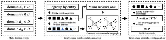
Figure 1.
The overall architecture of CDSTAEP: In CDSTAEP, we first divide the complex network data from different domains D, using the target host as the anchor point to separate the behavior sequence, form a correlation sequence of local events through behavior, and construct an event association graph based on the entity local event sequence. The blue square shows the intermediate sampling process of building a cross-domain event association graph, see Section 4.1.2 for details. Particularly, we feed the event correlation sequence and the constructed event association graph into the mixed-curvature GNN, and perform representation learning on the graph in the Riemannian space M, and the intermediate result of this step is output as a sequence of entity event vectors. At the same time, the entity event vector sequence is sent to the attention-based LSTM to obtain the relationship weight between events, and the final abnormal event prediction probability distribution is obtained through multi-layer perceptron (MLP). The final abnormal event prediction probability and accuracy comparison is shown in Algorithm 1.
4.1. Analysis and Representation of Entity-Level Cross-Domain Event Correlation
In the cross-domain network, an entity-level-based event correlation sequence and a local event correlation graph are first constructed, which is a prerequisite for a mixed-curvature representation of inter-event relations in Riemannian space. The correlation analysis in this paper is based on the horizontal cross-domain network environment and spatiotemporal association analysis of longitudinal time series. Details are as follows:
4.1.1. Demarcate Event Sequences with Entities as Anchors
In the cross-domain network , the edge in the graph is generated according to the interaction log between entity (i.e., user). In other words, one event may be generated by different entities, and one entity may generate multiple events. All the events generated by users at time t is , where is the number of entities in the dataset, and is the feature dimension of the event. Here, the event is represented by a tuple with a time dimension to facilitate the representation of cross-domain events in a certain time window.
The method of dividing the event sequence with the entity as the anchor point can refer to four dimensions, domain , entity , event and time (the event occurs). Each event corresponds to a timestamp , where the timestamp can be network time or a sequence number. If the event is generated by the same entity, the timestamp in the local process is . If the event is generated by different entities (i.e., interactive events), the timestamp of the event increased by one. Based on the data set, the event sequence generation method as shown in Figure 2.
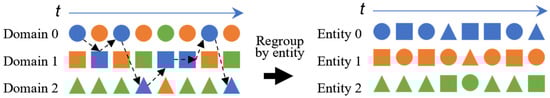
Figure 2.
Approach to generate event sequences: domains are used to distinguish different hosts, colors are used to distinguish different entities (i.e., users), and shapes are used to distinguish different events. The left side of the figure represents the time-ordered event sequence of the same event generated by different entities in the same domain (i.e., hosts). After data reorganization, the right side of the figure represents the time series of different events generated by the same entity, sorted by time, that is, the entity-level cross-domain event sequence.
The events generated by each entity are reorganized in chronological order to obtain entity-level cross-domain event sequences, as shown in the sequence of events for Entity 0 in Figure 2. For entity , the final sequence of events as follows:
where each 2-tuple is an event that occurs in domain at time . This is the data basis for the subsequent construction of event correlation diagrams.
4.1.2. Construction of Cross-Domain Event Association Graph Based on Entity Local Event Sequence
Based on the event sequence generated with entity as the target, we construct a local event sequence sliding window for each entity’s event sequence, and finally generate an overall cross-domain event association graph by traversing the event sequence, where is the comprehensive representation of the event, is the domain where the event occurs, is different events, and is the edge of the event association graph. As shown in Figure 3, since the size of the sliding window directly determines the complexity of the generated graph, the size of the sampling window should be set according to the computing power of the experimental environment.
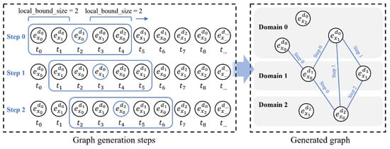
Figure 3.
The method of building a cross-domain event association graph: the left side of the figure is the sampling step, and here are three steps, namely Step 0, Step 1, and Step 2, and the sampling window local_bound_size = 2. The right side of the figure is the event association graph obtained after sampling, which contains both domain information and event category information.
For the convenience of plot representation, we set local_bound_size = 2 in the plot generation example. The size of bound_size determines the order in which the graph is generated and the relationship strength between the current node and the neighbor nodes. In experiments, to capture stronger relationship strength between nodes, we set bound_size = 10. Finally, the resulting graph is fully connected.
4.2. Graph Representation Learning in Mixed-Curvature Spaces
In large-scale data sets, the significance of association analysis is discovering hidden and valuable associations. The expert knowledge usually cannot effectively find these hidden relationships. In this paper, we use the graph engine to mine the relationship between data. In the mixed-curvature space, as shown in Table 3, the local correlation events in the generated graph are mostly tree structures, which are suitable for learning and representation in hyperbolic spaces; the global correlation events in the generated graphs are mostly ring structures, which are ideal for spherical space for learning representation; other associated events with low dimensions are ideal for learning representation using Euclidean space. The mixed-curvature space is constructed by the Cartesian product of multiple Riemannian spaces and combined with GNN to obtain the output representation of the mixed-curvature space [11,16]. Details are as follows:
4.2.1. Metric and Map Representations in Curvature Spaces
Theoretical foundations for graph representation learning in mixed-curvature spaces include:
(1) Euclidean Space
Euclidean space has curvature , and the space is uniform and flat everywhere, which is the result of the extension of geometric space measurement in linear space. It has space vector isotropy and translation invariance and is suitable for modeling grid data such as mesh data. Euclidean distance means the real distance between two points in n-dimensional space. In Riemann space, it is the geodesic length. The induced distance is as follows:
The exponential map of the Euclidean manifold is as follows:
where is the tangent space vector and is the point in manifold space .
The logarithmic map of the Euclidean manifold is as follows:
where is the point in manifold space .
(2) Hyperbolic Space
The curvature of the hyperbolic space . Since hyperbolic space has exponential volume capacity, the distance metric of hyperbolic space is equivalent to power-law distribution, and the tree structure can be embedded losslessly, it is very suitable for modeling ultra-large-scale hierarchical data and scale-free networks [11,15,35]. The existing Euclidean space models can be transformed into representation models in hyperbolic space through basic operators. The essence of hyperbolic space is a Riemannian manifold, which has the characteristics of local Euclidean geometry and can be expressed by various models, the most common of which is the Poincaré disc model. In the Riemannian space, the Poincaré model can be defined by the Riemannian manifold [25], and the Riemannian metric is as follows:
where is the Euclidean metric tensor and is the identity matrix. The hyperbolic metric tensor and the Euclidean metric tensor are conformal when the Poincaré sphere model represents the hyperbolic space embedding.
The norm-induced distance in the hyperbolic space is as follows:
For each tangent space , if , there is a specific one-to-one exponential mapping to map the space vector to the manifold . The exponential mapping function is as follows:
where the curvature , means the addition of space vectors, and any point , , is the Euclidean norm.
Logarithmic mapping is the inverse operation of exponential mapping, which can map points in manifold space to tangent space, realize data dimensionality reduction, and simplify calculations. That is, at point , , map the vector to tangent space . The logarithmic mapping function is as follows:
where k is the curvature in the Riemann space, any point , .
(3) Spherical Space
As in hyperbolic geometry, the embedding representation of hyperbolic spaces can be solved by the Poincaré model, as the solutions in spherical geometry [11]. The curvature of the spherical space , if , it is stretched into a spherical space with an infinite radius. Since the distance metric is equivalent to the angle metric and has rotation invariance, it is suitable for modeling ring data. The projected sphere model can well solve the representation problem of spherical space, the exponential and logarithmic mapping functions are as follows:
where is the standard Euclidean inner product, is the curvature in the Riemann space, any point , .
The spherical distance of is expressed as follows:
(4) Distance Representation in Mixed-Curvature Spaces
As shown in Formula (3), in the mixed-curvature space , for the node vector , its distance in the product space is defined as [9]. In other words, as shown in Formula (1), the distance can be expressed as the square distance between two points or as the Euclidean norm between two points. In addition, a simple distance representation method is introduced in some practical applications, and the geodesic method in the manifold structure is not used. For example, the distance is represented with the first-order norm , , where the minimum distance is . These distances provide simple and interpretable embedding spaces for mixed-curvature graphs.
4.2.2. Graph Representation Learning Based on Mixed-Curvature Spaces
To facilitate the representation learning of mixed-curvature graphs, we introduce the Cartesian product of multiple Riemannian component spaces to construct a mixed-curvature representation space . Then, we introduce a mixed-curvature GNN [16] with a hierarchical attention mechanism to complete the learned embedding of graphs with different curvatures in the mixed-curvature space . Particularly, GNN is divided into single-component space learning and cross-component space learning. Single-component space learning is used to learn the event correlation graph structure in fixed-curvature space. Cross-component space learning is used to fuse node representations in multi-curvature space, and it realizes the representation of event association graphs with multiple curvatures on mixed-curvature spaces.
(1) Fundamental Model
Stereographic projection models are used to fuse constant curvature spaces such as spheres, hyperboloids, and Euclidean manifolds [11]. For ease of calculation, we use κ-stereographic model to combine hyperbolic and spherical space. κ-stereographic model is a smooth manifold generated by the Riemannian metric , where the tensor is a point in the space, is the curvature of the manifold space, and the metric tensor is the conformal factor, expressed as follows:
Metric tensors are conformal, meaning all angles between tangent vectors in Riemann space remain constant. Computations in manifold structures usually ignore the difference between vectors caused by this angle.
is a three-dimensional spherical model, which is suitable for hyperbolic space when the curvature , and ideal for spherical space when the curvature . The operator, metric calculation, logarithmic mapping function, exponential mapping function in Euclidean space, and κ-stereographic model are shown in Formulas (7)–(16) and Table 4.
Table 4.
Basic operation formulas in Riemann space.
The key to representation learning is to obtain the representation of event relations in Euclidean space, hyperbolic space, and spherical space, respectively, and then fuse the node representation in mixed-curvature space to achieve the representation of complex relations between events.
(2) Single-Component Space Learning
In GNN, single-component space learning is used to learn the event association graph structure in the constant curvature space. In this layer, for a constant curvature space, we introduce Attention to learn to assign weights and aggregate the representations of all adjacent nodes . Since each neighbor node of has a different importance to , we introduce edge support to learn the importance of neighbor nodes. Specifically, we first use the logarithmic function to map the current node xi to the tangent space to use mature calculation methods in Euclidean space and use to model the importance of neighbor nodes. For an n-dimensional matrix , is the embedding dimension, and the edge support is calculated as follows:
where , is the Euclidean shared weight matrix, is the logistic sigmoid function , and denote the logarithmic map at the origin 0 in the κ-stereographic model. Then, normalize the calculation of the support:
where is the normalized edge support, is the index of the neighbor node of node in the graph, . Then, we use the self-loop in the attention-based GNN to keep the previous step information, that is, , is the identity matrix, and denote the exponential map at the origin 0 in the κ-stereographic model.
Next, the combination of support and representation is carried out. For the GNN, the expression of the relationship between nodes is to combine the embedding vectors of each node. This paper uses the combination of node support and node representation. In Euclidean space, the fusion of embedding vectors is given by the left multiplication [11,16] of the adjacency matrix of the embedding matrix with the embedding matrix, resulting in the matrix product . That is, the new representation of node is obtained by calculating the linear combination of all neighbor node embeddings of node , where the linear combination is weighted by the i-th row of the adjacency matrix . Particularly, matrix left multiplication is the basic operation on the value range of embedded vector ; that is, the result of matrix left multiplication is to obtain the change of the value of embedded vector , which is the latest result of vector fusion we expect to obtain. The right multiplication of the matrix is to change the base of the domain of the definition, so the result of the right multiplication is not what we expected.
We fuse the support of nodes with node representation through left matrix multiplication, and finally obtain node aggregate representation, including the support of all neighbor nodes. The calculation definition of the combination of support and representation is as follows:
where is the support adjacency matrix of embedded vector matrix , means κ-left-matrix-multiplication, , Euclidean midpoint function is defined as follows:
where has been defined in Formula (17).
In GNN, for a component space with any curvature , if the current layer is , then the input of layer is , and the output can be summarized as the following general expression:
where .
(3) Across-Component Spaces Learning
In GNN, cross-component space learning is used to fuse node representations from multiple different curvature spaces. First, in order to facilitate the subsequent calculation of GNN, we encode multi-curvature spaces in tangent space, calculate the mean value of node features in multi-curvature spaces through mean pooling, and perform forward propagation in the GNN model. The calculation formula for mean pooling is as follows:
where , is the Euclidean shared weight matrix, and
denotes the logarithmic map at the origin 0 in the κ-stereographic model.
Next, we calculate the support between nodes in different curvature spaces by :
where is the sigmoid. Next, we calculate the normalized support between nodes through the softmax function:
Finally, we connect the node representations from the multi-curvature space to obtain the fused weighted representation of the relationship nodes in the multi-curvature Riemannian space:
where means vector concatenation and means multiplication of space vectors.
The final output is the fused vector sequence in the Riemannian space, where means the Riemannian space.
(4) Self-Supervised Learning
The purpose of self-supervised learning is to learn rich correlations in samples by continuously optimizing the encoder function and obtain the event representation vector in the event associate graph by optimizing the objective function.
The effective comparison between positive and negative samples can enable the encoder to learn a richer feature representation, which is the basis of self-supervised learning. In self-supervised learning, views are generated by standard augmentations, such as cropping, rotation, etc., and defining views in Riemannian space is challenging. Two enhancement methods are generally considered on the graph: (1) feature space enhancement of the initial node, such as masking enhancement of sampling features or adding Gaussian noise; (2) generation of congruent graphs, such as generating congruence through diffusion matrix or the shortest distance picture. Research [45] shows that masking enhancement or adding noise in both spaces degrades the overall performance. Therefore, we transform the adjacency matrix into a diffusion matrix and treat these two matrices as two congruent graphs of the same graph structure, and then conduct sub-sampling. Since the adjacency matrix and the diffusion matrix, respectively, provide a local view and a global view of the graph structure, they can maximize the consistency of representing vectors from two different spaces, so that the self-supervised learning model can learn rich local information and global information through the encoder at the same time.
Contrastive learning is a particular case of self-supervised learning. The goal is to learn an encoder, the objective function [46], and compare the data with positive and negative samples in the feature space to learn the characteristics of the samples. For given data x, the similarity between positive and negative samples should satisfy the following:
where
is a node in the Riemann space, is a positive sample similar to , is a negative sample dissimilar to , and is usually the Euclidean distance or cosine similarity.
Comparing positive and negative samples in Riemannian space includes two methods: comparing positive and negative samples in the same curvature space and comparing positive and negative samples between different curvature spaces. We lift the samples in Riemannian space to a common tangent space and score the consistency of positive and negative samples from different curvature spaces to obtain richer feature representations [16]. The formula for calculating the similarity between positive and negative samples is as follows:
where is the node data, the logarithmic map is used to construct the common tangent space, and is the space curvature.
To optimize the encoder, it is necessary to construct a softmax classifier to classify positive and negative samples, and we introduce the Info NCELoss function [47] to optimize the encoder . The loss function formula in a single curvature space is as follows:
We evaluate the consistency between samples by the cosine similarity , where and are the encoding functions of positive and negative samples, respectively, and is the number of samples in a batch, that is, the number of all sampled nodes in the mixed-curvature space. For a given positive sample pair, the remaining samples are all negative samples. It can be seen from Equation (29) that the numerator only calculates the distance of the positive sample pair, and the negative sample only exists in the denominator. When the distance between the positive sample pair is smaller and the distance between the negative sample pair is larger, the loss is more minor.
The overall loss in a multi-curvature space is the sum of multiple single-curvature space losses, the formula is as follows:
Finally, after gradually optimizing through the above steps, a unified weighted representation of the event representation vector in the event association graph in the mixed-curvature space is obtained. The final output is a vector sequence, as shown in Formula (26).
4.3. Abnormal Behavior Prediction
This section aims to obtain weighted representations of event vectors via LSTM-ATT, including association fusion over time series. Ultimately, we use MLP to predict the probability that anomalous events may occur in subsequent periods. When the input feature vector sequence is too long, the traditional LSTM model has problems such as slow parameter update and gradient disappearance, which will increase the time complexity of model training and reduce the accuracy of the results. We introduce the Attention mechanism to solve the above problems by retaining intermediate results and calculating the support between related events in a targeted manner.
First, we convert the output of events in the mixed-curvature space to Euclidean space output to facilitate the computation of existing deep learning models. For multi-curvature spaces, the center point is , given the representation of an event in multiple curvature spaces, the Euclidean space output is , that is, the final conversion result is the combination of mixed-curvature space conversion vector with Euclidean space vector.
LSTM-ATT. Given a cross-domain event sequence of an entity in the time range to , where means different domains, is the event vector sequence obtained after characterization and input into the Attention-based LSTM model. As shown in Figure 4, for the convenience of expression, we denote the vector sequence value of as .
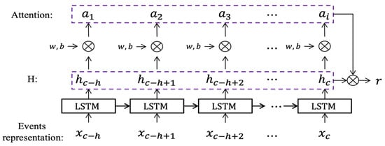
Figure 4.
Attention-based LSTM Model (LSTM-ATT): This model aims to calculate the weighted representation of the event vector. is the input event sequence, and are the weight vector and bias vector of the softmax layer, respectively, is the attention weight of each event.
For the sequence , the output of the LSTM cell is , respectively, and the attention calculation formula of each LSTM cell output is as follows:
where and are the weight vector and bias vector of the softmax layer.
The final output of Attention-based LSTM is the weighted representation of the associated event vector, as shown in Figure 4. The resulting formula is as follows:
We input the weighted event vector r into the MLP to obtain the final predicted probability of abnormal event occurrence. Since the MLP with one hidden layer can approximate the complex network system with arbitrary precision, this model introduces the MLP with one hidden layer. The output of the MLP hidden layer is as follows:
where and are the weight vectors between the hidden layer and the input layer and the bias vector of the hidden layer node, respectively, . The output of the MLP is as follows:
where is the weight vector between the hidden layer and the output layer, and is the bias vector of the output layer nodes. The activation function is defined as follows:
LOSS. This process will get a loss , which adopts cross entropy loss, which is as follows:
where is the output of the MLP model, and is the actual label of whether the output result is an abnormal event. If the predicted value approaches 1, which means that the probability of the event being anomaly increases, then the value of the loss function should approach 0. Conversely, if the predicted value y approaches 0, the value of the loss function should be very larger.
The overall loss function of CDSTAEP is:
where is the loss of graph representation learning in Formula (30). Through the optimization of the overall objective function, the ideal result of CDSTAEP is obtained.
4.4. Method Overview
The pseudo code of the algorithm in this paper is shown in Algorithm 1:
| Algorithm 1: CDSTAEP |
| Input: : the set of cross-domain event sequences; : the set of cross-domain event sequence tags. Output: : the set of vector representations of cross-domain events; : parameters for abnormal behavior prediction. 1: For 2: Generate sequence of events with Formula (6) 3: For 4: Generate cross-domain event association graph with the method in Figure 3 5: Initialize the event representation vector set 6: while not converging do 7: For each node in Riemannian space 8: For mixed-curvature space do//Update // 9: Single-Component Space Learning with Formula (29) 10: Across-Component Spaces Learning with Formula (30) 11: Calculate with Formulas (37) and (38)//Update neural network parameters &// 12: Until meet the condition for abnormal behavior prediction training |
5. Experiments and Evaluation
This section mainly evaluates the performance of CDSTAEP in predicting security events. Particularly, as a research result of a national key R&D project, this paper selects the real datasets collected by the project team in the live network to evaluate the performance of the proposed model. The purpose is to predict network behaviors such as illegal access and fraud in the live network. Furthermore, we compare the performance of CDSTAEP with other baseline models on real datasets.
5.1. Data Set
We selected the data set collected by a national key research and development project in the live network environment as the training set, and part of it as the test set. The continuous collection period was 30 days. The data set includes behavioral events such as network traffic, host process, and HTTP request. The event contains 21 fields, such as timestamp, host ID, event ID, the request method, process status, and the name of the user who initiated the event, involving 323,263 events. The primary characteristic data contained in the data set are shown in Table 5.
Table 5.
Examples of events data collected by a national key R&D plan.
Data Preprocessing. Since the intrusion behavior in the live network is less than the expected behavior and the sparsity is high, the method in Figure 5 is used to resample the intrusion behavior and normal behavior to generate a labeled normal and abnormal event sequence. In the end, we screened out 1505 normal host nodes from the data set, including five host nodes with sparse behavior and 301 abnormal host nodes.
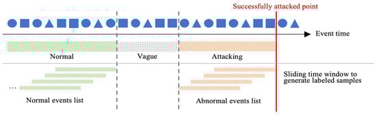
Figure 5.
Schematic representation of the data resampling method: The interval between normal events and abnormal events is (Vague) 10 min. The abnormal events (Attacking) time length is 20 min. The resampling window length is 10 min, and the sliding step is 1 min.
According to the resampled data, the event association graph generated by the experiment is shown in Figure 6. The actual local_bound_size = 10 in experiments; the larger the point in the graph, the larger the degree of the point.
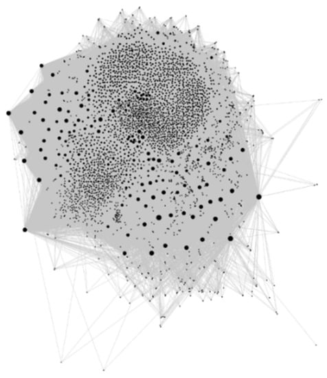
Figure 6.
Generated event association graph: The dots in the graph are visual representations of events in the association graph, and the larger the dots, the more events they are associated with. The event node information in the graph includes the event itself, domain, and time information, and the edges are the relationships between events.
5.2. Experimental Results
The experiment includes two aspects. First, analyze the influence of different curvature spaces on the prediction of abnormal events, and then analyze the prediction effect of CDSTAEP and the baseline model. We use the AUC score to evaluate the prediction performance of the proposed method.
5.2.1. Evaluation Criteria
This section defines the measurement of the evaluation classification model, that is, the accuracy of event prediction. Two evaluation criteria are adopted: area under roc curve (AUC), ACCURACY (ACC).
(1) ACC
ACC is the ratio of correctly predicted events to the total number of actual events in the test data set, which reflects the ability of the classification model to predict abnormal events. Acc needs to convert the prediction result probability of the classification model into a category before calculating the prediction accuracy, which is defined as follows:
where, is the predicted event, is the actual event, and is the total number of events in the test set. is used to judge whether is equal to or not. If they are the same, , otherwise . In fact, is a probability result, subject to the threshold of the classification model.
(2) AUC
The AUC randomly selects a sample from the positive sample and the negative sample, respectively. Then, it sets the probability that the positive sample is predicted to be 1 by the classifier as , and the probability that the negative sample is predicted to be 1 as , then ; that is, AUC means the sorting ability of the classifier to the samples, and is not limited by the threshold d. The result is used to measure the performance of the classification model.
Therefore, we adopt AUC as a criterion to evaluate the performance of classifier models. AUC is a probability, and the larger the value, the better the effect of the classifier (model). When , the effect of the classifier is a random selection, and the model has no predictive value; when , the prediction effect of the model is worse than that of random sampling; when , the classifier model has a better prediction effect when an appropriate threshold is set; when , the prediction result is grand truth, in specific application scenarios, and it is difficult for this kind of classifier to exist. The calculation formula of AUC is as follows:
where is the sorting of positive samples according to , M is the number of positive samples, is the number of negative samples, is all positive and negative sample pairs, M(1 + M)/2 is the sorted sum of the probability of repeated (positive, positive) samples.
5.2.2. Effect of Different Representation Spaces on Prediction of Abnormal Events
This experiment aims to compare and analyze the impact of different curvature spaces on anomaly prediction. To evaluate the proposed model’s ability to predict abnormal events better, we separate the representation learning part into single curvature space and mixed-curvature space.
CDSTAEP-H: Representation of event association graphs using hyperbolic spaces only.
CDSTAEP-S: Representation of event association graphs using only spherical spaces.
CDSTAEP-E: Representation of event association graphs using only Euclidean spaces.
CDSTAEP: Representation of event association graphs using mixed-curvature spaces.
After resampling the original data, we set the ratios of the training set to 0.2, 0.4, 0.6, and 0.8, respectively, and the rest as the test set. We recorded the results under different ratios of the training set. As shown in Figure 7 and Table 6, based on the same data set, the CDSTAEP-H, CDSTAEP-S, CDSTAEP-E, and CDSTAEP models all achieved good robustness in predicting abnormal events. The AUC score is better as the proportion of the training set increases, reflecting the fact that Riemannian spaces with different curvatures can effectively represent complex network data.
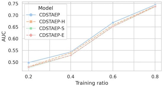
Figure 7.
Comparison of the effects of different representation spaces on event prediction: the horizontal axis is the ratio of the training set, and the vertical axis is the AUC score.
Table 6.
AUC for prediction by different representation spaces on the dataset.
Specifically, the data representation space of the CDSTAEP model is a mixed-curvature space. The result after classification by the abnormal behavior prediction model is better than the other models mentioned above. When the training ratio is 0.2, the difference in event prediction effect is the largest. The prediction effect of the CDSTAEP model is 0.4981, which is 1.80%, 2.19%, and 1.90% higher than that of CDSTAEP-H, CDSTAEP-S, and CDSTAEP-E, respectively. When the training ratio is 0.8, the AUC score of the CDSTAEP model is 0.7440, and the prediction effect is the best, which is 0.51%, 0.83%, and 0.67% higher than the prediction effect of CDSTAEP-H, CDSTAEP-S, and CDSTAEP-E respectively. There is less variance in the model’s predictive performance. The above experimental results show that the event association graph represented by the mixed-curvature space can retain more relationship features between events. The prediction effect is better than that represented by a single curvature space and has the strongest correlation with the prediction of abnormal events.
This experiment demonstrates that mixed-curvature spaces are suitable for representing complex network data and can capture rich event relationships. The comprehensive prediction effect of the CDSTAEP model is better than the performance of single-curvature space representation, but the difference is small. The reason is the sparsity of abnormal events in the real data, which leads to the relatively uniform distribution of abnormal events in the tree structure, ring structure, and network structure. Spaces with different curvatures are suitable for representing various types of data. Specifically, refer to the last column of Table 3.
5.2.3. CDSTAEP Model and Baseline Model
This experiment aims to compare multiple forecasting methods and analyze the contribution of event relationships to the prediction of abnormal events. To better evaluate the proposed forecasting model CDSTAEP, we choose two mainstream forecasting models, LSTM-ATT and LSTM, as baseline methods for comparison testing, and compared the time efficiency.
LSTM: It is a popular RNN recurrent neural network model in deep learning. Since it can selectively memorize long-term correlations, it is suitable for prediction tasks with time-dimensional characteristics.
LSTM-ATT: It is an LSTM model with an attention mechanism in deep learning. Since it can capture the weights of critical parts of the data set, it can implement prediction tasks in the time dimension in a targeted manner.
AUC score. After resampling the original data using the sliding window, we set the ratios of the training set to 0.2, 0.4, 0.6, and 0.8, respectively, and the rest as the test set. The prediction model CDSTAEP we proposed and the baseline methods LSTM-ATT and LSTM can predict time series data. Here, we mainly discuss the impact of adding cross-domain event relations on event prediction. Figure 8 and Table 7 record the comparison of the prediction effects of the three models under different training ratios.
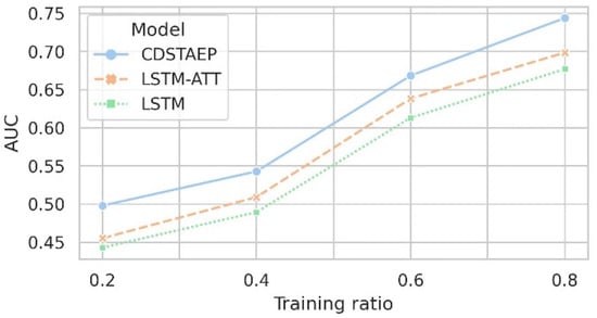
Figure 8.
Comparison of prediction effects of different models: the horizontal axis is the training ratio, and the vertical axis is the AUC score.
Table 7.
Time efficiency and AUC for different classifiers on the dataset.
As shown in Figure 8 and Table 7, under different proportions of training sets, the AUC score of the models CDSTAEP, LSTM, and LSTM-ATT for predicting abnormal events are relatively similar, and they all reflect good robustness. The prediction performance of LSTM-ATT is better than that of LSTM; in contrast, the prediction performance of the CDSTAEP model is the best. Due to the large sparsity of abnormal events in the data set, when the training ratio is low, the prediction results may be reversed. For example, when the training ratio is 20%, the AUC score of each model is less than 0.5. When the training ratio is 40%, the AUC score of LSTM is also less than 0.5. As the proportion of the training set increases, the comprehensive prediction effect shows an increasing trend. The AUC score of the CDSTAEP model increases from 0.4981 to 0.7440, and the best prediction effect is 4.53% and 6.69% higher than that of LSTM-ATT and LSTM, respectively. The difference is significant.
ACC score. Similarly, we compared ACC scores on the same data set. As shown in Figure 9 and Table 8, under the same training set proportion, the CDSTAEP model still obtains the highest scoring result compared with the LSTM-ATT and LSTM baseline models, similar to the AUC scoring results. Generally, in the existing network data set with no obvious abnormal features, the models using attention mechanism have achieved relatively good results. The accuracy of CDSTAEP model is 5.5% and 11.5% higher than LSTM-ATT and LSTM, respectively.
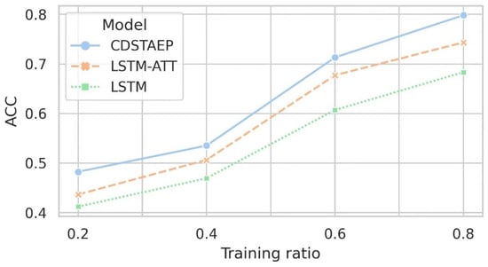
Figure 9.
Comparison of prediction effects of different models: the horizontal axis is the training ratio, and the vertical axis is the ACC score.
Table 8.
Time efficiency and ACC for different classifiers on the dataset.
Time efficiency. In the actual application scenarios, the detection and prediction of abnormal events, the time efficiency of the classifier is an important factor in evaluating the model. Based on the original data set, which contains 301 abnormal host nodes, the overall prediction time of the CDSTAEP model is compared with the baseline method, as shown in Table 7. Since the model training is offline and the training time is related to computing power, the time consumption in the abnormal reasoning stage is more important to evaluate the model. As can be seen from the comparison result, because the model CDSTAEP is more complicated, the time efficiency of the reasoning stage is not the best. Compared with the model classification effect, this is acceptable.
Overall, the prediction effect of the CDSTAEP model is better than that of LSTM-ATT and LSTM, and regardless of the training ratio, it can achieve better results and is more robust. The LSTM model only considers the time dependence between events but does not consider the intra-domain and cross-domain dependencies between events, resulting in a slightly poorer prediction effect. The LSTM-ATT model considers the attention of essential features based on LSTM but still does not consider the relationship between events. Therefore, the prediction effect is slightly better than LSTM and slightly worse than CDSTAEP. The above results show that the CDSTAEP model can stably improve the performance of the selected classifiers and prove the embedded representation of complex network events in the mixed-curvature space while introducing dependencies such as time, inter-domain (between hosts), and between events, which can effectively improve the accuracy of abnormal event prediction.
5.3. Discussion
Limitations of the CDSTAEP model. First, because the CDSTAEP model relies on the representation learning results of historical log when deployed online, it will face problems such as changes in the network structure and new events, resulting in repeated training of the model. Second, CDSTAEP incorporates spatial relationships between domains, entities, and events, as well as temporal relationships between events, but faces difficulties in effectively fusing behaviors, more complex attributes of events (e.g., threat level, threat type). Integrating more information can predict events in a more targeted manner and more effectively improve the possibility of predicting unknown abnormal events.
Future work. Future work will focus on how to represent dynamic, multi-dimensional, and complex attribute information in the Riemannian space, effectively integrate more dimensional attribute vectors, improve the prediction effect of abnormal network events, and provide more effective countermeasures for active network defense.
6. Conclusions
This paper proposes an abnormal event prediction model CDSTAEP, which is based on an event association graph and mixed-curvature space representation. Most of the existing network abnormal event prediction methods are based on time features or the spatiotemporal features associated with hosts, embedding events in Euclidean space, using the LSTM model and its improved model, hidden Markov model, etc., to predict future events. However, this approach, which relies on the relationship between event time and hosts, does not consider the correlation between events. To simultaneously capture, characterize, and fuse the time, inter-domain (between hosts), and inter-space dependencies of events, the prediction model proposed in this paper captures the relationship between cross-domain events in the Riemannian space.
First, we used a data set of a national key research and development plan, used the entity as the anchor, and referred to the three dimensions of the domain, time, and event to generate entity-level cross-domain event sequences, and then constructed a cross-domain event association graph. On this basis, we took advantage of the mixed-curvature space to better characterize complex network relationships and introduce event relationships into the final expression of event features. We use the mixed-curvature GNN to obtain the representation of the entity event vector sequence to capture the spatial relationship between events. At the same time, combined with the mixed-curvature vector representation of the events, LSTM-ATT was used to capture the temporal relationship characteristics of the events. Then, combined with the spatiotemporal vector representation of the events, self-supervised learning was used to obtain the fusion representation X of the spatiotemporal features of the events. Sending X into MLP, by optimizing the overall objective function, a better prediction effect was obtained. The experimental results show that the CDSTAEP model can obtain better event prediction results than LSTM, LSTM-ATT.
Author Contributions
Conceptualization, M.G.; methodology, M.G.; software, M.G. and R.W.; validation, M.G., H.Z. and R.W.; formal analysis, M.G., H.Z. and R.W.; investigation, M.G., H.Z., R.W. and Y.X.; resources, H.Z. and Y.X.; data curation, H.Z. and R.W.; writing—original draft preparation, M.G.; writing—review and editing, M.G., H.Z., R.W. and Y.X.; visualization, M.G. and R.W.; supervision, H.Z. and Y.X.; project administration, M.G. and Y.X.; funding acquisition, H.Z. and Y.X. All authors have read and agreed to the published version of the manuscript.
Funding
This work was supported by the National Key R&D Program of China under Grant 2020YFB1708600, 2018YFB0804500.
Institutional Review Board Statement
Not applicable.
Informed Consent Statement
Not applicable.
Data Availability Statement
For reasons related to the project, we do not provide the dataset for now.
Conflicts of Interest
The authors declare no conflict of interest.
References
- Liu, Y.; Zhang, J.; Sabari, A.; Liu, M.; Karir, M.; Baily, M. Predicting cyber security incidents using feature-based characterization of networklevel malicious activities. In Proceedings of the 2015 ACM International Workshop on International Workshop on Security and Privacy Analytics, San Antonio, TX, USA, 4 March 2015; pp. 3–9. [Google Scholar]
- Husak, M.; Komarkova, J.; Bou-Harb, E.; Celeda, P. Survey of attack projection, prediction, and forecasting in cyber security. IEEE Commun. Surv. Tuts. 2019, 21, 640–660. [Google Scholar] [CrossRef]
- Soska, K.; Christin, N. Automatically detecting vulnerable websites before they turn malicious. In Proceedings of the 23rd USENIX Security Symposium, San Diego, CA, USA, 20–22 August 2014; pp. 625–640. [Google Scholar]
- Xu, K.; Wang, F.; Gu, L. Network-aware behavior clustering of internet end hosts. In Proceedings of the 2011 Proceedings IEEE INFOCOM, Shanghai, China, 10–15 April 2011; pp. 2078–2086. [Google Scholar]
- Chen, Y.; Huang, Z.; Lai, Y. Spatiotemporal patterns and predictability of cyberattacks. PLoS ONE 2015, 10, e0124472. [Google Scholar] [CrossRef] [PubMed]
- Kipf, T.; Welling, M. Semi-supervised classification with graph convolution network. arXiv 2016, arXiv:1609.02907. [Google Scholar]
- Papadopoulos, F.; Kitsak, M.; Serrano, M.Á.; Boguñá, M. Popularity versus Similarity in Growing Networks. Nature 2013, 489, 537–540. [Google Scholar] [CrossRef]
- Shen, Y.; Mariconti, E.; Vervier, P.-A.; Stringhini, G. Tiresias: Predicting security events through deep learning. In Proceedings of the 2018 ACM SIGSAC Conference on Computer and Communications Security, Toronto, ON, Canada, 15–19 October 2018; pp. 592–605. [Google Scholar]
- Gu, A.; Sala, F.; Gunel, B.; Ré, C. Learning Mixed-Curvature Representations in Product Spaces. In Proceedings of the International Conference on Learning Representations 2018, Vancouver, BC, Canada, 30 April–3 May 2018. [Google Scholar]
- Defferrard, M.; Perraudin, N.; Kacprzak, T.; Sgier, R. Deepsphere: Towards an equivariant graph-based spherical cnn. In Proceedings of the ICLR Workshop on Representation Learning on Graphs and Manifolds, New Orleans, LA, USA, 6 May 2019. [Google Scholar]
- Bachmann, G.; Gary, B.; Octavian-Eugen, G. Constant Curvature Graph Convolutional Networks. arXiv 2019, arXiv:1911.05076. [Google Scholar]
- Fu, X.; Li, J.; Wu, J.; Sun, Q.; Ji, C.; Wang, S.; Tan, J.; Peng, H. ACE-HGNN: Adaptive Curvature Exploration Hyperbolic Graph Neural Network. In Proceedings of the 2021 IEEE International Conference on Data Mining (ICDM), Auckland, New Zealand, 7–10 December 2021; IEEE: New York, NY, USA, 2021; pp. 111–120. [Google Scholar]
- Liu, Q.; Nickel, M.; Kiela, D. Hyperbolic graph neural networks. Adv. Neural Inf. Process. Syst. 2019, 32, 8228–8239. [Google Scholar]
- Krioukov, D.; Papadopoulos, F.; Vahdat, A.; Boguná, M. On curvature and temperature of complex networks. Phys. Rev. E 2009, 80, 035101. [Google Scholar] [CrossRef]
- Krioukov, D.; Papadopoulos, F.; Kitsak, M.; Vahdat, A.; Boguná, M. Hyperbolic Geometry of Complex Networks. Phys. Rev. E 2010, 82, 036106. [Google Scholar] [CrossRef]
- Sun, L.; Zhang, Z.; Ye, J.; Peng, H.; Zhang, J.; Su, S.; Philip, S.Y. A Self-supervised Mixed-curvature Graph Neural Network. In Proceedings of the AAAI Conference on Artificial Intelligenc, Virtually, 22 February–1 March 2022. [Google Scholar]
- Cheng, Q.; Shen, Y.; Kong, D.; Wu, C. STEP: Spatial-Temporal Network Security Event Prediction. arXiv 2021, arXiv:2105.14932. [Google Scholar]
- Tan, L.; Pham, T.; Ho, H.K.; Kok, T.S. Event Prediction in Online Social Networks. J. Data Intell. 2021, 2, 64–94. [Google Scholar] [CrossRef]
- Xu, M.; Schweitzer, K.M.; Bateman, R.M.; Xu, S. Modeling and Predicting Cyber Hacking Breaches. IEEE Trans. Inf. Forensics Secur. 2018, 13, 2856–2871. [Google Scholar] [CrossRef]
- Condon, E.; He, A.; Cukier, M. Analysis of Computer Security Incident Data Using Time Series Models. In Proceedings of the 2008 19th International Symposium on Software Reliability Engineering (ISSRE), Seattle, WA, USA, 10–14 November 2008; IEEE: New York, NY, USA, 2008; pp. 77–86. [Google Scholar]
- Huang, C.; Deep, A.; Zhou, S.; Veeramani, D. A deep learning approach for predicting critical events using event logs. Qual. Reliab. Eng. Int. 2021, 37, 2214–2234. [Google Scholar] [CrossRef]
- Perry, I.; Li, L.; Sweet, C.; Su, S.-H.; Cheng, F.-Y.; Yang, S.J.; Okutan, A. Differentiating and Predicting Cyberattack Behaviors Using LSTM. In Proceedings of the 2018 IEEE Conference on Dependable and Secure Computing (DSC), Kaohsiung, China, 10–13 December 2018; pp. 1–8. [Google Scholar]
- Wang, Z.; Wu, Y.; Li, Q.; Jin, F.; Xiong, W. Link prediction based on hyperbolic mapping with community structure for complex networks. Phys. A Stat. Mech. Its Appl. 2016, 450, 609–623. [Google Scholar] [CrossRef]
- Ara, Z.; Hashemi, M. Traffic Flow Prediction using Long Short-Term Memory Network and Optimized Spatial Temporal Dependencies. In Proceedings of the 2021 IEEE International Conference on Big Data, Orlando, FL, USA, 15–18 December 2021; pp. 1550–1557. [Google Scholar]
- Ganea, O.; Bécigneul, G.; Hofmann, T. Hyperbolic neural networks. In Advances in Neural Information Processing Systems; The MIT Press: Cambridge, MA, USA, 2018; pp. 5345–5355. [Google Scholar]
- Rezaabad, A.L.; Kalantari, R.; Vishwanath, S.; Zhou, M.; Tamir, J. Hyperbolic Graph Embedding with Enhanced Semi-Implicit Variational Inference. In International Conference on Artificial Intelligence and Statistics; PMLR: New York, NY, USA, 2021. [Google Scholar]
- Gulcehre, C.; Denil, M.; Malinowski, M.; Razavi, A.; Pascanu, R.; Hermann, K.M.; Battaglia, P.; Bapst, V.; Raposo, D.; Santoro, A.; et al. Hyperbolic Attention Networks. arXiv 2018, arXiv:1805.09786. [Google Scholar]
- Chami, I.; Gu, A.; Chatziafratis, V.; Ré, C. From trees to continuous embeddings and back: Hyperbolic hierarchical clustering. Adv. Neural Inf. Process. Syst. 2020, 33, 15065–15076. [Google Scholar]
- Serrano, M.; Krioukov, D.; Boguñá, M. Self-similarity of complex networks and hidden metric spaces. Phys. Rev. Lett. 2008, 100, 078701. [Google Scholar] [CrossRef] [PubMed]
- Zhu, Y.; Zhou, D.; Xiao, J.; Jiang, X.; Chen, X.; Liu, Q. HyperText: Endowing FastText with Hyperbolic Geometry. arXiv 2020, 1166–1171. [Google Scholar] [CrossRef]
- Zhuang, C.; Qiang, M. Dual Graph Convolutional Networks for Graph-Based Semi-Supervised Classification. In Proceedings of the 2018 World Wide Web Conference, Lyon, France, 23–27 April 2018; pp. 499–508. [Google Scholar]
- Zhang, Y.; Wang, X.; Shi, C.; Liu, N.; Song, G. Lorentzian Graph Convolutional Networks. In Proceedings of the Web Conference 2021, Ljubljana, Slovenia, 19–23 April 2021; pp. 1249–1261. [Google Scholar]
- Chen, Y.; Yang, M.; Zhang, Y.; Zhao, M.; Meng, Z.; Hao, J.; King, I. Modeling Scale-free Graphs with Hyperbolic Geometry for Knowledge-aware Recommendation. In Proceedings of the Fifteenth ACM International Conference on Web Search and Data Mining, Tempe, AZ, USA, 21–25 February 2022; pp. 94–102. [Google Scholar]
- Tay, Y.; Tuan, L.A.; Hui, S.C. Hyperbolic Representation Learning for Fast and Efficient Neural Question Answering. In Proceedings of the Eleventh ACM International Conference on Web Search and Data Mining, Los Angeles, CA, USA, 5–9 February 2018; pp. 583–591. [Google Scholar]
- Nickel, M.; Kiela, D. Learning Continuous Hierarchies in the Lorentz Model of Hyperbolic Geometry. In International Conference on Machine Learning; PMLR: Birmingham, UK, 2018. [Google Scholar]
- Sun, L.; Zhang, Z.; Zhang, J.; Wang, F.; Peng, H.; Su, S.; Yu, P.S. Hyperbolic Variational Graph Neural Network for Modeling Dynamic Graphs. Proc. Conf. AAAI Artif. Intell. 2021, 35, 4375–4383. [Google Scholar] [CrossRef]
- Cruceru, C.; Becigneul, G.; Ganea, O.-E. Computationally Tractable Riemannian Manifolds for Graph Embeddings. Proc. Conf. AAAI Artif. Intell. 2021, 35, 7133–7141. [Google Scholar] [CrossRef]
- Wang, S.; Wei, X.; Nogueira dos Santos, C.N.; Wang, Z.; Nallapati, R.; Arnold, A.; Xiang, B.; Yu, P.S.; Cruz, I.F. Mixed-Curvature Multi-Relational Graph Neural Network for Knowledge Graph Completion. In Proceedings of the Web Conference 2021, Ljubljana, Slovenia, 19–23 April 2021. [Google Scholar]
- Park, H.; Jung, S.-O.D.; Lee, H.; In, H.P. Cyber Weather Forecasting: Forecasting Unknown Internet Worms Using Randomness Analysis. In Information Security and Privacy Research: 27th IFIP TC 11 Information Security and Privacy Conference, SEC 2012, Heraklion, Crete, Greece, 4–6 June 2012; Springer: Berlin/Heidelberg, Germany, 2012; pp. 376–387. [Google Scholar]
- Soldo, F.; Le, A.; Markopoulou, A. Markopoulou Blacklisting recommendation system: Using spatio-temporal patterns to predict future attacks. IEEE J. Sel. Areas Commun. 2011, 29, 1423–1437. [Google Scholar] [CrossRef]
- Zhan, Z.; Xu, M.; Xu, S. Predicting cyber attack rates with extreme values. IEEE Trans. Inf. Forensics Secur. 2015, 10, 1666–1677. [Google Scholar] [CrossRef]
- Xiong, B.; Zhu, S.; Potyka, N.; Pan, S.; Zhou, C.; Staab, S. Semi-Riemannian Graph Convolutional Networks. arXiv 2021, arXiv:2106.03134. [Google Scholar]
- Skopek, O.; Ganea, O.E.; Bécigneul, G. Mixed-curvature variational autoencoders. arXiv 2019, arXiv:1911.08411. [Google Scholar]
- Chang, S.; Han, W.; Tang, J.; Qi, G.J.; Aggarwal, C.C.; Huang, T.S. Heterogeneous Network Embedding via Deep Architectures. In Proceedings of the 21th ACM SIGKDD International Conference on Knowledge Discovery and Data Mining, Sydney, Australia, 10–13 August 2015; pp. 119–128. [Google Scholar]
- Hassani, K.; Khasahmadi, A.H. Contrastive multi-view representation learning on graphs. In International Conference on Machine Learning; PMLR: New York, NY, USA, 2020. [Google Scholar]
- Chen, T.; Kornblith, S.; Swersky, K.; Norouzi, M.; Hinton, G.E. Big self-supervised models are strong semi-supervised learners. Adv. Neural Inf. Process. Syst. 2020, 33, 22243–22255. [Google Scholar]
- Oord, A.V.; Li, Y.; Vinyals, O. Representation learning with contrastive predictive coding. arXiv 2018, arXiv:1807.03748. [Google Scholar]


Disclaimer/Publisher’s Note: The statements, opinions and data contained in all publications are solely those of the individual author(s) and contributor(s) and not of MDPI and/or the editor(s). MDPI and/or the editor(s) disclaim responsibility for any injury to people or property resulting from any ideas, methods, instructions or products referred to in the content. |
© 2023 by the authors. Licensee MDPI, Basel, Switzerland. This article is an open access article distributed under the terms and conditions of the Creative Commons Attribution (CC BY) license (https://creativecommons.org/licenses/by/4.0/).