Article

Combining the Transformer and Convolution for Effective Brain Tumor Classification Using MRI Images

1
Department of Electrical Engineering, College of Engineering, Qassim University, Unaizah 56452, Saudi Arabia
2
Department of Computer Science, Islamia College Peshawar, Peshawar 25120, Pakistan
3
Department of Information Technology, College of Computer, Qassim University, Buraydah 51452, Saudi Arabia
4
Department of Electrical Engineering, College of Engineering and Information Technology, Onaizah Colleges, Onaizah 56447, Saudi Arabia
*
Author to whom correspondence should be addressed.
Appl. Sci. 2023, 13(6), 3680; https://doi.org/10.3390/app13063680
Submission received: 14 December 2022 / Revised: 7 February 2023 / Accepted: 9 February 2023 / Published: 14 March 2023
(This article belongs to the Special Issue Future Internet of Things: Applications, Protocols and Challenges)

Abstract

:
In the world, brain tumor (BT) is considered the major cause of death related to cancer, which requires early and accurate detection for patient survival. In the early detection of BT, computer-aided diagnosis (CAD) plays a significant role, the medical experts receive a second opinion through CAD during image examination. Several researchers proposed different methods based on traditional machine learning (TML) and deep learning (DL). The TML requires hand-crafted features engineering, which is a time-consuming process to select an optimal features extractor and requires domain experts to have enough knowledge of optimal features selection. The DL methods outperform the TML due to the end-to-end automatic, high-level, and robust feature extraction mechanism. In BT classification, the deep learning methods have a great potential to capture local features by convolution operation, but the ability of global features extraction to keep Long-range dependencies is relatively weak. A self-attention mechanism in Vision Transformer (ViT) has the ability to model long-range dependencies which is very important for precise BT classification. Therefore, we employ a hybrid transformer-enhanced convolutional neural network (TECNN)-based model for BT classification, where the CNN is used for local feature extraction and the transformer employs an attention mechanism to extract global features. Experiments are performed on two public datasets that are BraTS 2018 and Figshare. The experimental results of our model using BraTS 2018 and Figshare datasets achieves an average accuracy of 96.75% and 99.10%, respectively. In the experiments, the proposed model outperforms several state-of-the-art methods using BraTS 2018 and Figshare datasets by achieving 3.06% and 1.06% accuracy, respectively.

1. Introduction

Brain tumors (BTs) are considered one of the leading types of cancer throughout the globe [1,2]. It is essential to detect and localize the BT in the initial stage to save human lives. There are two types of BT that are Benign and Cancerous (malignant) tumors. The benign BT is a low-grade tumor, where a patient has a high chance of survival. The malignant BT is a high-grade tumor, which can quickly spread to other regions of the body and it is difficult to treat [3,4]. Therefore, selecting a precise treatment strategy requires early detection of the correct type and grade of malignancy.
An efficient method to identify BT is to look at the patient’s Magnetic Resonance Imaging (MRI) scans of their brain [5]. MRI is one of the most common methods that is used to scan a brain under the influence of a very strong magnetic field. MRI uses radiofrequency signals to excite the target tissue so that a picture of its interior can be made. It is effective because it shows soft tissue well and does not expose the patient to any ionizing radiation. Hence, the MRI is commonly used for finding problems in the brain [6,7,8].
Due to significant variability and inherent MRI data properties, i.e., variability in tumor shapes, and sizes, analyzing the affected region, and finding uncertainty in the segmented areas, BT is a difficult task to perform. Tumor classification is the most significant problem in BT image analysis. Examples of applications include tumor volume estimation, tissue classification, blood cell delineation, tumor localization, atlas matching, surgical planning, and image registration. The morphological and precise tumor quantification is a critical task for observing oncologic therapy. Although substantial work has been carried out in this field, physicians are still dependent on manual tumor detection, which is time-consuming and tedious work. The emergence of new technologies, particularly ML and deep learning, has a significant influence in the healthcare sector. As a results, machines have been used as a second opinion for early disease detection [9,10]. Since it has given medical departments including medical imaging an essential support tool to interpret MRI images and support the radiologist’s choice, a variety of machine and deep learning algorithms are used for segmentation and classification.
There have been many Computer-Aided Diagnostic (CAD) systems used by radiologists in recent years that are based on ML [9]. To determine if a tumor is normal or pathological, the earliest models for tumor prediction relied on feature representations such as wavelet features and ML algorithms. The subsequent class of models use various sets, i.e., boundary, texture, and form of features simultaneously, which are high dimensional characteristics that are reduced to generate features maps. These feature maps are trained using an ensemble of classifiers including Artificial Neural Network (ANN), K-Nearest Neighbor (k-NN), and Support Vector Machine (SVM) [11]. Khalid et al. exploited intensity, neighborhood, and wavelet characteristics of brain MRI images as features. These features are merged and fed to random forest classifiers to forecast varying tumor levels [12]. In texture-based characteristics, an SVM classifier, and deep neural networks are used to classify BT [13].
Convolutional Neural Networks (CNN) quickly supplant traditional machine learning approaches in numerous application domains [14,15,16,17,18,19,20]. The CNN contains four basic layers such as a convolutional layer, a pooling layer, a fully connected layer, and an output layer. The convolutional layer is responsible for optimum feature extraction from the given input images by using different kinds of filters including edges, colors, shapes, etc. Afterward, the extracted features maps are subjected to a pooling layer for dimensionality reduction [21], there are three different types of pooling operation such as maximum pooling, minimum pooling, and average pooling. Furthermore, in the fully connected layer, each neuron of the previous layer is differently connected to the next layer neuron similar to mesh topology in the network [22]. Finally, the output layer is responsible for class prediction by assigning labels to each class. Figure 1 shows the overall structure of the CNN. Some CNN architecture for the categorization of tumor and normal MRI images was implemented in [23,24]. Furthermore, CNNs were employed to partition the damaged tissues of the brain from the non-tumor regions in [25], in addition to being used in tumor categorization. To better categorize BT, a capsule network architecture was developed in [26]. BT classification is an example of many medical image analysis tasks where pre-trained CNN networks have been used to improve classification accuracy in recent studies [27].
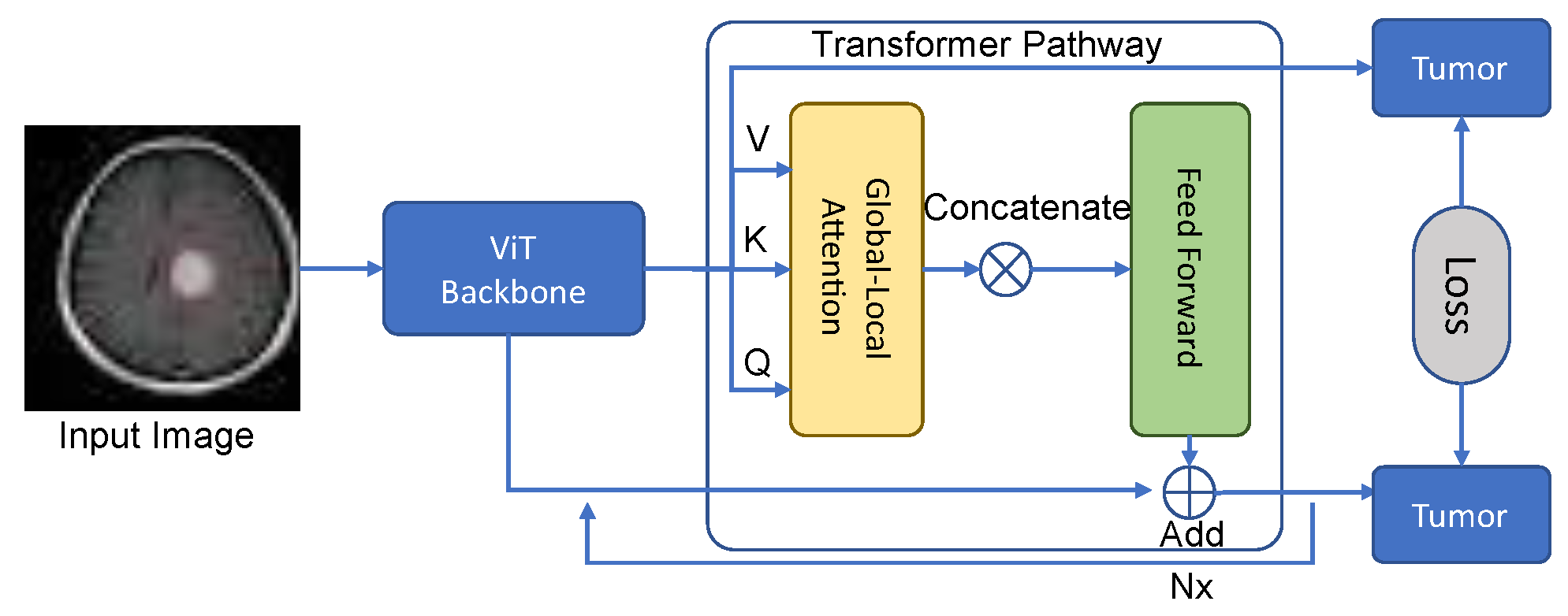
To assist radiologists in visualizing [6,23,25] and classifying tumor types [7], multi-grade BT categorization systems, or CAD, have been developed. Deep neural networks are used to classify various grades using high-level data taken from MRI scans, which may aid radiologists in making choices regarding early diagnosis and potential treatment modalities. This classification, offered by many researchers, provides information regarding the percentage of malignant tumors. The main issues with current methods for classifying BT are binary categorization, a paucity of data samples for various grades, and poor accuracy. With only two categories (benign and malignant) for BT classification, the methods used now make it exceedingly difficult for radiologists to proceed with additional testing or treatment. The lack of publicly available data is another main obstacle in the classification of BT. Additionally, the current methods have not yet demonstrated satisfactory accuracy. For these reasons, we suggest a “transformer-enhanced convolutional Neural network (TECNN)” for tumor classification. The Transformer is first proposed by Dosovitskiy et al. [28]. for image analysis, which utilized a standard Transformer structure directly to the images. In the Transformer structure, an image is divided into various image patches, afterword these patches are subjected to a Transformer encoder as shown in Figure 2. The Transformer treats these patches as tokens similar to Naturel Language Processing (NLP). After the encoding layer, the classification layer is used for accurate categorization. In the proposed TECNN we use two primary parts, (1) features extraction using CNN, and (2) a transformer, as shown in Figure 3. We use features extraction to extract the local features using CNN that focuses on pixel-wise information by using various convolutional and pooling layers. The Transformer focuses on the patch-wise information instead of focusing on pixels. Initially, the convolution operation is applied to a given image before feeding them to our proposed model. The feature extractor and transformer pipeline are each individually fed with the processed image at this point. The Transformer patch embeddings (PE) and sets of CNN’s feature maps have different dimensions, and as a result, there is a clear semantic gap between them. We use the feature fusion module (FFM) and intelligent merge module (IMM), as proposed by Chen et al. [29] so that the CNN and transformer techniques could be used to convert between feature maps and patches while maintaining their benefits. Both the feature extraction using CNN and transformer provide inputs to the FFM and IMM. The CNN’s feature maps are transformed into transformer space in the FFM and fused with transformer patches. Global pooling (GP) is used to choose an informative channel of the given input feature maps rather than performing a straight conversion. Channels with more class-specific functionality are emphasized in this section. The transition from feature maps to patches is thus considerably more seamless. CNN’s local information guidance can be spread to the transformer patches. The output of the FFM is then fused using the class token as shown in Figure 3. The input of Transformer is firstly converted to a feature map in the IMM, and then it undergoes trough average pooling (AG). The class-sensitive channels of the pooled features are then highlighted using a channel-wise attention technique [26]. Next, the input of the transformer is adaptively fused with CNN feature maps to improve the long-rang dependency. Local information and global features are both retained in the aggregated features. This hybrid structure enables our model to efficiently perform BT classification. The major contributions of our work are highlighted as follows:
  • We propose a hybrid model that extracts local as well as retains global information simultaneously for an effective BT classification.
  • In the proposed work the FFM and IMM models are employed, the FFM module is responsible for converting the CNN feature maps to PE, while the IMM is responsible for fusion between the feature maps, PE an adaptive and intelligent process.
  • Our model has been evaluated on two publicly available datasets and the experimental results of our model for BT classification outperforms state-of-the-art methods.
Figure 2. Shows the Vision Transformer architecture proposed by Dosovitskiy et al. [28].
Applsci 13 03680 g002
Figure 3. Our proposed framework for brain tumor classification.
Applsci 13 03680 g003
The remaining paper is organized in the following manners. Section 2 describes the related research work in the field of BT classification, and Section 3, provides information about the proposed architecture. Section 4 shows experimental results and Finally, Section 5 concludes this work.

2. Literature Review

In recent years, researchers have previously examined various medical image diagnosis techniques based on ML and DL methods [30,31,32,33,34]. The discipline of medical image analysis, particularly the field of disease identification, has benefited immensely from the introduction of new technologies involving deep learning and artificial intelligence. There have been numerous studies on CNN-based BT multiclassification and tumor detection. There are several ways to approach the research in the literature. For instance, some researchers have used CNN models that they have independently created to do BT classification, while other researchers have achieved the same goal by using transfer learning strategies. Talo et al. [35], recommended using the pre-trained pipeline named the ResNet-34 CNN model when utilizing MRI data to identify BTs. In addition, their proposed model obtained optimal performance in terms of accuracy using a publicly available dataset. Furthermore, their proposed model is capable of accurately classifying BT such as meningioma, glioma, and pituitary tumors. Another approach presented by Rehman et al. [36], used different pre-trained architectures (namely AlexNet, GoogleNet, and VGG16) with some fine-tuning strategies to classify the BT into benign or malignant classes. They used a publicly available MRI dataset of 233 patients and achieved accuracy of 98.69%. A later approach was introduced by Mehrotra et al. [37], applied a transfer learning technique based on Deep Learning (DL) which categorizes the BTs into benign and malignant. Their experimental work is focused on the pre-trained CNN-based architectures known as ResNet101, ResNet50, GoogleNet, AlexNet, and SqueezeNet. The AlexNet gives a comparatively promising performance as compared to other models. Another approach devised by Khan et al. [38], utilized MRIs dataset with data augmentation technique to enhance the performance of the proposed method for accurate classification of BT. They employed an edge detection method on region of interest (ROI) that is selected before extracting the data from an MRI image using a typical CNN model. In addition, their proposed model obtained high performance in terms of evaluation matrices such as precision. BT classification using a CNN-based Computer-Assisted Diagnosis (CAD) method was developed by Ayadi et al. [39]. Three different datasets were employed in trials with the 18-weighted layered CNN model, and obtained 90.35% of tumor rating accuracy and 94.74% classification accuracy. In order to predict tumor grade without the aid of expert annotations of regions of interest, Pereira et al. [40] employed CNN in 2018. They compared two methods of prediction: one used data from the entire brain and the other one used data from an artificially identified tumor location. They obtained 89.5% accuracy with the grade prediction from the complete brain image and also obtained 92.98% accuracy with the grade prediction from the tumor ROI. The two models are completely connected and convolution neural networks are proposed by Paul et al. [41] who also conduct classification using a dataset with three classes divided into three separate planes. The authors simply assessed the model by just selecting the axial plane for performance accuracy in order to prevent any confusion for the model between the three different planes. Their experimental results showed that the CNN is optimally better, with a 91.43% accuracy rate. Jude Hemanth et al. [42], implemented a CNN-based model for diagnosing brain disorders. They achieved that by resolving the convergence time period constraints of ANNs when employing MRI. To do this, they implemented two modified models of the Counter Propagation Neural model (CPN) and the Kohonen Neural Network (KNN), referred to as MCPN and MKNN, respectively. Their primary goal was to create the ANN models in such a way that they can solve the convergence rate. They were successful in doing so, and after altering the accuracy rate, they achieved 95% accuracy for MKNN and 98% accuracy for MCPN.
Abiwinanda et al. [43] suggestion was to investigate the basic CNN model without making any modifications, merely working on CNN and adjusting the number of its various layers. They created seven alternative CNN designs in this way, each with a different number of layers, and concluded that the second architecture, achieved a training accuracy of 98.51% that consisted of two layers of convolution, activation, and max pooling, is the best of all of them. Zhou et al. [44], proposed a model that employed direct holistic 3D reconstruction of an image. The DenseNet was then used to extract features from the two-dimensional slices after first converting the three-dimensional holistic image into two-dimensional slices. A recurrent neural network model was created and tested to categorize the images. Two separate datasets, one private and the other public were used for testing. The DenseNet uses CNN as a convolutional auto-encoder for sequence learning. For the categorization and screening of tumors, DenseNet CNN and DenseNet short-term memory were also used. This method obtained an accuracy of 92.13% using DenseNet and LSTM. To categorize brain cancers, a model based on modified Capsule Neural Network (CapsNet) architecture was proposed by Afshar et al. [45]. The authors stated that there were two benefits of their model. It eliminated the need for accurate tumor annotation and CapsNet on the primary area while also establishing the connection with surrounding tissues. In comparison to earlier CapsNets and CNNs, their proposed model’s classification accuracy increased to 90.89%. In [46], the authors presented a DL method for classifying BT severity. They used the BraTS2018 and BraTS2019 datasets in their experiments. They adjusted the DenseNet201 model using transfer learning to retrieve the features. Next, they used the modified genetic algorithm (MGA) and the Entropy-Kurtosis-Based High Feature Value (EKbHFV) to choose the best features. A nonredundant serial-based technique is used to perform the fusion, and the cubic SVM was then used to classify the results. They reached 95% accuracy.
Sekhar et al. [47], described a strategy that ensembled DL and ML to classify BT. For classification, they utilized the terms glioma, meningioma, and pituitary to refer to three distinct kinds of BT. They adjusted the GoogLeNet model using transfer learning to retrieve the deep features. With the aid of the SVM, KNN, and softmax, the retrieved features were then categorized. In order to investigate the BT, the authors of [48] compared the effectiveness of several DL models, including ResNet50, AlexNet, VGG16, and GoogleNet. The ResNet50 showed the highest performance that is 95.8% accuracy, and AlexNet showed the fastest processing, at about 1.2 s, which later fell to 8.3 msec when using GPU. Recently, Tummala et al. [49] proposed a ViT-based assembling model for BT classification, they used Figshare dataset for model evaluation and obtained 98.7% accuracy. In another approach, Xu et al. [50] proposed a deep anchor attention learning method with the integration of ViT and showed its efficacy in the classification of overall survival in BT patients using MRI modality. Nallamolu et al. [51] presented a deep learning model for BT classification, their approach consisted of ten convolutions, 5 pooling, batch normalization, dropout, two fully connect, and a SoftMax layer. They compared the performance of their model with four state-of-the-art CNN models and ViT-based models obtained higher performance [51]. A ViT based model for an effective BT classification was proposed in [52] and obtained promising results. Similarly, some researchers used various versions of ViT for BT segmentation [53,54,55]. However, in contrast to recent literature, it can be observed that the performance of solo CNN and ViT-based methods for BT classification is limited, which needs to be improved. Therefore, we propose a hybrid TECNN model for an accurate BT classification as discussed in the coming section.

3. Research Methodology

Exploring solely local or global aspects for the classification of tumors in an image may be effective in some circumstances. In this study, we suggest TECNN to boost classification performance. The CNN and transformer advantages are combined in the hybrid model known as TECNN. Figure 3 depicts the planned TECNN structure. A CNN’s features extractor and a transformer are the two primary parts of the proposed model. An example of a CNNs in the beginning, convolutions, and max pooling layer are employed for local features extraction. The input image goes through max pooling to keep the most crucial local characteristics and draw attention to features in the pooling operation. Afterward, the feature maps are fed into the CNN to further select optimal features using a separate transformer pathway. Convolution processes are cascaded in the CNN feature extractor to gather spatial information. The self-attention modules are used in the transformer pathway for global feature extraction. In this situation, the Transformer and CNN work concurrently. In each CNN step, feature maps with a high concentration of local features are transmitted to the transformer pathway to supply the spatial inductive bias that the transformer lacks. The FFM encourages a smooth transition from feature maps to PE in this situation and fuses the features of two sources. Next, the self-attention of the transformer simulates distant, nonlocal dependencies. The PE are passed back through the FFM for CNN feature extraction after leaving the transformer stages, where they are integrated with feature maps in the IMM. IMM can automatically combine both local and glob features coming from the CNN and transformer, respectively. afterward, the global features extracted from the transformer contribute to improving the CNN features extraction capability. In order to create the final prediction of our model, the output of IMM-2 is connected to a classifier.

3.1. CNN Feature Extractor

The DenseNet is a state-of-the-art CNN model, that has shown outstanding representation ability. In these models, convolution operations are used throughout the training process to maintain local cues as feature maps and hierarchically record local features [56]. However, it can be challenging to train a model from scratch, especially when there is a limited amount of data accessible. We use the pre-trained model because pre-trained parameters can speed up model training and enhance performance [57]. The pre-trained DenseNet-121 model is used to initialize the weight parameters [58]. In the DenseNet-121, each layer receives all the outputs from the preceding layers as its input. This interconnectedness gives each layer immediate access to the gradients from the loss function and speeds up feature propagation throughout the network. The DenseNet-121 architecture uses a stack of 3 × 3 and 1 × 1 convolution layers in each step. To increase computational efficiency, the 1 × 1 convolution is added as a bottleneck layer before the 3 × 3 convolution. Notably, each 3 × 3 convolution is followed by a transition layer. Each transition layer in this case consists of a batch normalization, a 1 × 1 convolutional layer, and a 2 × 2 average pooling layer [59].

3.2. Transformer Pathway

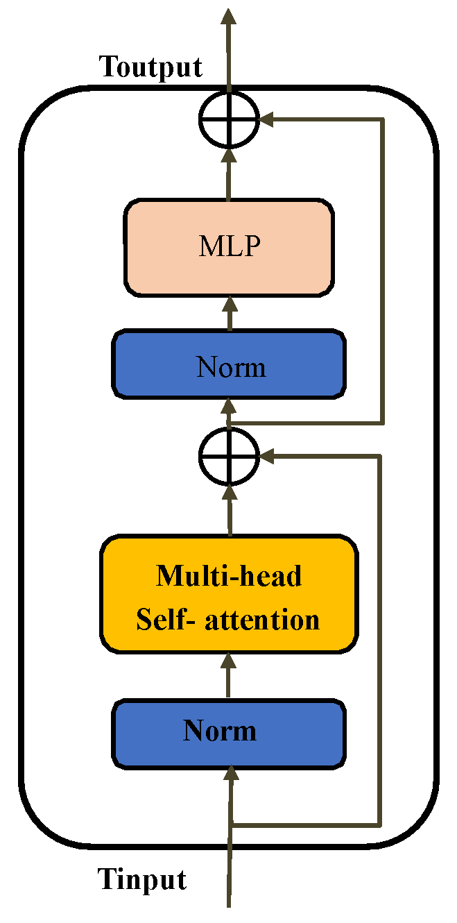
The CNN progressive features extractor are intended to receive further global guidance from the transformer pathway. The convolution operations are used to project the tensor onto a high-dimensional space with 768 channels before the first transformer stage. Therefore, the transformer uses local information of the convolutional layer. This is consistent with the finding that adding locality to the first layers of transformers improves feature representation [60,61]. The CNN’s feature maps are flattened to the size of patches (B × H × W × C) in each step of the transformer, where B denotes the batch size, C the number of channels, and H and W are the height and weight of the feature maps, respectively. As a result, every pixel is treated as an individual PE. The feature maps of spatial dimensions are flattened, and the patch sequence is then fed to the transformer dimension. We now include a trainable class token with these patches. In the typical vision transformer, the final prediction is made using the class token, which is used to collect class-specific data during training [62]. This trainable token is used in the proposed technique along with feature maps in the FFM to offer global features. The TECNN consists of four transformer stages, where a Transformer used a local and global pathway. The global pathway makes a decision on the entire image and the local pathway learns the tumor information form a local patch as shown in Figure 4. In this work we fuse the local and global information to improve the performance. In each stage of transformer, two repeating transformer blocks are used as shown in Figure 5. Each transformer block has multi-layer perceptron (MLP) blocks and multi-head self-attention (MSA) layers, as can be seen Figure 5. Before each MSA and MLP, layer norm is used in this case. In MSA, the input of size B × H × W × C is converted to a query: Q ∈ B × H × W × D q , key K ∈ B × H × W × D q , and value V ∈ B × H × W × D v matrices. Here, C, D q , and DV are the aspects of the input, query matrix, and value matrix, including both. The self-attention is then expressed as follows,
Attention   ( Q ,   K ,   V ) = σ   ( Q K T D v )   V
where σ(·) indicates the SoftMax function. To create the MSA layer, self-attention is carried out head (h) times. There are two adjoining layers in the MLP block, followed by a GELU activation function, where the first layer projects PE to 3072 dimensions and the second layer projects them to 768 dimensions.
The following can be used to express the full procedure in a transformer block.
T o u t p u t M S A = M S A   τ T i n p u t + T i n p u t
T o u t p u t   = MLP   τ T o u t p u t M S A + T o u t p u t M S A
where T o u t p u t M S A   indicates MSL layer output, T o u t p u t   is Transformer blocks output, T i n p u t   is the transformer stage input, and τ(·) is the layer normalization function.

3.3. Feature Merge Module

The FFM connects the transformer and CNN semantically. The feature maps of CNN and transformer PE are different in size, so a direct conversion between them causes a loss of meaningful details.
The FFM receives two inputs, F i n p u t c from CNN and F i n p u t T   from the transformer route. The F i n p u t c has B × C × H × W size, while   F i n p u t T has a size of B × (1 + H × W) × C and 1 for the class token. Before being converted to PE, F i n p u t c is subjected to a global pooling (11 convolutions with BN and ReLU) and has its channel number altered to 768. This GP is viewed as a gate to choose instructive channels and increase the input’s sensitivity to class. The pooled is then down-sampled using average pooling with stride 2. By calculating the average value across adjacent pixels, average pooling can aid in the dissemination of global information. The CNN input is consequently closer to the transformer features. Feature maps are modified to PE F p a t c h C following average pooling. Transformer input ( F i n p u t T ) and output ( F p a t c h C ) are fused to create F o u t p u t T . The proposed model has four FFMs all have F o u t p u t T . As depicted in Figure 6. The output from the previous transformer stage is added to each F o u t p u t T of the FFM, and their sum is input to the following stage. All PE of F i n p u t T , except the class token, are abandoned throughout the fusion process. To obtain F o u t p u t T , F p a t c h C is linked to the class token and local information abounds in F p a t c h C   features, which also assists in CNN transformation. The attention mechanism in Transformer investigates global features on the basis of local feature information to improve the representation capabilities once F o u t p u t T is input to the following transformer stage.
Only the FFM-2 and FFM-4 include the output for the CNN feature extractor, or F o u t p u t c , as seen in Figure 6. Here, IMM-1 and IMM-2 receive F o u t p u t c from FFM -2 and FFM-4. Transformer input ( F i n p u t T ) in the FFM is scaled to the picture space to produce F i m a g e   T . The equation for F o u t p u t c is as follows:
F o u t p u t c = θ ( F i n p u t c )     F i m a g e   T
In this equation the sigmoid function is denoted by θ and the elementwise multiplication is represented by . To give F i m a g e   T appropriate spatial support, the θ ( F i n p u t c ) serves as a mask. Transformer embeddings are turned into the global feature-rich F i m a g e T . Global features that are passed from F i n p u t T to F o u t p u t c can be given to the CNN feature extractor. FFM preserves global features from Transformer pathways and local features from CNN more effectively.

3.4. Intelligent Merge Module

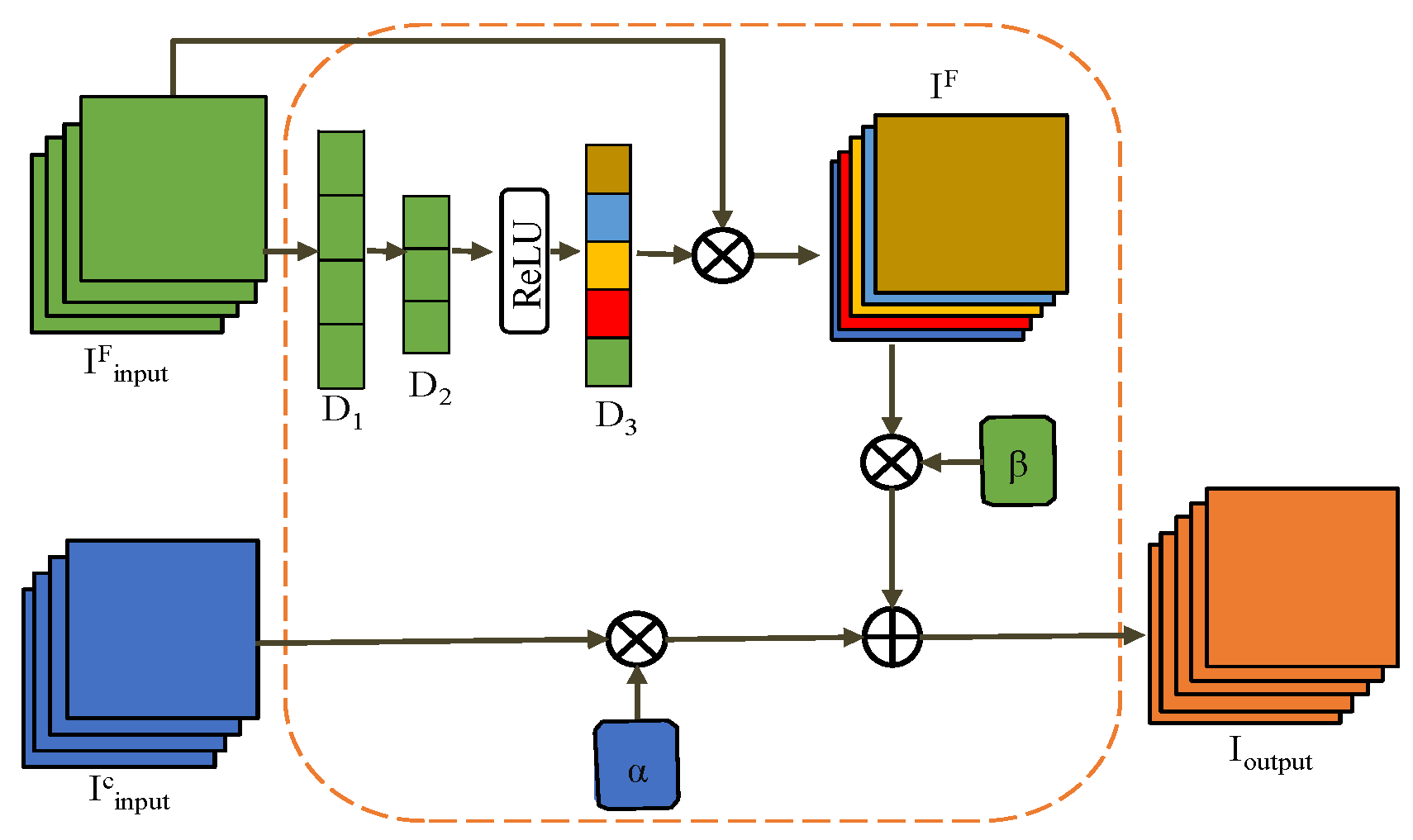
In the IMM, the embeddings of the transformer patch are combined with the CNN features maps and given back to the CNN feature extractor. The IMM makes an effort to make the integration process intelligent so that can gather and choose the most useful data for prediction. The IMM has two inputs, namely I i n p u t c (B × C × H × W) and I i n p u t F (B × C × H × W), as illustrated in Figure 7. I i n p u t c originates from the CNN stage, whereas I o u t p u t F comes from the FFM. There are many global features in I i n p u t F , which is identical to F o u t p u t c of the FFM.
Here, we construct dependencies between the channels of I i n p u t F in order to identify the most useful global characteristics and use these features for aggregation. Figure 7 illustrates how the descriptor D 3   of size, B × C × 1 × 1 reflects these dependencies. C represents the number of channels of I i n p u t F .
Each channel of D 3 only has one pixel, and the value of each pixel indicates the significance of the corresponding channel of I i n p u t F . To accentuate informative channels and reduce less informative channels, I i n p u t F is multiplied by D 3 . Prior to obtaining D 3 , global average pooling is used to combine the spatial information of I i n p u t F and produce descript tor D 1 :
D 1 k = [ i = 1 H   j = 1 W   ( I i n p u t F ) k   ( i ,   j ) ] / H / W
where D 1 and D 3 both have the same size. Here, ( I i n p u t F ) k (i, j) specifies the pixels on the kth channel of I i n p u t F , while D 1 k represents the k-th element of D 1 . A descriptor is obtained and the representation of global features is strengthened by the pooling of global averages. Next, we condense D 1 using a completely connected layer L 1   ,
D 2 = L 1   D 1
where D 2 ∈ B × (C/r) × 1 × 1, r is the compact ratio (set in this study to 16), and another fully linked layer, L 2 , is used to restore the channel number and make use of the data embedded in D 2 once D 2   has passed through a ReLU layer:
D 3 = σ   ( L 2   ( D 2 ) )
where the sigmoid function is represented by σ. In the compact-restore process, the values of the items in D 3 change dynamically during training, and D 3 can pick up on the dependencies between the channels of I i n p u t F . Here, IF is generated by scaling I i n p u t F with D 3 in the manner described below:
I F = I i n p u t F · D 3
Channels that provide more useful information are further highlighted, and the feature representation of IF is enhanced, both of which can be attributed to descriptor D3.
The CNN feature extractor uses the pre-trained model to acquire input C, which includes class-specific data. The input, on the other hand, contains more local features than global feature representations, according to CNN’s fundamental structure. We add these global features to input C via aggregation because IF is transformed from transformer PE and is rich in global features. As a result, the representational power is increased and the proposed TECCN performs better. The output of IMM is the weighted sum of I input C and IF.
( I o u t p u t ) i   = α i . ( I i n p u t C ) i +   β i .   ( I F ) i
where ( I o u t p u t ) i   stands for the feature map on the ith channel of I o u t p u t , ( I i n p u t C ) i and ( I F ) i stand for the ith feature channels of input C and I F , respectively.
In this case, the length of the real number sequences is equal to the number of channels in I i n p u t C . The items in brackets α and β have initial values of 1. The parameters are updated each time an epoch occurs during training, similar to other parameters in the model. α and β determine the weights that the features from I i n p u t C and I F   are contributed, respectively. The aggregate becomes intelligent because of these trainable sequences. I i n p u t C   and I F   have different statistical properties from one another, For instance, there may be significant variations in the mean and variance of pixel count for each channel. Therefore, the mere addition of I i n p u t C and I F can result in the loss of regional or global characteristics. It is possible to determine the proportion of local traits and global characteristics on each feature map so that these two categories simultaneously maintained features. Consequently, the global Transformer features can improve the regional aspects of the CNN and the anticipated TECNN’s representational capacity is enhanced. Furthermore, the proposed model is described in Algorithm 1, which explains the proposed model in a stepwise manner.
Algorithm 1 Training and testing steps of our model provided
Input: Dataset of BT images
Dataset division: Training, Validation, and Testing
Output: Class labels
Training:
Model parameters
  1.
Image size: (224,224,3)
  • P: 9
  • Mini-batch size: 32
  • N; the number of samples
  • Learning rate: 0.0001
  • Optimizer: SGD
  2.
Set the number of mini-batches as: N b = N b
  3.
For iteration = 1: number of epochs
  3.1.
For batch =1 number of mini-batches
  • Online image augmentation during training
  • The obtained training set is fed to the TECCN Convolution and Transformer class branch
  • The augmented images batch is fed to the TECCN encoder of the classification branch
  • The classification token is fed to the token classifier
  • Calculated the loss function
  • Loss backpropagation
  • Updating the model parameters
Model testing:
  1.
Feed the input images to the model
  2.
Calculate the prediction label using output label Y

3.5. Datasets Explanation

Here, we provide a brief explanation of the datasets used in this study, including the BraTS 2018 [63,64] and FIGSHARE datasets, in order to assess the effectiveness of the proposed hybrid model for BT classification.

3.5.1. BraTS 2018 Dataset

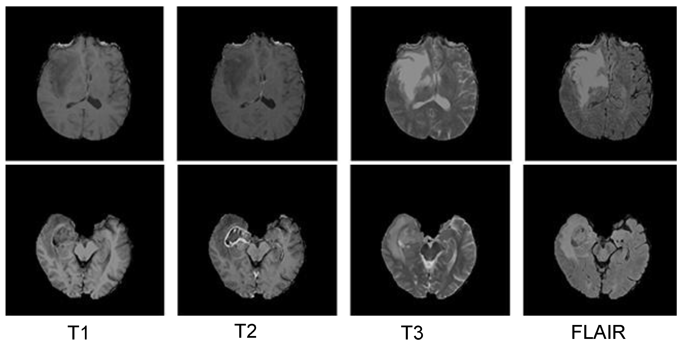
To assess the model’s effectiveness, we choose the BraTS 2018 dataset, which is a commonly used benchmark dataset. This dataset consists of 1425 MRI images, of which 998 MRI images are used for training, 285 MRI images for validation, and 142 MRI images for testing, and included total MRI images of four modalities, those being 356 T1, 355 T2, 356 T1CE, and 358 FLAIR. Sample images of the BraTS 2018 dataset are shown as images in Figure 8.

3.5.2. Figshare Dataset

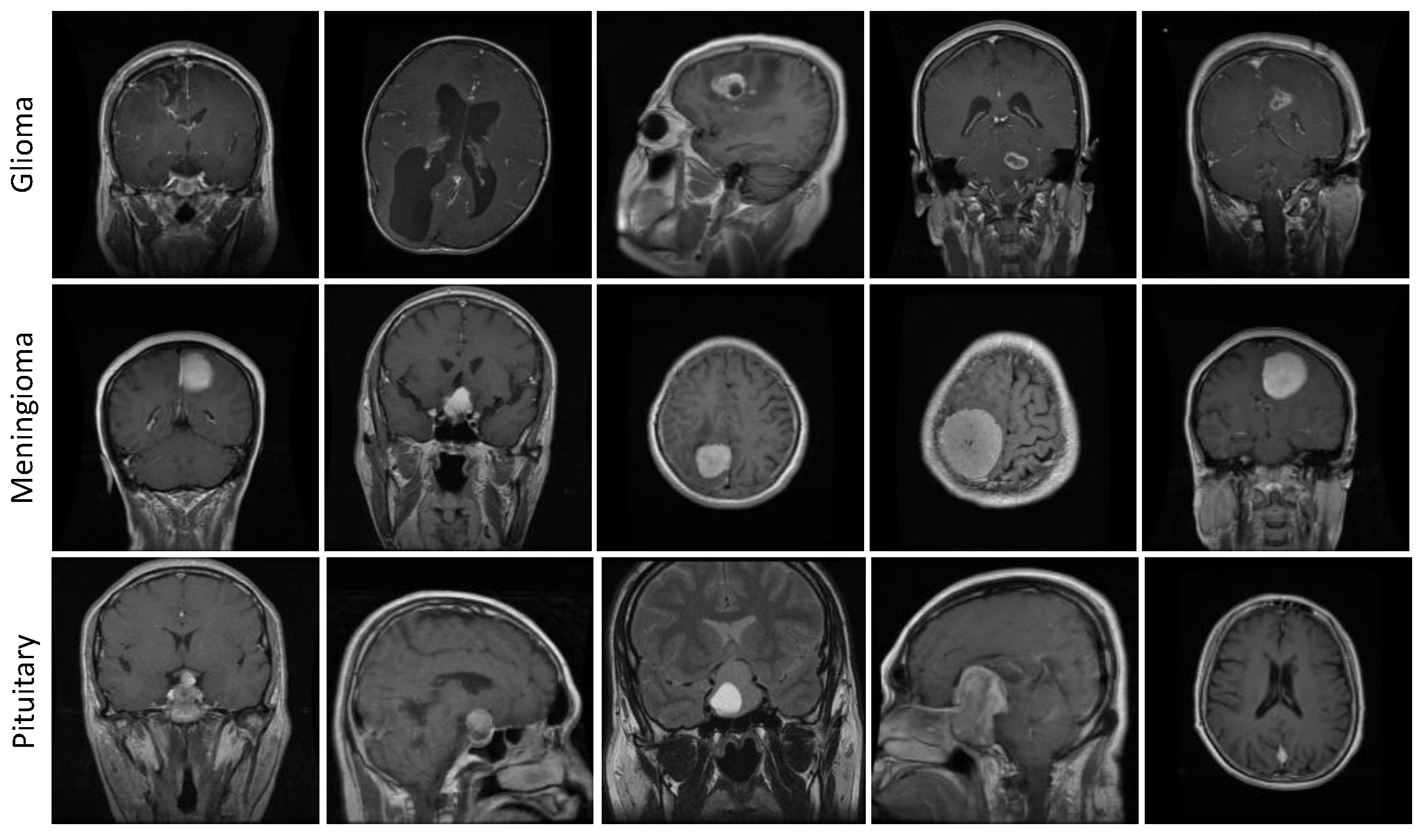
Figshare is a widely used dataset in BT classification research. This dataset was produced by Cheng in 2017 and contains 3064 brain MRI images, including three different types of BT: gliomas, meningiomas, and pituitary. The meningioma class consists of (708 images), glioma (1426 images), and pituitary tumor (930 images). Sample images of the Figshare dataset are presented in Figure 9. We split this dataset into three subgroups: training, validation, and testing, where 70% of the dataset is utilized for training, 20% for validation, and 10% for testing.

4. Results and Discussions

In this work, we perform different experiments for evaluating the model’s effectiveness. This section delivers an explanation of the experimental setup, datasets, evaluation matrices, and provide a detailed discussion of the model outcome analysis (results).

4.1. Training Details

In the experiment, we used 50 epochs to train our model with a low learning rate of 1 × 10⁻⁴, allowing the network to retain the majority of previously acquired knowledge. We trained the proposed model with its 224 × 224 input size, using 32 batch size, and the SGD optimizer with momentum 0.9. For the experimentation, we used NVIDIA GTX 3050 GPU and installed the TensorFlow DL library, and used the Keras DL framework.

4.2. Evaluation Parameters

The effectiveness of our model is assessed on different evaluation parameters precision, recall, F1-measure, and accuracy. The following are the mathematical formulation of these matrices.
Accuracy = ( TP + TN TP + TN + FP + FN )
Precision = ( TP TP + FP )
recall = ( TP TP + FN )
F 1 score = 2 ( precision recall precision + recall )
where TP indicates a true positive, TN is a true negative, FP is a false positive, and FN false negative.

4.3. Results Evaluation Using BraTS 2018 Dataset

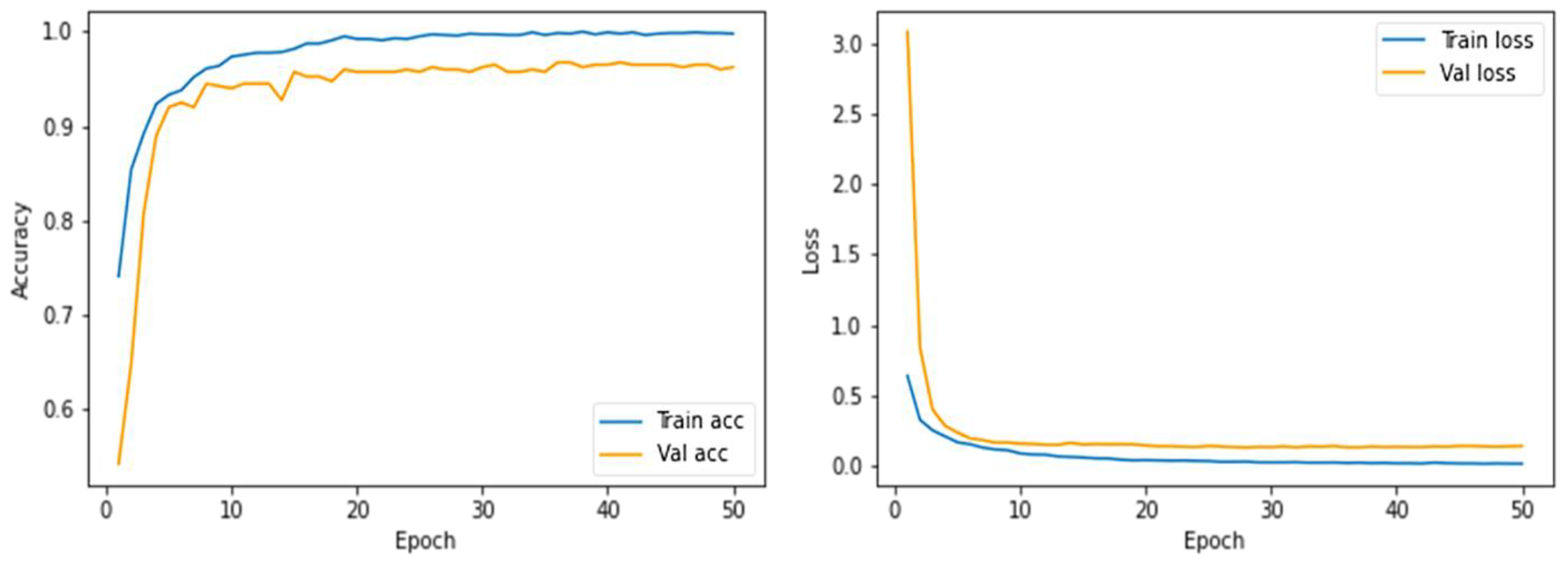
The model is trained in the experiments using an SGD optimizer over the course of 50 epochs. The training and validation accuracy curves are steadily improving after each epoch, as shown in Figure 10. Our model reaches 96.75% and 97.50% for training and validation accuracy, respectively, on the 15 epochs.
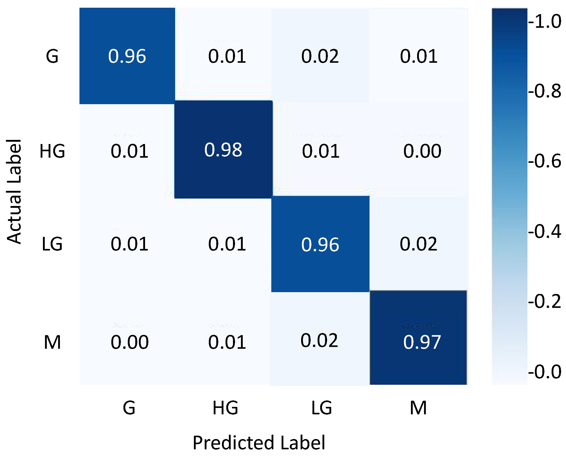
The classification report of our model using testing set is shown in Table 1. The proposed model effectively classifies BT such as G (glioma) with a ratio of 96%, HG (high-grade glioma) with 98%, LG (Low-grade glioma) with 96%, and M (meningioma) with 97% as shown in Table 1, which demonstrates the effectiveness of our model using the BraTS 2018 dataset. The proposed model confusion matrix using the BraTS 2018 dataset is provided in Figure 11, where the ratio of positive predicted samples is high for each category.
The proposed model is compared with four different state-of-the-art models DR LBP features + k–NN [65], Inception V3 + SVM [65], PSO features + Softmax [65], and Two-Channel DNN [66], as given in Table 2. In the comparison, the DR LBP features + k–NN obtain 85.10% accuracy, which is the lowest in this experiment. The proposed model surpasses the DR LBP features + k–NN by achieving 11.65% higher accuracy. The Inception V3 + SVM, PSO features + Softmax, and Two-Channel DNN achieve accuracy of 87.40, 92.50, and 93.69, respectively. The proposed model surpasses Inception V3 + SVM, PSO features + Softmax, and Two-Channel DNN by obtaining 9.35%, 4.25%, and 3.36% higher accuracy, respectively. The accuracy of our models is 96.75%, which is higher than other models. Our model is able to perform at a level that is superior to that of the other models.

4.4. Results Evaluation Using Figshare Dataset

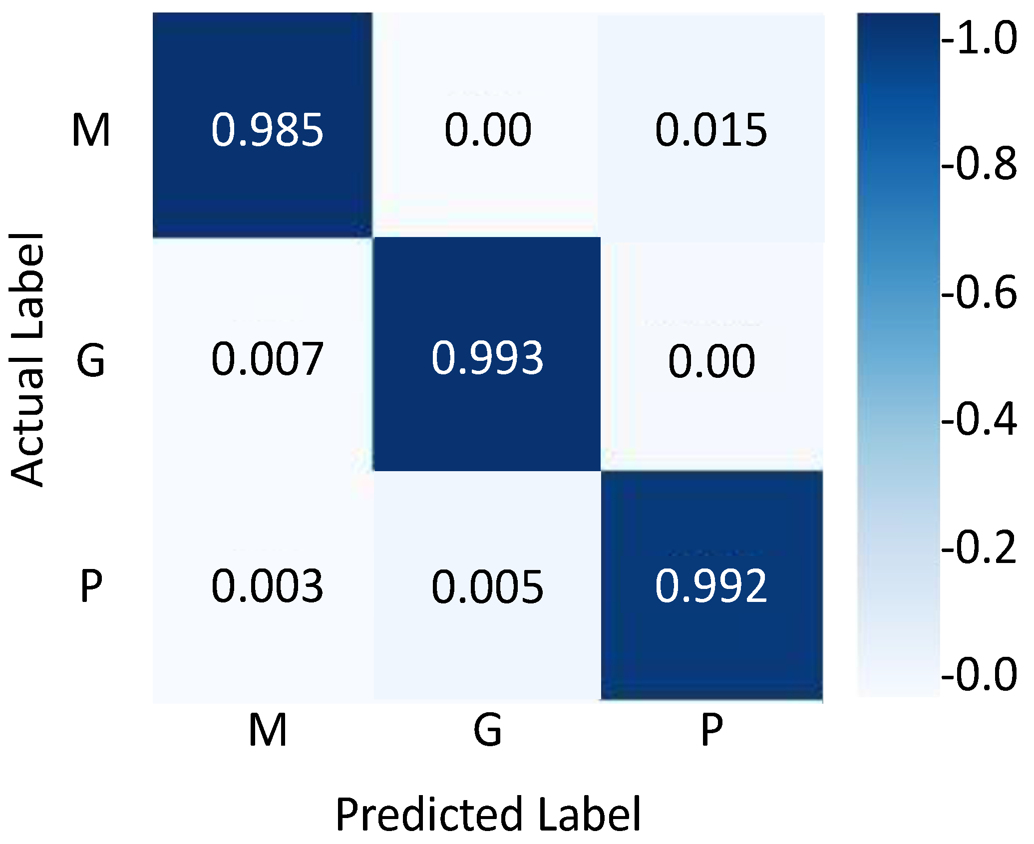
The training and validation accuracies can be seen in Figure 12. Table 3 provides the classification report of our model using a FIGSHARE dataset. Figure 13 provides confusion matrix using a FIGSHARE dataset. Table 4 presents comparison results of our proposed model with the state-of-the-art models. Our model is successfully trained and validated across a total of 50 epochs, with an accuracy level reaches 99%.
Table 4 provides a summary of the past studies as well as scores indicating their accuracy for BT classification. Studies for the categorization of brain cancers included feature extraction methods such as Fisher Vector, GLCM, Bag of words, and DSURF/HoG [67,68,69,70] are provided. In addition, the SVM classifier is utilized in each of these experiments. Cheng et al. [28] that is based on more conventional approaches, achieves the highest accuracy score (94.68%) of all of compared works.
However, deep feature extraction and transfer learning are applied in the research that relied on pre-trained deep architectures studies that employed a deep feature extraction strategy offered a hybrid of pre-trained deep models and SVM/ELM/Softmax classifiers [66,71,72] Among these investigations, the results from Türkoğlu M et al. [73] show the highest accuracy, at 98.04%. (2021).
The transfer learning strategy [74,75] using AlexNet and VGG19, respectively by Swati et al. [74] and Kaur and Gandhi’s [75], where the [75] achieved the highest accuracy. The deep learning model to classify BT was shown superior results to those using traditional ML models, as shown in Table 4. However, our hybrid model achieved the highest accuracy as compared with traditional ML and deep learning-based models.
Table 4. Comparison of the proposed model with the state-of-the-art methods using the FIGSHARE dataset.
ReferencesAccuracy
Ari et al. [72]97.64%
Cheng et al. [28]94.68%
Abir et al. [69]83.33%
Afshar et al. [76]86.56%
Cheng et al. [67]91.28%
Deepak and Ameer [71]97.10%
Kaur and Gandhi [75]96.95%
Ayadi et al. [77]90.27%
Pashaei et al. [78] 93.68%
Swati et al. [74]94.80%
Deepak and Ameer [79]95.82%
Bodapati et al. [66]95.23%
Türkoğlu M et al. [73].98.04%
Proposed Model99.10%

4.5. Comparing the Proposed Model with Various CNN and ViT-Based Models

In this subsection, we compare the results of our model with various types of CNNs and ViT models to evaluate the model effectiveness. In consideration, the proposed model is compared with Solo AlexNet, Inception V3, VGG19, ResNet50, and ViT using BraTS 2018 and FIGSHARE datasets as presented in Table 5. The proposed model obtains higher accuracy compared to other models using BraTS 2018 and FIGSHARE. In comparison, the proposed model is efficient in terms of learning parameters of 22.5 million. Thus, the proposed model is an efficient and effective solution for brain tumor classification as proven by these experimental results.
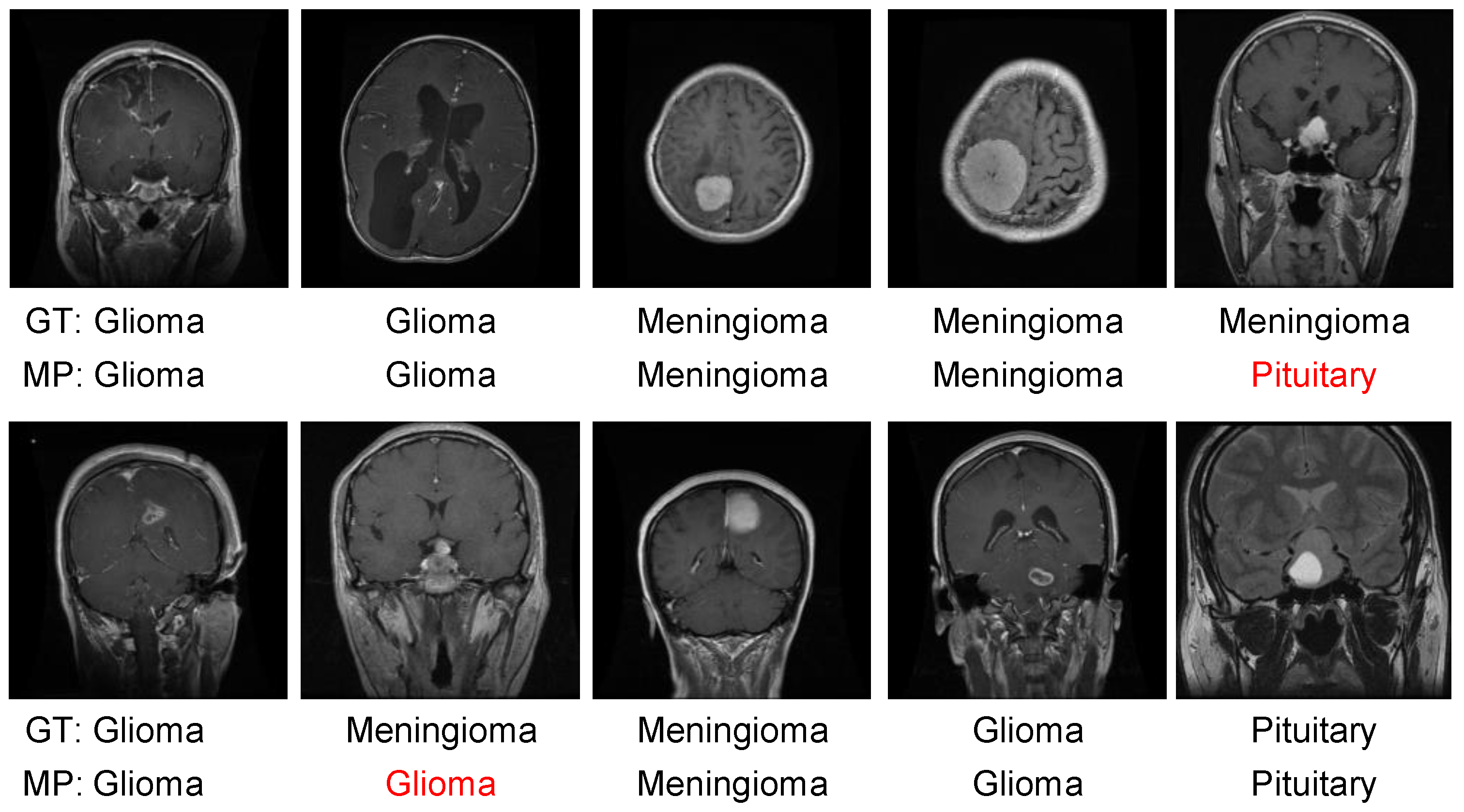
The visual result of the proposed model is demonstrated in Figure 14, where the GT indicates the ground truth and MP represents model prediction. It can be seen that the proposed model is confused in the prediction of two samples. Our model misclassifies the last image of the first row and the second image of the second row as shown in Figure 14 with red color. We believe that this misprediction is due to the visual similarity with other classes.

5. Conclusions

In this paper, we proposed a novel hybrid deep learning-based model for BT classification. The proposed model integrated the transformer and CNNs to achieve the capabilities of both networks. Furthermore, to achieve more desirable results we used the FFM and IMM, which increase the feature representation capability. The proposed model evaluated using two publicly available datasets, and the experimental results showed the effectiveness of the proposed model, in helping the radiologist in taking a precise decision for classifying BT. Our model achieved a competitive accuracy of 96.75% and 99.10% on BRATS’2018 and FIGSHARE datasets, respectively, which proved the model’s superiority over state-of-the-art models.
In the future, we aim to extend our current work for fine-grained classification of each grade with the investigation of a lightweight CNN model to balance efficiency and accuracy.

Author Contributions

Conceptualization, M.A.; Methodology, A.K.; Software, S.A.; M.I. and M.F.A.; Validation, S.H.; Formal analysis, S.A. and S.H.; Investigation, M.F.A.; Resources, S.H.; Data curation, S.A. and M.F.A.; Writing—original draft, M.A.; M.I and A.K.; Writing—review and editing, A.K.; Visualization, M.A.; Supervision, M.I.; Project administration, M.I.; Funding acquisition, M.A. All authors have read and agreed to the published version of the manuscript.

Funding

This research received no external funding.

Institutional Review Board Statement

Not applicable.

Informed Consent Statement

Not applicable.

Data Availability Statement

Not applicable.

Acknowledgments

Researchers would like to thank the Deanship of Scientific Research, Qassim University for funding publication of this project.

Conflicts of Interest

The authors declare no conflict of interest.

References

  1. Zhao, L.; Jia, K. Multiscale CNNs for brain tumor segmentation and diagnosis. Comput. Math. Methods Med. 2016, 2016, 8356294. [Google Scholar] [CrossRef] [PubMed] [Green Version]
  2. Rajinikanth, V.; Fernandes, S.L.; Bhushan, B.; Harisha; Sunder, N.R. Segmentation and analysis of brain tumor using Tsallis entropy and regularised level set. In Proceedings of the 2nd International Conference on Micro-Electronics, Electromagnetics and Telecommunications, Ghaziabad, India, 20–21 September 2018. [Google Scholar]
  3. Cancer Research UK. Together We Will Beat Cancer; Cancer Research UK: London, UK. Available online: https://fundraise.cancerresearchuk.org/page/together-we-will-beat-cancer (accessed on 13 December 2022).
  4. Sajjad, M.; Khan, S.; Muhammad, K.; Wu, W.; Ullah, A.; Baik, S.W. Multi-grade brain tumor classification using deep CNN with extensive data augmentation. J. Comput. Sci. 2019, 30, 174–182. [Google Scholar] [CrossRef]
  5. Varuna Shree, N.; Kumar, T. Identification and classification of brain tumor MRI images with feature extraction using DWT and probabilistic neural network. Brain Inform. 2018, 5, 23–30. [Google Scholar] [CrossRef] [PubMed] [Green Version]
  6. Zeng, K.; Zheng, H.; Cai, C.; Yang, Y.; Zhang, K.; Chen, Z. Simultaneous single-and multi-contrast super-resolution for brain MRI images based on a convolutional neural network. Comput. Biol. Med. 2018, 99, 133–141. [Google Scholar] [CrossRef] [PubMed]
  7. Mittal, M.; Goyal, L.M.; Kaur, S.; Kaur, I.; Verma, A.; Hemanth, D.J. Deep learning based enhanced tumor segmentation approach for MR brain images. Appl. Soft Comput. 2019, 78, 346–354. [Google Scholar] [CrossRef]
  8. Bunevicius, A.; Schregel, K.; Sinkus, R.; Golby, A.; Patz, S. MR elastography of brain tumors. NeuroImage Clin. 2020, 25, 102109. [Google Scholar] [CrossRef] [PubMed]
  9. Khan, M.A.; Ashraf, I.; Alhaisoni, M.; Damaševičius, R.; Scherer, R.; Rehman, A.; Bukhari, S. Multimodal brain tumor classification using deep learning and robust feature selection: A machine learning application for radiologists. Diagnostics 2020, 10, 565. [Google Scholar] [CrossRef]
  10. Iqbal, S.; Ghani, M.U.; Saba, T.; Rehman, A. Brain tumor segmentation in multi-spectral MRI using convolutional neural networks (CNN). Microsc. Res. Tech. 2018, 81, 419–427. [Google Scholar] [CrossRef]
  11. Arakeri, M.P.; Reddy, G. Computer-aided diagnosis system for tissue characterization of brain tumor on magnetic resonance images. Signal Image Video Process. 2013, 9, 409–425. [Google Scholar] [CrossRef]
  12. Usman, K.; Rajpoot, K. Brain tumor classification from multi-modality MRI using wavelets and machine learning. Pattern Anal. Appl. 2017, 20, 871–881. [Google Scholar] [CrossRef] [Green Version]
  13. Mohsen, H.; El-Dahshan, E.-S.A.; El-Horbaty, E.-S.M.; Salem, A.-B.M. Classification using deep learning neural networks for brain tumors. Future Comput. Inform. J. 2018, 3, 68–71. [Google Scholar] [CrossRef]
  14. Habib, S.; Alyahya, S.; Ahmed, A.; Islam, M.; Khan, S.; Khan, I.; Kamil, M. X-ray Image-Based COVID-19 Patient Detection Using Machine Learning-Based Techniques. Comput. Syst. Sci. Eng. 2022, 43, 671–682. [Google Scholar] [CrossRef]
  15. Yar, H.; Hussain, T.; Khan, Z.A.; Koundal, D.; Lee, M.Y.; Baik, S.W. Vision sensor-based real-time fire detection in resource-constrained IoT environments. Comput. Intell. Neurosci. 2021, 2021, 5195508. [Google Scholar] [CrossRef]
  16. Yar, H.; Hussain, T.; Agarwal, M.; Khan, Z.A.; Gupta, S.K.; Baik, S.W. Optimized Dual Fire Attention Network and Medium-Scale Fire Classification Benchmark. IEEE Trans. Image Process. 2022, 31, 6331–6343. [Google Scholar] [CrossRef] [PubMed]
  17. Ullah, W.; Hussain, T.; Khan, Z.A.; Haroon, U.; Baik, S.W. Intelligent dual stream CNN and echo state network for anomaly detection. Knowl.-Based Syst. 2022, 253, 109456. [Google Scholar] [CrossRef]
  18. Habib, S.; Alsanea, M.; Aloraini, M.; Al-Rawashdeh, H.S.; Islam, M.; Khan, S. An Efficient and Effective Deep Learning-Based Model for Real-Time Face Mask Detection. Sensors 2022, 22, 2602. [Google Scholar] [CrossRef]
  19. Khan, Z.A.; Hussain, T.; Haq, I.U.; Ullah, F.U.M.; Baik, S.W. Towards efficient and effective renewable energy prediction via deep learning. Energy Rep. 2022, 8, 10230–10243. [Google Scholar] [CrossRef]
  20. Khan, Z.A.; Hussain, T.; Baik, S. Boosting energy harvesting via deep learning-based renewable power generation prediction. J. King Saud Univ.-Sci. 2022, 34, 101815. [Google Scholar] [CrossRef]
  21. Albattah, W.; Kaka Khel, M.H.; Habib, S.; Islam, M.; Khan, S.; Abdul Kadir, K. Hajj Crowd Management Using CNN-Based Approach. Comput. Mater. Contin. 2020, 66, 2183–2197. [Google Scholar] [CrossRef]
  22. Khan, Z.A.; Hussain, T.; Ullah, F.U.M.; Gupta, S.K.; Lee, M.Y.; Baik, S.W. Randomly Initialized CNN with Densely Connected Stacked Autoencoder for Efficient Fire Detection. Eng. Appl. Artif. Intell. 2022, 116, 105403. [Google Scholar] [CrossRef]
  23. Seetha, J.; Raja, S. Brain Tumor Classification Using Convolutional Neural Networks. Biomed. Pharmacol. J. 2018, 11, 1457–1461. [Google Scholar] [CrossRef]
  24. Habib, S.; Hussain, A.; Albattah, W.; Islam, M.; Khan, S.; Khan, R.U.; Khan, K. Abnormal Activity Recognition from Surveillance Videos Using Convolutional Neural Network. Sensors 2021, 21, 8291. [Google Scholar] [CrossRef] [PubMed]
  25. Khan, K.; Khan, R.U.; Albattah, W.; Nayab, D.; Qamar, A.M.; Habib, S.; Islam, M. Crowd Counting Using End-to-End Semantic Image Segmentation. Electronics 2021, 10, 1293. [Google Scholar] [CrossRef]
  26. Ullah, R.; Hayat, H.; Siddiqui, A.A.; Siddiqui, U.A.; Khan, J.; Ullah, F.; Hassan, S.; Hasan, L.; Albattah, W.; Islam, M.; et al. A real-time framework for human face detection and recognition in cctv images. Math. Probl. Eng. 2022, 2022, 3276704. [Google Scholar] [CrossRef]
  27. Amin, J.; Sharif, M.; Yasmin, M.; Saba, T.; Anjum, M.A.; Fernandes, S.L. A New Approach for Brain Tumor Segmentation and Classification Based on Score Level Fusion Using Transfer Learning. J. Med. Syst. 2019, 43, 326. [Google Scholar] [CrossRef] [PubMed]
  28. Dosovitskiy, A.; Beyer, L.; Kolesnikov, A.; Weissenborn, D.; Zhai, X.; Unterthiner, T.; Dehghani, M.; Minderer, M.; Heigold, G.; Gelly, S.; et al. An image is worth 16x16 words: Transformers for image recognition at scale. arXiv 2020, arXiv:2010.11929. [Google Scholar]
  29. Chen, S.; Li, W.; Cao, Y.; Lu, X. Combining the Convolution and Transformer for Classification of Smoke-Like Scenes in Remote Sensing Images. IEEE Trans. Geosci. Remote Sens. 2022, 60, 4512519. [Google Scholar] [CrossRef]
  30. Yar, H.; Abbas, N.; Sadad, T.; Iqbal, S. Lung nodule detection and classification using 2D and 3D convolution neural networks (CNNs). In Artificial Intelligence and Internet of Things; CRC Press: Boca Raton, FL, USA, 2021; pp. 365–386. [Google Scholar] [CrossRef]
  31. Awan, M.J.; Rahim, M.S.M.; Salim, N.; Rehman, A.; Garcia-Zapirain, B. Automated knee MR images segmentation of anterior cruciate ligament tears. Sensors 2022, 22, 1552. [Google Scholar] [CrossRef]
  32. Alyami, J.; Rehman, A.; Sadad, T.; Alruwaythi, M.; Saba, T.; Bahaj, S.A. Automatic skin lesions detection from images through microscopic hybrid features set and machine learning classifiers. Microsc. Res. Tech. 2022, 85, 3600–3607. [Google Scholar] [CrossRef]
  33. Gull, S.; Akbar, S.; Hassan, S.A.; Rehman, A.; Sadad, T. Automated Brain Tumor Segmentation and Classification Through MRI Images. In Proceedings of the International Conference on Emerging Technology Trends in Internet of Things and Computing, Erbil, Iraq, 6–8 June 2021; Springer: Cham, Switzerland, 2022. [Google Scholar]
  34. Ayesha, H.; Iqbal, S.; Tariq, M.; Abrar, M.; Sanaullah, M.; Abbas, I.; Rehman, A.; Niazi, M.F.K.; Hussain, S. Automatic medical image interpretation: State of the art and future directions. Pattern Recognit. 2021, 114, 107856. [Google Scholar] [CrossRef]
  35. Talo, M.; Baloglu, U.B.; Yıldırım, Ö.; Acharya, U.R. Application of deep transfer learning for automated brain abnormality classification using MR images. Cogn. Syst. Res. 2019, 54, 176–188. [Google Scholar] [CrossRef]
  36. Rehman, A.; Naz, S.; Razzak, M.I.; Akram, F.; Imran, M. A Deep Learning-Based Framework for Automatic Brain Tumors Classification Using Transfer Learning. Circuits Syst. Signal Process. 2019, 39, 757–775. [Google Scholar] [CrossRef]
  37. Mehrotra, R.; Ansari, M.; Agrawal, R.; Anand, R. A Transfer Learning approach for AI-based classification of brain tumors. Mach. Learn. Appl. 2020, 2, 100003. [Google Scholar] [CrossRef]
  38. Khan, H.A.; Jue, W.; Mushtaq, M.; Mushtaq, M.U. Brain tumor classification in MRI image using convolutional neural network. Math. Biosci. Eng. 2020, 17, 6203–6216. [Google Scholar] [CrossRef]
  39. Ayadi, W.; Elhamzi, W.; Charfi, I.; Atri, M. Deep CNN for Brain Tumor Classification. Neural Process. Lett. 2021, 53, 671–700. [Google Scholar] [CrossRef]
  40. Pereira, S.; Meier, R.; Alves, V.; Reyes, M.; Silva, C.A. Automatic brain tumor grading from MRI data using convolutional neural networks and quality assessment. In Understanding and Interpreting Machine Learning in Medical Image Computing Applications; Springer: Cham, Switzerland, 2018; pp. 106–114. [Google Scholar]
  41. Farman, H.; Khan, T.; Khan, Z.; Habib, S.; Islam, M.; Ammar, A. Real-Time Face Mask Detection to Ensure COVID-19 Precautionary Measures in the Developing Countries. Appl. Sci. 2022, 12, 3879. [Google Scholar] [CrossRef]
  42. Jude Hemanth, D.; Vijila, C.S.; Selvakumar, A.; Anitha, J. Performance Improved Iteration-Free Artificial Neural Networks for Abnormal Magnetic Resonance Brain Image Classification. Neurocomputing 2014, 130, 98–107. [Google Scholar] [CrossRef]
  43. Abiwinanda, N.; Hanif, M.; Hesaputra, S.T.; Handayani, A.; Mengko, T.R. Brain Tumor Classification Using Convolutional Neural Network. In Proceedings of the World Congress on Medical Physics and Biomedical Engineering, Prague, Czech Republic, 3–8 June 2018; pp. 183–189. [Google Scholar]
  44. Zhou, Y.; Li, Z.; Zhu, H.; Chen, C.; Gao, M.; Xu, K.; Xu, J. Holistic brain tumor screening and classification based on densenet and recurrent neural network. In Proceedings of the International MICCAI Brainlesion Workshop, Granada, Spain, 16 September 2018. [Google Scholar]
  45. Afshar, P.; Mohammadi, A.; Plataniotis, K.N.; Oikonomou, A.; Benali, H. From handcrafted to deep-learning-based cancer radiomics: Challenges and opportunities. IEEE Signal Process. Mag. 2019, 36, 132–160. [Google Scholar] [CrossRef] [Green Version]
  46. Sharif, M.I.; Khan, M.A.; Alhussein, M.; Aurangzeb, K.; Raza, M. A decision support system for multimodal brain tumor classification using deep learning. Complex Intell. Syst. 2021, 8, 3007–3020. [Google Scholar] [CrossRef]
  47. Sekhar, A.; Biswas, S.; Hazra, R.; Sunaniya, A.K.; Mukherjee, A.; Yang, L. Brain tumor classification using fine-tuned GoogLeNet features and machine learning algorithms: IoMT enabled CAD system. IEEE J. Biomed. Health Inform. 2021, 26, 983–991. [Google Scholar] [CrossRef] [PubMed]
  48. Abbood, A.A.; Shallal, Q.; Fadhel, M. Automated brain tumor classification using various deep learning models: A comparative study. Indones. J. Electr. Eng. Comput. Sci. 2021, 22, 252. [Google Scholar] [CrossRef]
  49. Tummala, S.; Kadry, S.; Bukhari, S.A.C.; Rauf, H.T. Classification of Brain Tumor from Magnetic Resonance Imaging Using Vision Transformers Ensembling. Curr. Oncol. 2022, 29, 7498–7511. [Google Scholar] [CrossRef] [PubMed]
  50. Xu, X.; Prasanna, P. Brain Cancer Survival Prediction on Treatment-Naïve MRI using Deep Anchor Attention Learning with Vision Transformer. In Proceedings of the 2022 IEEE 19th International Symposium on Biomedical Imaging (ISBI), Kolkata, India, 28–31 March 2022. [Google Scholar]
  51. Nallamolu, S.; Nandanwar, H.; Singh, A.; Subalalitha, C.N. A CNN-based Approach for Multi-Classification of Brain Tumors. In Proceedings of the 2022 2nd Asian Conference on Innovation in Technology (ASIANCON), Ravet, India, 26–28 August 2022. [Google Scholar]
  52. Aladhadh, S.; Alsanea, M.; Aloraini, M.; Khan, T.; Habib, S.; Islam, M. An Effective Skin Cancer Classification Mechanism via Medical Vision Transformer. Sensors 2022, 22, 4008. [Google Scholar] [CrossRef]
  53. Hatamizadeh, A.; Nath, V.; Tang, Y.; Yang, D.; Roth, H.R.; Xu, D. Swin unetr: Swin transformers for semantic segmentation of brain tumors in mri images. In Proceedings of the International MICCAI Brainlesion Workshop, Virtual Event, 27 September 2021. [Google Scholar]
  54. Jiang, Y.; Zhang, Y.; Lin, X.; Dong, J.; Cheng, T.; Liang, J. SwinBTS: A method for 3D multimodal brain tumor segmentation using swin transformer. Brain Sci. 2022, 12, 797. [Google Scholar] [CrossRef]
  55. Gai, D.; Zhang, J.; Xiao, Y.; Min, W.; Zhong, Y.; Zhong, Y. RMTF-Net: Residual Mix Transformer Fusion Net for 2D Brain Tumor Segmentation. Brain Sci. 2022, 12, 1145. [Google Scholar] [CrossRef]
  56. Peng, Z.; Huang, W.; Gu, S.; Xie, L.; Wang, Y.; Jiao, J.; Ye, Q. Conformer: Local features coupling global representations for visual recognition. In Proceedings of the IEEE/CVF International Conference on Computer Vision, Montreal, QC, Canada, 11–17 October 2021. [Google Scholar]
  57. Lu, X.; Sun, H.; Zheng, X. A feature aggregation convolutional neural network for remote sensing scene classification. IEEE Trans. Geosci. Remote Sens. 2019, 57, 7894–7906. [Google Scholar] [CrossRef]
  58. Deng, J.; Dong, W.; Socher, R.; Li, L.J.; Li, K.; Fei-Fei, L. Imagenet: A large-scale hierarchical image database. In Proceedings of the 2009 IEEE Conference on Computer Vision and Pattern Recognition, Miami, FL, USA, 20–25 June 2009. [Google Scholar]
  59. Huang, G.; Liu, Z.; Van Der Maaten, L.; Weinberger, K.Q. Densely connected convolutional networks. In Proceedings of the IEEE Conference on Computer Vision and Pattern Recognition, Honolulu, HI, USA, 21–26 July 2017. [Google Scholar]
  60. Dai, Z.; Liu, H.; Le, Q.V.; Tan, M. Coatnet: Marrying convolution and attention for all data sizes. Adv. Neural Inf. Process. Syst. 2021, 34, 3965–3977. [Google Scholar]
  61. Aladhadh, S.; Almatroodi, S.A.; Habib, S.; Alabdulatif, A.; Khattak, S.U.; Islam, M. An Efficient Lightweight Hybrid Model with Attention Mechanism for Enhancer Sequence Recognition. Biomolecules 2023, 13, 70. [Google Scholar] [CrossRef]
  62. Yar, H.; Hussain, T.; Khan, Z.A.; Lee, M.Y.; Baik, S.W. Fire Detection via Effective Vision Transformers. J. Korean Inst. Next Gener. Comput. 2021, 17, 21–30. [Google Scholar]
  63. Gull, S.; Akbar, S.; Khan, H. Automated detection of brain tumor through magnetic resonance images using convolutional neural network. BioMed Res. Int. 2021, 2021, 3365043. [Google Scholar] [CrossRef]
  64. Abd El Kader, I.; Xu, G.; Shuai, Z.; Saminu, S.; Javaid, I.; Ahmad, I.S. Differential deep convolutional neural network model for brain tumor classification. Brain Sci. 2021, 11, 352. [Google Scholar] [CrossRef]
  65. Sharif, M.I.; Li, J.P.; Khan, M.A.; Saleem, M.A. Active deep neural network features selection for segmentation and recognition of brain tumors using MRI images. Pattern Recognit. Lett. 2020, 129, 181–189. [Google Scholar] [CrossRef]
  66. Bodapati, J.D.; Shaik, N.S.; Naralasetti, V.; Mundukur, N.B. Joint training of two-channel deep neural network for brain tumor classification. Signal Image Video Process. 2021, 15, 753–760. [Google Scholar] [CrossRef]
  67. Cheng, J.; Huang, W.; Cao, S.; Yang, R.; Yang, W.; Yun, Z.; Wang, Z.; Feng, Q. Enhanced Performance of Brain Tumor Classification via Tumor Region Augmentation and Partition. PLoS ONE 2015, 10, e0140381. [Google Scholar] [CrossRef]
  68. Cheng, J.; Yang, W.; Huang, M.; Huang, W.; Jiang, J.; Zhou, Y.; Yang, R.; Zhao, J.; Feng, Y.; Feng, Q.; et al. Retrieval of Brain Tumors by Adaptive Spatial Pooling and Fisher Vector Representation. PLoS ONE 2016, 11, e0157112. [Google Scholar] [CrossRef] [PubMed] [Green Version]
  69. Abir, T.A.; Siraji, J.A.; Ahmed, E.; Khulna, B. Analysis of a novel MRI based brain tumour classification using probabilistic neural network (PNN). Int. J. Sci. Res. Sci. Eng. Technol 2018, 4, 65–79. [Google Scholar]
  70. Hossain, A.; Islam, M.T.; Abdul Rahim, S.K.; Rahman, M.A.; Rahman, T.; Arshad, H.; Khandakar, A.; Ayari, M.A.; Chowdhury, M.E.H. A Lightweight Deep Learning Based Microwave Brain Image Network Model for Brain Tumor Classification Using Reconstructed Microwave Brain (RMB) Images. Biosensors 2023, 13, 238. [Google Scholar] [CrossRef] [PubMed]
  71. Deepak, S.; Ameer, P. Brain tumor classification using deep CNN features via transfer learning. Comput. Biol. Med. 2019, 111, 103345. [Google Scholar] [CrossRef]
  72. Arı, A.; Alcin, O.; Hanbay, D. Brain MR image classification based on deep features by using extreme learning machines. Biomed. J. Sci. Tech. Res. 2020, 25. [Google Scholar] [CrossRef]
  73. Türkoğlu, M. Brain Tumor Detection using a combination of Bayesian optimization based SVM classifier and fine-tuned based deep features. Avrupa Bilim Teknol. Derg. 2021, 27, 251–258. [Google Scholar] [CrossRef]
  74. Swati, Z.N.K.; Zhao, Q.; Kabir, M.; Ali, F.; Ali, Z.; Ahmed, S.; Lu, J. Brain tumor classification for MR images using transfer learning and fine-tuning. Comput. Med. Imaging Graph. 2019, 75, 34–46. [Google Scholar] [CrossRef] [PubMed]
  75. Kaur, T.; Gandhi, T.K. Deep convolutional neural networks with transfer learning for automated brain image classification. Mach. Vis. Appl. 2020, 31, 20. [Google Scholar] [CrossRef]
  76. Alsanea, M.; Dukyil, A.S.; Afnan; Riaz, B.; Alebeisat, F.; Islam, M.; Habib, S. To Assist Oncologists: An Efficient Machine Learning-Based Approach for Anti-Cancer Peptides Classification. Sensors 2022, 22, 4005. [Google Scholar] [CrossRef] [PubMed]
  77. Ayadi, W.; Charfi, I.; Elhamzi, W.; Atri, M. Brain tumor classification based on hybrid approach. Vis. Comput. 2020, 38, 107–117. [Google Scholar] [CrossRef]
  78. Pashaei, A.; Sajedi, H.; Jazayeri, N. Brain tumor classification via convolutional neural network and extreme learning machines. In Proceedings of the 2018 8th International Conference on Computer and Knowledge Engineering (ICCKE), Mashhad, Iran, 25–26 October 2018. [Google Scholar]
  79. Deepak, S.; Ameer, P. Automated categorization of brain tumor from mri using cnn features and svm. J. Ambient Intell. Humaniz. Comput. 2021, 12, 8357–8369. [Google Scholar] [CrossRef]
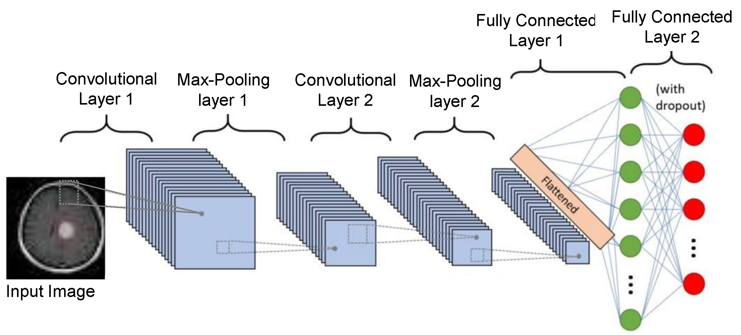
Figure 1. Represents the overall structure of a basic CNN.
Applsci 13 03680 g001
Figure 4. Represents the Transformer Pathway for collecting local and global features.
Applsci 13 03680 g004
Figure 5. Transformer block structure.
Applsci 13 03680 g005
Figure 6. The proposed FFM structure.
Applsci 13 03680 g006
Figure 7. Representation of the IMM structure.
Applsci 13 03680 g007
Figure 8. Sample images of the BraTS 2018 dataset.
Applsci 13 03680 g008
Figure 9. Sample images of Figshare for BT classification.
Applsci 13 03680 g009
Figure 10. Training-validation accuracy and loss curves of our model using BRATS 2018 dataset.
Applsci 13 03680 g010
Figure 11. Confusion matrix of the proposed model using BRATS’2018 dataset.
Applsci 13 03680 g011
Figure 12. Training-validation accuracy and loss curves of our model using the FIGSHARE dataset.
Applsci 13 03680 g012
Figure 13. Confusion matrix of the proposed model using FIGSHARE datasets, where M represents Meningiomas, G Gliomas, and P Pituitary tumors.
Applsci 13 03680 g013
Figure 14. The visualized result of the proposed model.
Applsci 13 03680 g014
Table 1. Classification report of our model using BRATS’2018 dataset.
ClassesPrecisionRecallF1-ScoreAccuracy
G0.960.980.96996.0
HG0.980.970.97498.0
LG0.960.960.9696.0
M0.970.970.9797.0
Average0.9670.9700.96896.75
Table 2. Comparing our model with the state-of-the-art model using BraTS 2018 dataset.
ApproachAccuracy
DR LBP features + k–NN [65]85.10
Inception V3 + SVM [65]87.40
PSO features + Softmax [65]92.50
Two-Channel DNN [66]93.69
Proposed model96.75
Table 3. Classification report of our model using the FIGSHARE dataset.
ClassesPrecisionRecallF1-ScoreAccuracy
Meningiomas0.990.990.9999.35
Gliomas0.990.990.9999.02
Pituitary tumors0.980.990.9898.95
Average0.9870.990.98799.10
Table 5. Comparing our model with various versions of solo CNN and ViT-based models for BT classification.
DatasetReferenceMethodParameters (M)Accuracy
BraTS 2018Nallamolu et al. [51]AlexNet6092.20
Inception V323.994.66
VGG19143.793.26
ResNet5025.691.78
ViT 93.48
CNN with Ten Conv layers--94.72
The proposed modelTECNN 96.75
FIGSHARETummala et al. [49]ViT-B/16 (224 × 224)8697.06
ViT-B/32 (224 × 224)8696.25
ViT-L/16 (224 × 224)30796.74
ViT-L/32 (224 × 224)30796.01
ViT-B/16 (384 × 384)8697.72
ViT-B/32 (384 × 384)8697.87
ViT-L/16 (384 × 384)30797.55
ViT-L/32 (384 × 384)30798.21
Ensemble of ViTs--98.70
The proposed modelTECNN22.599.10
Disclaimer/Publisher’s Note: The statements, opinions and data contained in all publications are solely those of the individual author(s) and contributor(s) and not of MDPI and/or the editor(s). MDPI and/or the editor(s) disclaim responsibility for any injury to people or property resulting from any ideas, methods, instructions or products referred to in the content.