Article

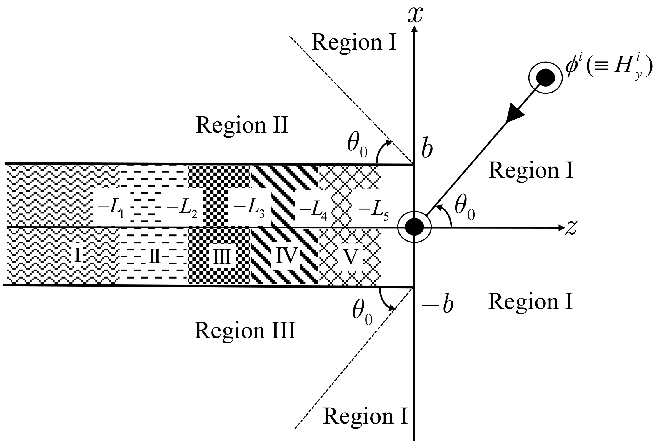
Diffraction by a Semi-Infinite Parallel-Plate Waveguide with Five-Layer Material Loading: The Case of H-Polarization

Department of Electrical, Electronic and Communication Engineering, Chuo University, Tokyo 112-8551, Japan
*
Author to whom correspondence should be addressed.
Appl. Sci. 2023, 13(6), 3715; https://doi.org/10.3390/app13063715
Submission received: 20 February 2023 / Revised: 10 March 2023 / Accepted: 13 March 2023 / Published: 14 March 2023

Abstract

:
In this paper, the plane wave diffraction from a semi-infinite parallel-plate waveguide with five-layer material loading is rigorously analyzed for H-polarization using the Wiener–Hopf technique. The Fourier transform of the scattered field is introduced and boundary conditions are applied in the transform domain to formulate the problem as simultaneous Wiener–Hopf equations, which are solved by the factorization and decomposition procedure leading to exact and approximate solutions. The scattered field in real space is explicitly derived by taking the Fourier inverse of the solution in the transform domain. For the region inside the waveguide, the scattered field is represented by the waveguide TM modes, and the field outside the waveguide is evaluated asymptotically by applying the saddle-point method to obtain a far-field expression. Numerical examples of the radar cross section (RCS) for various physical parameters are presented, and far-field scattering characteristics of the waveguide are discussed in detail.

1. Introduction

Accurate prediction and reduction of the radar cross section (RCS) is essential for the analysis of electromagnetic wave scattering from objects and radar absorbing materials (RAM) [1,2,3,4,5,6]. In recent years, there has been a lot of interest in multi-layer radar absorbers as a means of predicting and reducing the RCS of objects [7,8]. Meanwhile, simple geometric elements like plates, shells, spheres, and edges can be used to model complex objects like aircrafts or vehicles. In the past, scattering and diffraction properties of these simple geometric elements have been analyzed to understand how to predict or reduce the RCS of complex objects. One important geometry in this context is the open-ended metallic waveguide cavity [1,2,3,4,5,6,9], which is commonly encountered in various engineering applications, such as microwave filters, antennas, and transmission lines. In addition, it can be used as a base model for duct structures, such as jet engine intakes, and for the analysis of surface cracks on more complex objects. A variety of high-frequency and numerical methods, as well as hybrid ray-numerical methods [10,11,12,13,14,15,16,17,18,19,20,21,22], have been used to study the scattering from cavities of various shapes, but these methods may not provide uniformly valid solutions for any cavity size.
The Wiener–Hopf technique is known to be a powerful and rigorous method for the analysis of wave scattering and diffraction problems involving canonical geometries [23,24,25,26,27]. It has been successfully applied to a wide range of problems, including those involving semi-infinite media, planar interfaces, and layered media [26,27]. The technique is based on the use of the Wiener–Hopf equation, which arises from the requirement that the fields in two half-spaces satisfy certain boundary conditions. The solution of the Wiener–Hopf equation consists of decomposing the associated symbolic function into its positive and negative frequency components, which allows the problem to be reduced to a set of algebraic equations that can be solved to obtain the unknown field components. The advantage of the Wiener–Hopf technique is that it can handle problems involving arbitrary angles of incidence and polarization states, and it can also be used to study problems with multiple scattering or diffraction orders. In addition, the Wiener–Hopf technique has been applied to solve problems in various fields of physics and engineering, such as electromagnetism, acoustics, and seismology. It allows the determination of unknown fields and scattering coefficients by using complex variable analysis and contour integration. Although the method can be computationally intensive, it provides exact solutions for a wide range of problems and is highly valuable in the analysis of wave phenomena. Especially for the analysis of plane wave scattering by half-planes, parallel plate waveguides, and waveguide cavities, the Wiener–Hopf technique has been widely used to obtain strong solutions [28,29,30,31,32,33,34,35,36,37].
In the previous papers, the authors have performed a rigorous RCS analysis of various two-dimensional cavities formed by finite parallel-plate waveguides [38,39,40,41,42] and semi-infinite parallel-plate waveguides [43,44,45] using the Wiener–Hopf technique. Our final solutions have been proven to be effective over a wide range of frequencies and can be used to validate other commonly used numerical methods and high-frequency ray techniques. In our very recent paper [46], we have considered a semi-infinite parallel-plate waveguide with five-layer material loading that can form cavities and rigorously analyze the E-polarized plane wave diffraction using the Wiener–Hopf technique. It has been verified that our final solution is uniformly valid for arbitrary waveguide dimensions and any homogeneous material layers. In this paper, we will be examining the diffraction problem of the H-polarized plane wave incidence using the Wiener–Hopf technique, and we will be utilizing a waveguide geometry that is identical to the one presented in [36]. The geometry considered in this paper serves as an important generalization to our previous paper that analyzes a simpler case of four-layer material loading [47]. Due to the existence of five material layers in the waveguide, the analysis procedure becomes much more complicated compared to the four-layer case [47], as the multiple reflection-refraction-diffraction effect inside the waveguide is rigorously taken into account in this paper.
Applying the factorization and decomposition procedure, the Wiener–Hopf equations are solved exactly. The exact solution, however, is formal since it contains infinite series of terms with unknown coefficients. Employing the edge condition rigorously, we can find the asymptotic behavior of the unknowns leading to highly-accurate approximate solutions of the Wiener–Hopf equations. The results are shown to be uniformly valid for arbitrary waveguide dimensions. Taking the inverse Fourier transform of the solution in the transform domain and evaluating the resultant integrals, we can derive the scattered field representation real space. The scattered field inside the waveguide can be evaluated by computing the residue contributions from an infinite number of simple poles leading to the waveguide TM modes. The saddle point method is used to asymptotically estimate the scattering field outside the waveguide, yielding a far-field expression. Based on these analytical results, we will provide numerical examples of RCS for a range of physical parameters, along with a detailed analysis of the far-field scattering properties of the waveguide. We shall also make some comparisons with the E-polarized case [46].
Throughout this paper, we assume that the time factor is represented by e i ω t and is subsequently omitted for the sake of brevity and clarity.

2. Formulation of the Problem

We examine a semi-infinite parallel-plate waveguide that has a five-layer material loading and is excited by an H-polarized plane wave. The structure of the waveguide is depicted in Figure 1 and features infinitely thin plates that are uniformly conducting in the y-direction. The relative permittivity and permeability ( ε m , μ m ) for m = 1, 2, 3, 4, and 5 characterize the material layers I, II, III, IV, and V, respectively.
Let the total magnetic field ϕ t ( x , z ) [ H y t ( x , z ) ] be
ϕ t ( x , z ) = ϕ i ( x , z ) + ϕ ( x , z )
for < x < and < z < , where ϕ i ( x , z ) is the incident field of H-polarization defined by
ϕ i ( x , z ) = e i k ( x sin θ 0 + z cos θ 0 ) , 0 < θ 0 < π / 2
with k [ ω ( ε 0 μ 0 ) 1 / 2 ] being the free-space wavenumber. The total field ϕ t ( x , z ) satisfies the two-dimensional Helmholtz equation
[ 2 / x 2 + 2 / z 2 + μ ( x , z ) ε ( x , z ) k 2 ] ϕ t ( x , z ) = 0 ,
where
μ ( x , z ) = μ 1 ( layer   I ) μ 2 ( layer   II ) μ 3 ( layer   III ) μ 4 ( layer   IV ) μ 5 ( layer   V ) 1   ( otherwise ) , ε ( x , z ) = ε 1 ( layer   I ) ε 2 ( layer   II ) ε 3 ( layer   III ) ε 4 ( layer   IV ) ε 5 ( layer   V ) 1   ( otherwise ) ,
Once the solution of (3) is found, we derive non-zero components of the total electromagnetic field as follows:
( H y t , E x t , E z t ) = ϕ t , 1 i ω ε 0 ε x , z ϕ t z , i ω ε 0 ε x , z ϕ t x .
For the convenience of analysis, we assume that the vacuum is slightly lossy as in k = k 1 + i k 2 with 0 < k 2 k 1 . Taking the limit k 2 0 at the end of the analysis, we can obtain the solution for the lossless case. Taking into account the asymptotic behavior of the scattered field together with the radiation condition, we can show that
ϕ ( x , z ) = O ( e k 2 z cos θ 0 ) as   z , O ( e k 2 z )     as   z .
Let us define the Fourier transform of the scattered field with respect to z as
Φ ( x , α ) = ( 2 π ) 1 / 2 ϕ ( x , z ) e i α z d z ,
where α = σ + i τ ( Re α + i Im α ) . Using (6), we can show that Φ ( x , α ) is regular in the strip k 2 < τ < k 2 cos θ 0 of the complex α - plane . It can also be verified that as | x | , Φ ( x , α ) is bounded for any α in the strip k 2 < τ < k 2 cos θ 0 . We also introduce the Fourier integrals as
Φ + ( x , α ) = ( 2 π ) 1 / 2 0 ϕ ( x , z ) e i α z d z , Φ ( x , α ) = ( 2 π ) 1 / 2 L 1 ϕ t ( x , z ) e i α z d z , Φ m r ( x , α ) = ( 2 π ) 1 / 2 L m L m + 1 ϕ t ( x , z ) e i α z d z ,   m = 1 , 2 , 3 , 4 , Φ 1 0 ( x , α ) = ( 2 π ) 1 / 2 L 5 0 ϕ t ( x , z ) e i α z d z .
It follows from (6) that Φ + ( x , α ) and Φ ( x , α ) are regular in τ > k 2 and τ < k 2 cos θ 0 respectively, while Φ 1 0 ( x , α ) and Φ m r ( x , α ) for m = 1, 2, 3, 4 are all entire functions. In the following analysis, These conventions will be utilized to denote the areas of regularity in the complex α - plane . The use of (7) and (8), Φ ( x , α ) can be represented as:
Φ ( x , α ) = Φ 1 ( x , a ) + Ψ ( + ) ( x , α ) , < x < ,
where
Ψ ( + ) ( x , α ) = Φ + ( x , a ) A e i k x sin θ 0 α k cos θ 0 , A = 1 ( 2 π ) 1 / 2 i ,
Φ 1 ( x , α ) = m = 1 4 Φ m r ( x , α ) + Φ 1 0 ( x , α ) + Φ ( x , α ) .
As seen from (10), Ψ ( + ) ( x , α ) is regular in the upper half-plane τ > k 2 except for a simple pole α = k cos θ 0 . We shall henceforth use the subscript ‘(+)’ for functions with this property. We shall now derive the transformed wave equations by using the boundary conditions and the radiation condition.
According to (1) and (3), the scattered field ϕ ( x , z ) in the vacuum region satisfies
( 2 / x 2 + 2 / z 2 + k 2 ) ϕ ( x , z ) = 0 .
Furthermore, the total field ϕ t ( x , z ) satisfies
[ 2 / x 2 + 2 / z 2 + k r m 2 ] ϕ t ( x , z ) = 0
for m = 1, 2, 3, 4, and 5 for regions I, II, III, IV, and V, respectively, where k r m = ( μ r m ε r m ) 1 / 2 k . By taking the Fourier transform of (12) and applying (6) to the region | x | > b , it can be verified that
( d 2 / d x 2 γ 2 ) Φ ( x , α ) = 0
holds in the strip k 2 < τ < k 2 cos θ 0 , where
γ = ( α 2 k 2 ) 1 / 2 , Re γ > 0 .
The transformed wave equation for | x | > b is given by (14).
The derivation of the conversion wave equation for the region | x | < b is complicated by the presence of multiple dielectric discontinuities on the z = L m surfaces at m = 1, 2, 3, 4, and 5. We multiply both sides of (12) by ( 2 π ) 1 / 2 e i α z and integrate with respect to z over the range L 5 < z < .Then by considering (6) and the boundary condition for tangential electromagnetic fields at z = L 5 , we derive that
( d 2 / d x 2 γ 2 ) Φ 1 0 ( x , α ) + Ψ ( + ) ( x , α ) = e i α L 5 ε r 5 1 f 5 ( x ) i α g 5 ( x )
for τ > k 2 with α k cos θ 0 , where
f 5 ( x ) = ( 2 π ) 1 / 2 ϕ t ( x , L 5 0 ) z ,
g 5 ( x ) = ( 2 π ) 1 / 2 ϕ t ( x , L 5 0 ) .
Next, we multiply both sides of (13) by ( 2 π ) 1 / 2 e i α z and integrate with respect to z over the ranges < z < L 1 , L 1 < z < L 2 , L 2 < z < L 3 , L 3 < z < L 4 , and L 4 < z < L 5 . Using the boundary conditions for tangential electromagnetic fields at z = L m for m = 1, 2, 3, 4, and 5, we obtain
( d 2 / d x 2 Γ 1 2 ) Φ ( x , α ) = e i α L 1 f 1 ( x ) i α g 1 ( x ) ,
( d 2 / d x 2 Γ 2 2 ) Φ 1 r ( x , α ) = e i α L 2 f 2 ( x ) i α g 2 ( x ) + e i α L 1 ( ε r 2 / ε r 1 ) f 1 ( x ) i α g 1 ( x ) ,
( d 2 / d x 2 Γ 3 2 ) Φ 2 r ( x , α ) = e i α L 3 f 3 ( x ) i α g 3 ( x ) + e i α L 2 ( ε r 3 / ε r 2 ) f 2 ( x ) i α g 2 ( x ) ,
( d 2 / d x 2 Γ 4 2 ) Φ 3 r ( x , α ) = e i α L 4 f 4 ( x ) i α g 4 ( x ) + e i α L 3 ( ε r 4 / ε r 3 ) f 3 ( x ) i α g 3 ( x ) ,
( d 2 / d x 2 Γ 5 2 ) Φ 4 r ( x , α ) = e i α L 5 f 5 ( x ) i α g 5 ( x ) + e i α L 4 ( ε r 5 / ε r 4 ) f 4 ( x ) i α g 4 ( x )
where Γ m = ( α 2 k r m 2 ) 1 / 2 with Re Γ m > 0 for m = 1, 2, 3, 4, 5, and
f m ( x ) = ( 2 π ) 1 / 2 ϕ t ( x , L m 0 ) z m = 1 ,   2 ,   3 ,   4 ,   5 ,
g m ( x ) = ( 2 π ) 1 / 2 ϕ t ( x , L m ) m = 1 ,   2 ,   3 ,   4 ,   5 .
The transformed wave equations for x < b are represented by (16) and (19)–(23).
Considering the radiation condition, the solution to (14) can be written as:
Φ ( x , α ) = γ 1 Ψ ( + ) ( b , α ) e γ ( x b ) for   x > b , γ 1 Ψ ( + ) ( b , α ) e γ ( x + b )   for   x < b ,
with the prime denoting the x - derivative, the expression has been derived by utilizing (9) and applying the boundary conditions for tangential electromagnetic fields across x = ± b . Equation (26) denotes the representation of the scattered field for | x | > b .
Due to the medium discontinuities in | x | < b , the transformed wave equations contain unknown inhomogeneous terms f m ( x ) and g m ( x ) for m = 1, 2, 3, 4, 5. For convenience, we expand these functions into the Fourier cosine series as
f m ( x ) g m ( x ) = 1 b n = 1 n ν n f m n g m n cos n π 2 b ( x + b ) , ν n = 1 ,   n 1 ν 0 = 1 / 2
for | x | < b . Then, by following a procedure similar to that in our previous paper [46], we arrive at the solutions of (16) and (19)–(23), resulting in
Φ ( x , α ) = e i α L 1 b n = 1 ν n C 1 n ( α ) α 2 + Γ 1 n 2 cos n π 2 b ( x + b ) ,
Φ 1 0 ( x , α ) + Ψ ( + ) ( x , α ) = Ψ ( + ) ( b , α ) cosh γ ( x + b ) γ sinh 2 γ b Ψ ( + ) ( b , α ) cosh γ ( x b ) γ sinh 2 γ b 1 b n = 0 ν n C 5 n ( α ) α 2 + γ n 2 cos n π 2 b ( x + b )
Φ m r ( x , α ) = 1 b n = 0 ν n C m n ( α ) α 2 + Γ m n 2 cos n π 2 b ( x + b ) , m = 1 , 2 , 3 , 4 ,
where
γ 0 = i k , γ n = ( n π / 2 b ) 2 k 2 1 / 2 ,
  Γ m n = ( n π / 2 b ) 2 k r m 2 1 / 2 ,   m = 1 , 2 , 3 , 4 , 5 ,
C 5 n ( α ) = e i α L 5 C 5 n + ( α ) ,
C m n ( α ) = e i α L m + 1 C ( m + 1 ) n ( α ) e i α L m C m n + ( α ) for   m = 1 , 2 , 3 , 4
with
C m n ( α ) = f m n i α g m n , m = 1 , 2 , 3 , 4 , 5
C m n + ( α ) = ( ε r m + 1 / ε r m ) f m n i α g m n , m = 2 , 3 , 4 , 5
Here the Fourier coefficients f m n and g m n for m = 1, 2, 3, 4, 5 are defined by (A5) and (A6) in Appendix A. The representation of the scattered field for the region | x | < b is obtained by substituting (16) and (19)–(23) into (11) and utilizing (9).
Based on the above results, the desired scattered field representation in the Fourier transform domain is found to be
Φ ( x , α ) = γ 1 Ψ ( + ) ( ± b , α ) e γ ( x b ) for   x ± b ,     = Ψ ( + ) ( b , α ) cosh γ ( x + b ) γ sinh 2 γ b Ψ ( + ) ( b , α ) cosh γ ( x b ) γ sinh 2 γ b   1 b n = 0 ν n C 5 n ( α ) α 2 + γ n 2 cos n π 2 b ( x + b )   1 b n = 0 ν n C 1 n ( α ) α 2 + Γ 1 n 2 cos n π 2 b ( x + b )   1 b m = 1 4 n = 0 ν n C m n ( α ) α 2 + Γ m n 2 cos n π 2 b ( x + b ) for   x < b .
Equation (37) holds in the strip k 2 < τ < k 2 cos θ 0 of the complex α - plane.
Differentiating (37) with respect to x , setting x = ± b ± 0 ,   ± b 0 in the results, after manipulating the equations with the help of the boundary conditions, we can deduce that
J d ( α ) = U ( + ) ( α ) M ( α ) 2 b n = 1 , odd e i α L 5 C 5 n + α α 2 + γ n 2   + 2 b n = 1 , odd e i α L 1 C 1 n + α α 2 + Γ 1 n 2   + 2 b m = 2 5 n = 1 , odd e i α L m C m n α e i α L m 1 C ( m 1 ) n + α α 2 + Γ m n 2 ,
J s ( α ) = V ( + ) ( α ) N ( α ) + 2 b n = 0 , even ν n e i α L 5 C 5 n + α α 2 + γ n 2   2 b n = 0 , even ν n e i α L 1 C 1 n + α α 2 + Γ 1 n 2   2 b m = 2 5 n = 0 , even ν n e i α L m C m n α e i α L m 1 C ( m 1 ) n + α α 2 + Γ m n 2 ,
where
U ( + ) ( α ) = Ψ ( + ) ( b , α ) + Ψ ( + ) ( b , α ) ,
V ( + ) ( α ) = Ψ ( + ) ( b , α ) Ψ ( + ) ( b , α ) ,
J d ( α ) = J ( b , α ) J ( b , α ) ,
J s ( α ) = J ( b , α ) + J ( b , α ) ,
M ( α ) = γ e γ b cosh γ b ,   N ( α ) = γ e γ b sinh γ b ,
J ( ± b , α ) = Φ ( ± b ± 0 , α ) Φ 1 ( ± b 0 , α ) .
The unknown spectral functions fulfill the Wiener–Hopf equations expressed in Equations (38) and (39).

3. Exact and Approximate Solutions

The kernel functions M ( α ) and N ( α ) given by (44) are factorized as [23,24]
M ( α ) = M + ( α ) M ( α ) = M + ( α ) M + ( α ) , N ( α ) = N + ( α ) N ( α ) = N + ( α ) N + ( α ) ,
where
M + ( α ) = cos k b 1 / 2 e i 3 π / 4 k + α 1 / 2 exp i γ b π ln α γ k exp i α b π 1 C + ln π 2 k b + i π 2 n = 1 , odd 1 + α i γ n   e 2 i α b / n π ,
N + ( α ) = k sin k b 1 / 2 e i π / 2 exp i γ b π ln α γ k exp i α b π π 1 C + ln π 2 k b + i π 2 1 + α i γ 0 n = 2 , even 1 + α i γ n   e 2 i α b / n π .
with C (= 0.57721566 …) being Euler’s constant. According to (46)–(48), M ± ( α ) and N ± ( α ) are regular and nonzero in τ k 2 , and show the following asymptotic behavior:
M ± ( α ) , N ± ( α ) ( i α / 2 ) 1 / 2       as α   with   τ k 2 .
We multiply both sides of (38) by M ( α ) and decompose the resultant equations. This leads to
M ( α ) J d ( α ) 2 π 1 / 2 i cos ( k b sin θ 0 ) M + ( k cos θ 0 ) ( α k cos θ 0 ) + n = 1 , odd n π b 2 1 α + i γ n M ( α ) e i α L 5 C 5 n + ( α ) α i γ n + M + ( i γ n ) e γ n L 5 C 5 n + ( i γ n ) 2 i γ n + n = 1 , odd n π b 2 1 α + i γ n M ( α ) e i α L 1 C 1 n ( α ) α i Γ 1 n + M + ( i Γ 1 n ) e Γ 1 n L 1 C 1 n + ( i Γ 1 n ) 2 i Γ 1 n + m = 2 5 1 α + i Γ m n M ( α ) e i α L m C m n ( α ) e i α L m 1 C ( m 1 ) n + ( α ) α i Γ m n + M + ( i Γ m n ) e i α L m C m n ( i Γ m n ) e i α L m 1 C ( m 1 ) n + ( i Γ m n ) 2 i Γ m n = U ( + ) ( α ) M + ( α ) + 2 π 1 / 2 i cos ( k b sin θ 0 ) M + ( k cos θ 0 ) ( α k cos θ 0 ) + n = 1 , odd n π b 2 M + ( i γ n ) e γ n L 5 C 5 n + ( i γ n ) 2 i γ n ( α + i γ n ) n = 1 , odd n π b 2 M + ( i Γ 1 n ) e Γ 1 n L 1 C 1 n + ( i Γ 1 n ) 2 i Γ 1 n ( α + i Γ 1 n ) m = 2 , odd 5 n π b 2 M + ( i Γ m n ) e Γ m n L m C m n ( i Γ m n ) e Γ m n L m 1 C ( m 1 ) n + ( i Γ m n ) 2 i Γ m n ( α + i Γ m n ) .
Based on Meixner’s edge conditions [24,48], we deduce that
ϕ ( ± b , z ) x = i k sin θ 0 e i k ( ± b sin θ 0 + z cos θ 0 ) + O ( z 1 / 2 ) ,   for   L 5 > 0 ,   as   z + 0 , i k sin θ 0 e i k ( ± b sin θ 0 + z cos θ 0 ) + O ( z 1 + ν ) ,   for   L 5 = 0 ,   as   z + 0 ,
ϕ t ( ± b ± 0 , z ) ϕ t ( ± b 0 , z ) = O ( z 1 / 2 ) ,   for   L 5 > 0 ,   as   z 0 , O ( z ν ) ,   for   L 5 = 0 ,   as   z 0 ,
where
ν = η ( ν μ + 1 , ν ε )
with Re ν > 0 , Re ν > 0 , and
ν μ = 1 π cos 1 μ γ 1 2 ( μ γ + 1 ) , ν ε = 1 π cos 1 1 ε r 2 ( 1 + ε r ) ,
η ( a , b ) = a   for   Re a Re b , b   for   Re a Re b .
Applying the fundamental theorem for the asymptotic behaviors of the Fourier integrals [25], we can show that Ψ ( + ) ( ± b , α ) and J ( ± b , α ) asymptotically behave like
Ψ ( + ) ( ± b , α ) = O ( α 1 / 2 ) , for   τ > k 2 ,   for   L 5 > 0 ,         = O ( α ν ) , for   τ > k 2 ,   for   L 5 = 0 ,
J ± b , α = O α 3 / 2 ,   for   τ < k 2 cos θ 0 ,   for   L 5 > 0 ,           = O α 1 ν ,   for   τ < k 2 cos θ 0 ,   for   L 5 = 0 .
as α . Thus, applying (56) and (57) to (40) and (42), respectively, we can obtain
U ( + ) ( α ) , V ( + ) ( α ) = O ( α 1 / 2 ) , for   τ > k 2 ,   for   L 5 > 0 ,   = O ( α ν ) , for   τ > k 2 ,   for   L 5 = 0 ,
J s , d ( ± b , α ) = O ( α 3 / 2 ) , for   τ < k 2 cos θ 0 ,   for   L 5 > 0 ,   = O ( α 1 ν ) , for   τ < k 2 cos θ 0 ,   for   L 5 = 0 .
It is shown that the left- and right-hand sides of (50) are regular in the lower ( τ < k 2 cos θ 0 ) and upper ( τ > k 2 ) half-planes, respectively, and both sides have a common strip of regularity ( k 2 < τ < k 2 cos θ 0 ) . By using the analytic continuation argument demonstrates, it can be shown that both sides of equation (50) must be equivalent to an entire function. Further, this function is determined to be identically zero by utilizing (58), (59), and Liouville’s theorem. Thus, it can be concluded that
U ( + ) ( α ) M + ( α ) 2 i k sin θ 0 cos ( k b sin θ 0 ) M + ( k cos θ 0 ) ( α k cos θ 0 ) + n = 1 , odd M + ( i γ n ) e γ n L 5 C 5 n + ( i γ n ) 2 i γ n ( α + i γ n ) = 0 .
The same procedure can be employed to solve a different Wiener–Hopf Equation (39). Omitting the particulars, we arrive at
V ( + ) ( α ) N + ( α ) + 2 k sin θ 0 sin ( k b sin θ 0 ) N + ( k cos θ 0 ) ( α k cos θ 0 ) n = 0 , even ν n N + ( i γ n ) e γ n L 5 C 5 n + ( i γ n ) 2 i γ n ( α + i γ n ) = 0 .
Equations (60) and (61) involve the unknown coefficients C 5 n + i γ n . Appendix A contains an analysis of the correlation between the unknown functions and the unknown Fourier coefficients. Using (A21) in (60) and (61) and rearranging the results, we are led to
U ( + ) ( α ) b = M + ( α ) b 1 / 2 A u b α k cos θ 0 n = 1 δ 2 n 1 a n p n u n + b α + i γ 2 n 1 ,
V ( + ) ( α ) b = N + ( α ) b 1 / 2 A v b α k cos θ 0 n = 1 ν 2 n 2 δ 2 n 2 b n q n v n + b α + i γ 2 n 2 ,
where
A u = 2 b π 1 / 2 k sin θ 0 cos ( k b sin θ 0 ) M + ( k cos θ 0 ) , A v = 2 b π 1 / 2 i k sin θ 0 sin ( k b sin θ 0 ) N + ( k cos θ 0 ) ,
a n = b i γ 2 n 1 1 ,   n 0 , b n = b i γ 2 n 2 1 ,   n 1 ,  
p n = b 1 / 2 M + ( i γ 2 n 1 ) ,   n 0 , q n = b 1 / 2 N + ( i γ 2 n 2 ) ,   n 1 ,
u n + = U ( + ) ( i γ 2 n 1 ) , v n + = V ( + ) ( i γ 2 n 2 ) ,   n 0 .
Equations (62) and (63) provide the exact solutions to the Wiener–Hopf Equations (38) and (39), respectively. However, they remain formal as they entail infinite series with unknown coefficients u n + and v n + for n = 1 ,   2 ,   3 , are involved. Using (58) and (67), we find that
u n + 2 1 / 2 K u ( b γ 2 n 1 ) 1 / 2 , v n + 2 1 / 2 K v ( b γ 2 n 2 ) 1 / 2 ,   for   L 5 > 0 , u n + 2 1 / 2 K u ( b γ 2 n 1 ) ν , v n + 2 1 / 2 K v ( b γ 2 n 2 ) ν ,   for   L 5 = 0
as n , where K u and K v are unknown constants. By choosing a large positive integer N, the unknowns u n + and v n + for n N in the infinite series of (62) and (63) can be approximated with reasonable accuracy by the asymptotic behavior given in (68). This consideration shows that it is feasible to substitute each infinite series present in (62) and (63) with the sum of a finite series containing N-1 unknowns and the remaining infinite series with a single unknown constant. Thus we obtain approximate expressions of (62) and (63) as in
U ( + ) ( α ) b M + ( α ) b 1 / 2 A u b α k cos θ 0 n = 1 N 1 δ 2 n 1 a n p n u n + b α + i γ 2 n 1 + K u S u ( α ) ,
V ( + ) ( α ) b N + ( α ) b 1 / 2 A v b α k cos θ 0 n = 1 δ 2 n 2 b n q n v n + b α + i γ 2 n 2 + K v S v ( α ) ,
where
S u N ( α ) = n = N δ 2 n 1 ( b γ 2 n 1 ) 1 b α + i γ 2 n 1 ,   S v N ( α ) = n = N δ 2 n 2 ( b γ 2 n 2 ) 1 b α + i γ 2 n ,   for   L 5 > 0 , S u N ( α ) = n = N δ 2 n 1 ( b γ 2 n 1 ) 1 / 2 ν b α + i γ 2 n 1 ,   S v N ( α ) = n = N δ 2 n 2 ( b γ 2 n 2 ) 1 / 2 ν b α + i γ 2 n ,   for   L 5 = 0 .
Equations (69) and (70) provide approximate expressions of (62) and (63), respectively, where the unknowns u n + and v n + for n = 1 ,   2 ,   3 ,   ,   N 1 ,   K u and K v are also included. These unknowns can be determined numerically by solving the two sets of N × N matrix equations. It is important to note that (69) and (70) have been derived on the basis of the edge condition and hence, are valid for arbitrary waveguide dimension.

4. Scattered Field

The scattered field in real space can be obtained by performing the inverse Fourier transform using the following formula:
ϕ ( x , z ) = ( 2 π ) 1 / 2 + i c + i c Φ ( x , α ) e i α z d α ,     k 2 < c < k 2 cos θ 0 .
By substituting (37) into (72) and evaluating the resulting integral, we can explicitly derive the scattered field in real space. The scattered field inside the waveguide can be derived by computing the residues at an infinite number of simple poles. This yields,
ϕ ( x , z ) = ϕ i ( x , z ) + n = 0 T 1 n e Γ 1 n ( z + L 1 ) cos n π 2 b ( x + b ) for < z < L 1 , ( region I ) ,       = ϕ i ( x , z ) + n = 0 T m n e Γ m n z + L m T m n + e Γ m n z + L ( m 1 ) cos n π 2 b ( x + b ) ,       ( m = 2 , 3 , 4 , 5 ) for L 1 < z < L 5 , ( region II , III , IV , V ) ,       = ϕ i ( x , z ) + n = 1 T 0 e γ n ( z + L 5 ) T 0 + e γ n ( z + L 5 ) cos n π 2 b ( x + b ) for L 5 < z < 0 ,
where
T m n = π 2 1 / 2 P m n b Γ m n e γ n L 5 U ( + ) i γ n , for   odd   n ,   ( m = 1 , 2 , 3 , 4 , 5 , ) ,     = π 2 1 / 2 ν n P m n b Γ m n e γ n L 5 V ( + ) i γ n , for   even   n , ( m = 1 , 2 , 3 , 4 , 5 , ) .  
T m n + = π 2 1 / 2 Q m n b Γ ( m + 1 ) n e γ n L 5 U ( + ) i γ n , for   odd   n , ( m = 1 , 2 , 3 , 4 ) , = π 2 1 / 2 ν n Q m n b Γ ( m + 1 ) n e γ n L 5 V ( + ) i γ n , for   even   n , ( m = 1 , 2 , 3 , 4 ) .
T 0 = π 2 1 / 2 e γ n L 5 b γ n U ( + ) i γ n , for   odd   n , = π 2 1 / 2 n π 2 b 2 e γ n L 5 γ n V ( + ) i γ n , for   even   n .
T 0 + = π 2 1 / 2 Q 5 n b γ n e γ n L 5 U ( + ) i γ n , for   odd   n ,     = π 2 1 / 2 ν n Q 5 n b γ n e γ n L 5 V ( + ) i γ n , for   even   n .
In (73)–(77), P m n and Q m n for m = 1, 2, 3, 4, 5 are defined in Appendix A.
We now take into account the region outside the waveguide and derive the scattered far field. The region outside the waveguide includes x < b with z > 0 , as well as x > b . However, at large distances from the origin, the contributions from x < b outside the waveguide are negligibly small and hence, we will not consider this region. By using (37) and (72), an integral representation for the scattered field for x > b is found to be
ϕ ( x , z ) = ( 2 π ) 1 / 2 + i c + i c Ψ ( + ) ± b , α e γ ( x b ) i α z d α ,
where Ψ ( + ) ± b , α can be expressed as follows:
Ψ ( + ) ( ± b , α ) = 1 2 U ( + ) ( α ) ± V ( + ) ( α ) .
Employing a procedure similar to that utilized in [46], we arrive at (80)
ϕ ( ρ 1 , 2 , θ 1 , 2 ) Ψ ( + ) ± b , k cos θ 1 , 2 Φ ˜ ± b , k cos θ 1 , 2 k sin θ 1 , 2 e i k ρ 1 , 2 3 π / 4 k ρ 1 , 2 1 / 2 e i k b sin θ 0 e i k ρ 1 , 2 cos θ 1 , 2 θ 0 F 2 k ρ 1 , 2 1 / 2 cos θ 1 , 2 θ 0 / 2 + e i k ρ 1 , 2 cos θ 1 , 2 + θ 0 F 2 k ρ 1 , 2 1 / 2 cos θ 1 , 2 + θ 0 / 2 , x ± b ,
where ( ρ 1 , 2 , θ 1 , 2 ) are the cylindrical coordinates given by
x b = ρ 1 sin θ 1 , z = ρ 1 cos θ 1 for   0 < θ 1 < π , x + b = ρ 2 sin θ 2 , z = ρ 2 cos θ 2 for   π < θ 2 < 0 ,
and F is the Fresnel integral defined by
F ω = e i π / 4 π 1 / 2 ω e i t 2 d t .
Equation (80) gives an asymptotic expression of the scattered field as k ρ 1 , 2 , which is uniformly valid in observation angles θ 1 , 2 .
Introducing the cylindrical coordinate ρ , θ as x = ρ sin θ ,   z = ρ cos θ for π < θ < π , It is evident that the following approximate relationship holds in the far field.
cos θ 1 cos θ cos θ 2 ,
ρ 1 ρ b sin θ , for   0 < θ < π ,
ρ 2 ρ + b sin θ , for   π < θ < 0 .
By substituting an asymptotic expansion of the Fresnel integral in (80) with large k ρ 1 , 2 and using (83)–(85), we can obtain an alternative form for the scattered far field
ϕ ρ , θ ϕ g ρ , θ + ϕ d ρ , θ , θ 1 , 2 π θ 0 .
where ϕ g ρ , θ and ϕ d ρ , θ are the geometrical optics field and the diffraction field, respectively, and are defined by
ϕ g ρ , θ = e i k ρ cos ( θ θ 0 ) ,   for   π < θ 2 < π + θ 0 , 0 ,   for   π + θ 0 < θ 2 < 0 ,   0 < θ 1 < π θ 0 , e 2 i k b sin θ 0 e i k ρ cos ( θ + θ 0 ) ,   for   π θ 0 < θ 1 < π .
ϕ d ρ , θ = Ψ ( + ) ± b , k cos θ k sin θ e i k b sin θ e i k ρ 3 π / 4 k ρ 1 / 2 ,   for   θ 0 .

5. Numerical Results and Discussion

This section focuses on illustrative numerical examples of RCS, which we use to study in detail the far-field backscattering properties of waveguides. We define the RCS per unit length as follows
σ = lim ρ 2 π ρ ϕ d 2 ϕ i 2 ,
where ϕ d is the diffracted field defined by (88). For real k , (89) is simplified by using (2), (79), and (88) as
σ = λ 2 U ( + ) ( k cos θ ) ± V ( + ) ( k cos θ ) 2
for θ 0 with λ being the free-space wavelength. By using the approximate expressions in (62) and (63), we have calculated U ( + ) ( k cos θ ) and V ( + ) ( k cos θ ) involved in (90). We need to numerically invert the two sets of N × N matrix equations to obtain physical quantities. We have verified by careful numerical experiments that the choice N 2 k b / π in (62) and (63) generates sufficiently accurate results.
Figure 2, Figure 3, Figure 4 and Figure 5 show the normalized monostatic RCS σ / λ versus incidence angle θ 0 , where the value of σ / λ is plotted in decibels [dB] by calculating 10 log 10 σ / λ . Figure 6 shows the monostatic RCS [dB] versus normalized frequency kb. Figure 7 and Figure 8 show comparisons of the angular and frequency characteristics of the monostatic RCS, respectively, between E-polarization [46] and H-polarization (this paper). In order to investigate the scattering mechanism over a wide frequency range, six typical values of the normalized waveguide aperture width have been chosen as kb = 1.57, 3.14, 15.7, 31.4, 47.1, and 62.8. In addition, the ratio   L 1 / 2 b has been chosen as 0.5 (Figure 2), 1.0 (Figure 3), 3.0 (Figure 4), and 5.0 (Figure 5). For numerical computations, we have selected five different materials from the RAM study by Michielssen et al. [6]. It is important to note here that although these material properties are fictitious, they represent a wide range of available radar absorbing materials. The material constants are ε 1 = 8 + i 10 ,   μ 1 = 1 + i 0 for region I, ε 2 = 10 + i 6 ,   μ 2 = 1 + i 0 for region II, ε 3 = 15 + i 0 ,     μ 3 = 3 + i 15 for region III, ε 4 = 15 + i 0 ,   μ 4 = 7 + i 12 for region IV, and ε 5 = 15 + i 0 ,     μ 5 = 25.8 + i 10.3 for region V. The thickness of the material in region I extends from L 5 to . The thickness of regions II, III, IV, and V is such that L 1 L 2 = L 2 L 3 = L 3 L 4 = L 4 L 5 = t / 4 , and the total thickness of the four-layer material (regions II–V) is taken as k t = 1.57 . Figure 2, Figure 3, Figure 4, Figure 5 and Figure 6 include the results from one- to four-layer material loading for comparison.
From Figure 2, Figure 3, Figure 4 and Figure 5 for angular dependences, it is observed that the RCS exhibits large values over a certain range of the incidence angle due to the internal irradiation and reduces with an increase of the number of material layers. From these characteristics, we see that multi-layer loading gives rise to better RCS reduction over a wide range of frequencies. Another common feature in all numerical examples is that the RCS oscillates rapidly for larger kb and L 1 / 2 b . Comparing the characteristics for one- to five-layer cases in all numerical examples, better RCS reduction is observed in the five-layer case for all kb.
Next, we will examine the frequency dependences of the RCS to gain a more comprehensive understanding of the backscattering characteristics. Figure 6 presents the normalized monostatic RCS as a function of the normalized frequency kb, for angles of incidence θ 0 = 0 ° , 30 ° , and 60 ° with L 1 / 2 b = 1.0 . We have again considered five different geometries: waveguides with one-, two-, three-, four-, and five-layer material loading. The material properties and the material layer thicknesses are the same as in Figure 2. As shown in Figure 6a,b, the RCS level for single-layer loading increases almost monotonically with an increase of kb, while for multi-layer loading, the RCS is reduced with an increase in the number of layers over the entire frequency range. As for Figure 6c with θ 0 = 60 ° , the RCS value does not reduce even with an increase of the number of material layers and shows complicated features over the entire frequency range. This is because, for larger incidence angles, multiple reflections occur inside the waveguide leading to resonance phenomena.
Finally, let us discuss differences in the backscattering characteristics between H- and E-polarizations. From the angular dependences in Figure 7a for k b = 3.14 (low frequencies), the backscatter characteristics of the two polarizations are completely different from each other. It is also seen that H-polarization shows better RCS reduction characteristics than E-polarization at low frequencies. On the other hand, we observe from Figure 7b for k b = 62.8 (high frequencies) that the RCS characteristics for both polarizations become close to each other. Figure 8 shows a comparison of the frequency dependences between the two polarizations. It is interesting to note that there are great differences in the RCS characteristics, and in particular, the RCS oscillates more rapidly in the E-polarization than in H-polarization. This clearly shows that the resonance effect in the waveguide is stronger in the E-polarization.

6. Conclusions

In this paper, we have utilized the Wiener–Hopf technique to rigorously solve the diffraction of H-polarized plane waves by a semi-infinite parallel-plate waveguide loaded with a five-layer material. Our final solution is valid for waveguides of arbitrary dimensions and can serve as a benchmark for validating more general solution methods. Through the use of numerical examples, we have explored the monostatic radar cross section (RCS) for various physical parameters, delving into the waveguide’s far-field backscattering properties in detail. Our analysis highlights the crucial role played by multi-layer material loading in RCS reduction over a wide frequency range. Additionally, we have compared our results for H-polarization with those obtained for E-polarization in [36], and elucidated the differences that arise based on the incident polarizations.

Author Contributions

Methodology, K.H. and K.K.; Validation, K.H.; Formal analysis, K.H. and K.K.; Investigation, K.H.; Resources, K.H.; Data curation, K.H.; Writing–original draft, K.H.; Writing–review & editing, K.H. and K.K.; Supervision, K.K. All authors have read and agreed to the published version of the manuscript.

Funding

This research received no external funding.

Institutional Review Board Statement

Not applicable.

Informed Consent Statement

Not applicable.

Data Availability Statement

Not applicable.

Conflicts of Interest

The authors declare no conflict of interest.

Appendix A. Some Properties of the Fourier Coefficients

In this Appendix A, we study analytical properties of the Fourier coefficients f m n and g m n for m = 1 , 2 , 3 , 4 , 5 that appear in (27). Based on the definition, Ψ ( + ) ( x , α ) is regular in τ > k 2 except for a simple pole at α = k cos θ 0 , whereas Φ ( x , α ) is regular in τ < k 2 cos θ 0 . In addition, Φ m r ( x , α ) with m = 2 ,   3 ,   4 ,   5 , and Φ 1 0 ( x , α ) are all entire functions. Therefore, it follows that
lim α i γ n ( α i γ n ) Φ 1 0 ( x , α ) + Ψ ( + ) ( x , α ) = 0 ,
lim α ± i Γ m n ( α i Γ m n ) Φ m 1 r ( x , α ) = 0 , m = 2 , 3 , 4 , 5 .
Substituting (29) and (30) into (A1), (A2), respectively and carrying out some manipulations, we obtain that
C 5 n + ( i γ n ) = n π 2 b U ( + ) ( i γ n )   for   odd   n ,   = n π 2 b V ( + ) ( i γ n ) for   even   n ,
and
C m n ( ± i Γ m n ) = 0 , n = 1 , 2 , 3 , .
with m =   2 ,   3 ,   4 ,   5 , Equations (38) and (39) define the unknown functions U + α and V + α . The set of Equations (A3) and (A4) provide a system of simultaneous algebraic equations that establish a connection between the unknown functions U ( + ) ( α ) and U ( + ) ( α ) and the Fourier coefficients f n m and g m n , for m = 1, 2, 3, 4, 5. By solving these equations for f n m and g m n , we derive that
f m n = n π b P m n U ( + ) ( i γ n ) for   odd   n ,   = n π b P m n V ( + ) ( i γ n ) for   even   n .
g m n = n π b Q m n U ( + ) ( i γ n ) for   odd   n ,   = n π b Q m n V ( + ) ( i γ n ) for   even   n .
where
P 1 n = 2 Γ 1 n e Γ 2 n ( L 1 L 2 ) ( ε r 2 / ε r 1 ) Γ 1 n + Γ 2 n ( 1 + δ 1 n ) Γ 2 n e Γ 3 n ( L 2 L 3 ) ( ε r 3 / ε r 2 ) δ 1 n Γ 2 n + Γ 3 n · ( 1 + δ 2 n ) Γ 3 n e Γ 4 n ( L 3 L 4 ) ( ε r 4 / ε r 3 ) δ 2 n Γ 3 n + Γ 4 n ( 1 + δ 3 n ) ε r 5 Γ 4 n ( ε r 5 / ε r 4 ) δ 3 n Γ 4 n + Γ 5 n · 2 e Γ 5 n ( L 4 L 5 ) 1 ρ 4 n ρ 5 n e 2 Γ 5 n ( L 4 L 5 ) ε r 5 Γ 5 n ε r 5 γ n + Γ 5 n , .
P 2 n = ( 1 + δ 1 n ) Γ 2 n e Γ 3 n ( L 2 L 3 ) ( ε r 3 / ε r 2 ) δ 1 n Γ 2 n + Γ 3 n ( 1 + δ 2 n ) Γ 3 n e Γ 4 n ( L 3 L 4 ) ( ε r 4 / ε r 3 ) δ 2 n Γ 3 n + Γ 4 n       ( 1 + δ 3 n ) ε r 5 Γ 4 n ( ε r 5 / ε r 4 ) Γ 4 n + δ 3 n Γ 5 n ( 1 ρ 5 n ) e Γ 5 n ( L 4 L 5 ) 1 ρ 4 n ρ 5 n e 2 Γ 5 n ( L 4 L 5 ) ,
P 3 n = ( 1 + δ 2 n ) Γ 3 n e Γ 4 n ( L 3 L 4 ) ( ε r 4 / ε r 3 ) Γ 3 n + δ 2 n Γ 4 n ( 1 + δ 3 n ) ε r 5 Γ 4 n ( ε r 5 / ε r 4 ) δ 3 n Γ 4 n + Γ 5 n ( 1 ρ 5 n ) e Γ 5 n ( L 4 L 5 ) 1 ρ 4 n ρ 5 n e 2 Γ 5 n ( L 4 L 5 ) ,
P 4 n = ( 1 + δ 3 n ) ε r 5 Γ 4 n ( ε r 5 / ε r 4 ) δ 3 n Γ 4 n + Γ 5 n ( 1 ρ 5 n ) e Γ 5 n ( L 4 L 5 ) 1 ρ 4 n ρ 5 n e 2 Γ 5 n ( L 4 L 5 ) ,
P 5 n = 2 1 ρ 4 n ρ 5 n e 2 Γ 5 n ( L 4 L 5 ) ε r 5 Γ 5 n ε r 5 γ n + Γ 5 n ,
Q 1 n = ρ 1 n e Γ 2 n ( L 1 L 2 ) ( 1 + δ 1 n ) Γ 2 n e Γ 3 n ( L 2 L 3 ) ( ε r 3 / ε r 2 ) δ 1 n Γ 2 n + Γ 3 n ( 1 + δ 2 n ) Γ 3 n e Γ 4 n ( L 3 L 4 ) ( ε r 4 / ε r 3 ) δ 2 n Γ 3 n + Γ 4 n ( 1 + δ 3 n ) ε r 5 Γ 4 n ( ε r 5 / ε r 4 ) δ 3 n Γ 4 n + Γ 5 n 2 e Γ 5 n ( L 4 L 5 ) 1 ρ 4 n ρ 5 n e 2 Γ 5 n ( L 4 L 5 ) ε r 5 Γ 5 n ε r 5 γ n + Γ 5 n ,
Q 2 n = ρ 2 n e Γ 3 n ( L 2 L 3 ) ( 1 + δ 2 n ) Γ 3 n e Γ 4 n ( L 3 L 4 ) ( ε r 4 / ε r 3 ) Γ 3 n + δ 2 n Γ 4 n ( 1 + δ 3 n ) ε r 5 Γ 4 n ( ε r 5 / ε r 4 ) δ 3 n Γ 4 n + Γ 5 n ( 1 ρ 5 n ) e Γ 5 n ( L 4 L 5 ) 1 ρ 4 n ρ 5 n e 2 Γ 5 n ( L 4 L 5 ) ,
Q 3 n = ρ 3 n e Γ 4 n ( L 3 L 4 ) ( 1 + δ 3 n ) μ r 5 Γ 4 n ( ε r 5 / ε r 4 ) Γ 4 n + δ 3 n Γ 5 n 2 e 2 Γ 5 n ( L 4 L 5 ) 1 ρ 4 n ρ 5 n e 2 Γ 5 n ( L 4 L 5 ) ε r 5 Γ 5 n ε r 5 γ n + Γ 5 n ,
Q 4 n = ε r 5 ρ 4 n ( 1 ρ 5 n ) e Γ 5 n ( L 4 L 5 ) 1 ρ 4 n ρ 5 n e 2 Γ 5 n ( L 4 L 5 ) ,
Q 5 n = ρ 4 n e 2 Γ 5 n ( L 4 L 5 ) ρ 5 n 1 ρ 4 n ρ 5 n e 2 Γ 5 n ( L 4 L 5 )
with
ρ 1 n = ( ε r 2 / ε r 1 ) Γ 1 n Γ 2 n ( ε r 2 / ε r 1 ) Γ 1 n + Γ 2 n ,
ρ m n = ε r m + 1 / ε r 1 δ m 1 n Γ m n Γ m + 1 n ε r m + 1 / ε r 1 δ m 1 n Γ m n + Γ m + 1 n , m = 2 , 3 , 4 ,
ρ 5 n = ε r 5 γ n Γ 5 n ε r 5 γ n + Γ 5 n .
δ m n = 1 + ρ m n e 2 Γ m + 1 n L m L m + 1 1 ρ m n e 2 Γ m + 1 n L m L m + 1 , m = 1 , 2 , 3 .
By substituting (A5) and (A6) with m = 5 into (34) and setting α = i γ n , we also obtain
C 5 n ( i γ n ) = n π 2 b δ n U ( + ) ( i γ n ) for odd n ,           = n π 2 b δ n V ( + ) ( i γ n ) for even n ,
where
δ n = ρ 4 n e 2 Γ 5 n ( L 4 L 5 ) ρ 5 n e 2 γ n L 5 1 ρ 4 n ρ 5 n e 2 Γ 5 n ( L 4 L 5 ) .
Equations (A3)–(A6) and (A21) can be conveniently used to decompose the Wiener–Hopf Equations (38) and (39).

References

  1. Knott, E.F.; Shaeffer, J.; Tuley, M. Radar Cross Section, 2nd ed.; SciTech: Raleigh, NC, USA, 2004; pp. 269–367. [Google Scholar]
  2. Balanis, C.A. Advanced Engineering Electromagnetics, 2nd ed.; Wiley: New York, NY, USA, 2012; pp. 351–543. [Google Scholar]
  3. Stone, W.R. (Ed.) Radar Cross Sections of Complex Objects; IEEE Press: New York, NY, USA, 1990. [Google Scholar]
  4. Bhattacharyya, A.K.; Sengupta, D.L. Radar Cross Section Analysis and Control; Artech House: Boston, MA, USA, 1991. [Google Scholar]
  5. Bernard, J.M.L.; Pelosi, G.; Ufimtsev, P.Y. Special issue on radar cross section of complex objects. Ann. Telecommun. 1995, 50, 471–598. [Google Scholar]
  6. Michielssen, E.; Sajer, J.M.; Ranjithan, S.; Mittra, R. Design of lightweight, broad-band microwave absorbers using genetic algorithms. IEEE Trans. Microw. Theory Tech. 1993, 41, 1024–1031. [Google Scholar] [CrossRef]
  7. Zhou, D.; Huang, X.; Du, Z. Analysis and design of multilayered broadband radar absorbing metamaterial using the 3-D printing technology-based method. IEEE Antennas Wirel. Propag. Lett. 2017, 16, 133–136. [Google Scholar] [CrossRef]
  8. Toktas, A.; Ustun, D.; Tekbas, M. Multi-objective design of multilayer radar absorber using surrogate-based optimization. IEEE Trans. Microw. Theory Tech. 2019, 67, 3318–3329. [Google Scholar] [CrossRef]
  9. Pathak, P.H.; Bukholder, R.J. Electromagnetic Radiation, Scattering, and Diffraction; Wiley: New York, NY, USA, 2021; pp. 314–451. [Google Scholar]
  10. Lee, C.S.; Lee, S.-W. RCS of a coated circular waveguide terminated by a perfect conductor. IEEE Trans. Antennas Propag. 1987, 35, 391–398. [Google Scholar]
  11. Altintaș, A.; Pathak, P.H.; Liang, M.C. A selective modal scheme for the analysis of EM coupling into or radiation from large open-ended waveguides. IEEE Trans. Antennas Propag. 1988, 36, 84–96. [Google Scholar] [CrossRef]
  12. Ling, H.; Chou, R.-C.; Lee, S.-W. Shooting and bouncing rays: Calculating the RCS of an arbitrary shaped cavity. IEEE Trans. Antennas Propag. 1989, 37, 194–205. [Google Scholar] [CrossRef]
  13. Pathak, P.H.; Burkholder, R.J. Modal, ray, and beam techniques for analyzing the EM scattering by open-ended waveguide cavities. IEEE Trans. Antennas Propag. 1989, 37, 635–647. [Google Scholar] [CrossRef]
  14. Pathak, P.H.; Burkholder, R.J. A reciprocity formulation for the EM scattering by an obstacle within a large open cavity. IEEE Trans. Microw. Theory Tech. 1993, 41, 702–707. [Google Scholar] [CrossRef]
  15. Lee, R.; Chia, T.-T. Analysis of electromagnetic scattering from a cavity with a complex termination by means of a hybrid ray-FDTD method. IEEE Trans. Antennas Propag. 1993, 41, 1560–1569. [Google Scholar] [CrossRef] [Green Version]
  16. Ohnuki, S.; Hinata, T. Radar cross section of an open-ended rectangular cylinder with an iris inside the cavity. IEICE Trans. Electron. 1998, E81-C, 1875–1880. [Google Scholar]
  17. Kim, D.Y.; Lim, H.; Han, J.H.; Song, W.Y.; Myung, N.H. RCS reduction of open-ended circular waveguide cavity with corrugations using mode matching and scattering matrix analysis. Prog. Electromagn. Res. 2014, 146, 57–69. [Google Scholar] [CrossRef] [Green Version]
  18. Xiang, S.; Xiao, G.; Mao, J. A generalized transition matrix model for open-ended cavity with complex internal structures. IEEE Trans. Antennas Propag. 2016, 64, 3920–3930. [Google Scholar] [CrossRef]
  19. Zhou, Y.; Yan, Y.; Xie, J.; Chen, H.; Zhang, G.; Li, F.; Zhang, L.; Wang, X.; Weng, X.; Zhou, P.; et al. Broadband RCS reduction for electrically-large open-ended cavity using random coding metasurfaces. J. Phys. D Appl. Phys. 2019, 52, 315303. [Google Scholar] [CrossRef]
  20. Serizawa, H.; Hongo, K. Radiation from a flanged rectangular waveguide. IEEE Trans. Antennas Propag. 2005, 53, 3953–3962. [Google Scholar] [CrossRef] [Green Version]
  21. Büyükaksoy, A.; Birbir, F.; Erdoǧan, E. Scattering characteristics of a rectangular groove in a reactive surface. IEEE Trans. Antennas Propag. 1995, 43, 1450–1458. [Google Scholar] [CrossRef]
  22. Cetiner, B.A.; Büyükaksoy, A.; Güneș, F. Diffraction of electromagnetic waves by an open-ended parallel plate waveguide cavity with impedance walls. Prog. Electromagn. Res. 2000, 26, 165–197. [Google Scholar] [CrossRef]
  23. Noble, B. Methods Based on the Wiener-Hopf Technique for the Solution of Partial Differential Equations; Pergamon: London, UK, 1958. [Google Scholar]
  24. Mittra, R.; Lee, S.-W. Analytical Techniques in the Theory of Guided Waves; Macmillan: New York, NY, USA, 1971; pp. 4–12. [Google Scholar]
  25. Kobayashi, K. Wiener-Hopf and modified residue calculus techniques. In Analysis Methods for Electromagnetic Wave Problems; Yamashita, E., Ed.; Artech House: Boston, MA, USA, 1990; pp. 245–302. [Google Scholar]
  26. Daniele, V.G.; Lombardi, G. Scattering and Diffraction by Wedges 1, the Wiener-Hopf Solution—Theory; Wiley-ISTE: Hoboken, NJ, USA, 2020. [Google Scholar]
  27. Daniele, V.G.; Lombardi, G. Scattering and Diffraction by Wedges 2, the Wiener-Hopf Solution—Advanced Applications; Wiley-ISTE: Hoboken, NJ, USA, 2020. [Google Scholar]
  28. Mittra, R.; Lee, S.-W. Diffraction by thick conducting haft-plane and a dielectric-loaded waveguide. IEEE Trans. Antennas Propag. 1968, 16, 454–461. [Google Scholar]
  29. Çinar, G.; Büyükaksoy, A. Diffraction by a Thick Impedance Half-Plane with a Different End Face Impedance. Electromagnetics 2002, 22, 565–580. [Google Scholar] [CrossRef]
  30. Ricoy, M.A.; Volakis, J.L. E-Polarization Diffraction by a Thick Metal-Dielectric Join. J. Electromagn. Waves Appl. 1989, 3, 383–407. [Google Scholar] [CrossRef]
  31. Daniele, V.G.; Lombardi, G.; Zich, R.S. Radiation and Scattering of an Arbitrarily Flanged Dielectric-Loaded Waveguide. IEEE Trans. Antennas Propag. 2019, 67, 7569–7584. [Google Scholar] [CrossRef]
  32. Daniele, V.G.; Lombardi, G.; Zich, R.S. The scattering of electromagnetic waves by two opposite staggered perfectly electrically conducting half-planes. Wave Motion 2018, 83, 241–263. [Google Scholar] [CrossRef]
  33. Rawlins, A.D.; McIver, P. Diffraction by a thick half–plane with an absorbent end face. Proc. R. Soc. Lond. A 1998, 454, 3167–3182. [Google Scholar] [CrossRef]
  34. Akbar, M.; Ahmed, S. Thickness effect on scattering by a dielectric slab for normal incidence. J. Quant. Spectrosc. Radiat. Transf. 2021, 271, 107720. [Google Scholar] [CrossRef]
  35. Turctken, B.; Alkumru, A. Plane wave diffraction by a dielectric loaded open parallel thick plate waveguide. Turk. J. Elec. Eng. 2002, 10, 439–448. [Google Scholar]
  36. Daniele, V.G.; Lombardi, G.; Zich, R.S. Physical and Spectral Analysis of a Semi-infinite Grounded Slab Illuminated by Plane Waves. IEEE Trans. Antennas Propag. 2022, 70, 12104–12119. [Google Scholar] [CrossRef]
  37. Tayyar, H.; Buyukaksoy, A. Plane wave diffraction by the junction of a thick impedance half-plane and a thick dielectric slab. IEE Proc. Sci. Meas. Technol. 2002, 150, 169–176. [Google Scholar] [CrossRef] [Green Version]
  38. Kobayashi, K.; Sawai, A. Plane wave diffraction by an open-ended parallel plate waveguide cavity. J. Electromagn. Waves Appl. 1992, 6, 475–512. [Google Scholar] [CrossRef]
  39. Kobayashi, K.; Koshikawa, S.; Sawai, A. Diffraction by a parallel-plate waveguide cavity with dielectric/ferrite loading: Part I —The case of E polarization. Prog. Electromagn. Res. 1994, 8, 377–426. [Google Scholar] [CrossRef]
  40. Koshikawa, S.; Kobayashi, K. Diffraction by a parallel-plate waveguide cavity with dielectric/ferrite loading: Part II—the case of H polarization. Prog. Electromagn. Res. 1994, 8, 427–458. [Google Scholar] [CrossRef]
  41. Zheng, J.P.; Kobayashi, K. Plane wave diffraction by a finite parallel-plate waveguide with four-layer material loading: Part I—the case of E polarization. Prog. Electromagn. Res. B 2008, 6, 1–36. [Google Scholar] [CrossRef] [Green Version]
  42. Shang, E.H.; Kobayashi, K. Plane wave diffraction by a finite parallel-plate waveguide with four-layer material loading: Part II—The case of H polarization. Prog. Electromagn. Res. B 2008, 6, 267–294. [Google Scholar] [CrossRef] [Green Version]
  43. Koshikawa, S.; Colak, D.; Altintas, A.; Kobayashi, K.; Nosich, A.I. A comparative study of RCS predictions of canonical rectangular and circular cavities with double-layer material loading. IEICE Trans. Electron. 1997, E80-C, 1457–1466. [Google Scholar]
  44. Koshikawa, S.; Kobayashi, K. Diffraction by a terminated, semi-infinite parallel-plate waveguide with three-layer material loading. IEEE Trans. Antennas Propag. 1997, 45, 949–959. [Google Scholar] [CrossRef]
  45. Koshikawa, S.; Kobayashi, K. Diffraction by a terminated, semi-infinite parallel-plate waveguide with three-layer material loading: The case of H polarization. Electromagn. Waves Electron. Syst. 2000, 5, 13–23. [Google Scholar] [CrossRef]
  46. He, K.W.; Kobayashi, K. Diffraction by a Semi-Infinite Parallel-Plate Waveguide with Five-Layer Material Loading: Rigorous Wiener-Hopf Analysis. Prog. Electromagn. Res. B 2023, 98, 125–145. [Google Scholar] [CrossRef]
  47. Shang, E.H.; Kobayashi, K. Diffraction by a terminated, semi-infinite parallel-plate waveguide with four-layer material loading. Prog. Electromagn. Res. B 2009, 12, 139–162. [Google Scholar] [CrossRef] [Green Version]
  48. Meixner, J. The behavior of electromagnetic field at edges. IEEE Trans. Antennas Propag. 1972, AP-20, 442–446. [Google Scholar] [CrossRef]
Figure 1. Geometry of the problem.
Applsci 13 03715 g001
Figure 2. Monostatic RCS [dB] versus incidence angle θ 0 for L 1 / 2 b = 0.5 ,     k t = 1.57 . Applsci 13 03715 i001
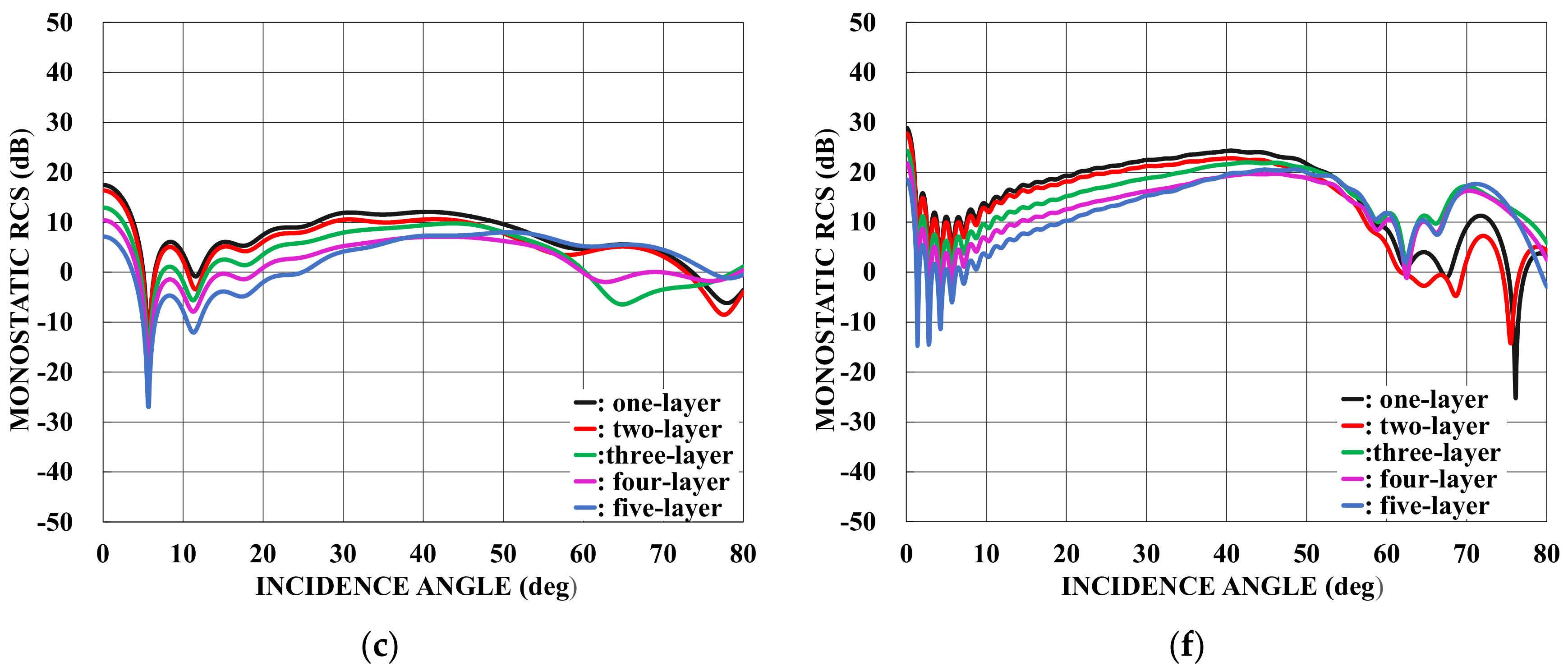
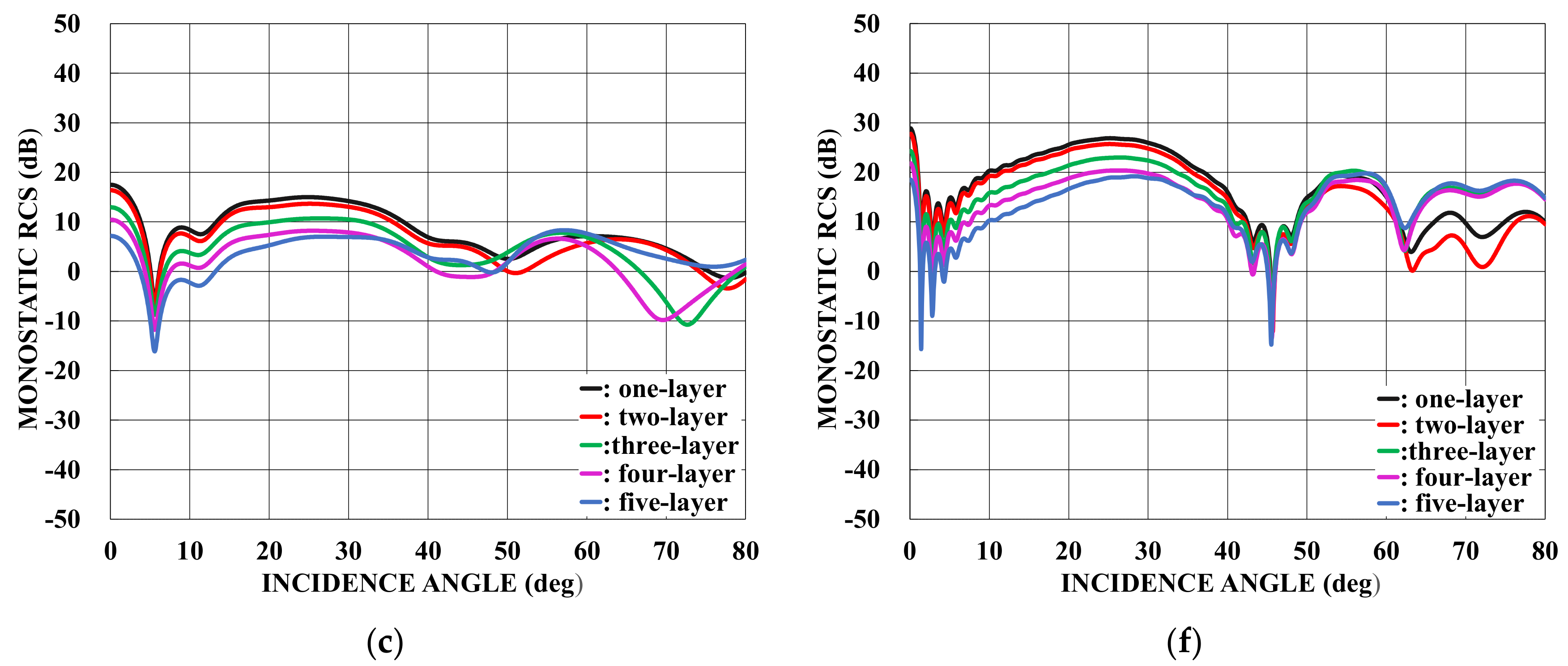
: one-layer material loading (regions II−V: vacuum). Applsci 13 03715 i002: two−layer material loading (regions III−V: vacuum). Applsci 13 03715 i003: three−layer material loading (regions IV−V: vacuum). Applsci 13 03715 i004: four−layer material loading (region V: vacuum). Applsci 13 03715 i005: five−layer material loading. (a) k b = 1.57 . (b) k b = 3.14 . (c) k b = 15.7 . (d) k b = 31.4 . (e) k b = 47.1 . (f) k b = 62.8 .
Applsci 13 03715 g002aApplsci 13 03715 g002b
Figure 3. Monostatic RCS [dB] versus incidence angle θ 0 for L 1 / 2 b = 1.0 ,     k t = 1.57 . Other particulars are the same as in Figure 2. (a) k b = 1.57 . (b) k b = 3.14 . (c) k b = 15.7 .(d) k b = 31.4 . (e) k b = 47.1 . (f) k b = 62.8 .
Applsci 13 03715 g003aApplsci 13 03715 g003b
Figure 4. Monostatic RCS [dB] versus incidence angle θ 0 for L 1 / 2 b = 3.0 ,   k t = 1.57 . Other particulars are the same as in Figure 2. (a) k b = 1.57 . (b) k b = 3.14 . (c) k b = 15.7 . (d) k b = 31.4 . (e) k b = 47.1 . (f) k b = 62.8 .
Applsci 13 03715 g004aApplsci 13 03715 g004b
Figure 5. Monostatic RCS [dB] versus incidence angle θ 0 for L 1 / 2 b = 5.0 ,     k t = 1.57 . Other particulars are the same as in Figure 2. (a) k b = 1.57 . (b) k b = 3.14 . (c) k b = 15.7 . (d) k b = 31.4 . (e) k b = 47.1 . (f) k b = 62.8 .
Applsci 13 03715 g005aApplsci 13 03715 g005b
Figure 6. Monostatic RCS [dB] versus normalized frequency kb for θ 0 = 0 ° ,   30 ° , and 60 ° , L 1 / 2 b = 1.0 ,   k t = 1.57 . Other particulars are the same as in Figure 2. (a) θ 0 = 0 ° . (b) θ 0 = 30 ° . (c) θ 0 = 60 ° .
Applsci 13 03715 g006aApplsci 13 03715 g006b
Figure 7. Comparison of the monostatic RCS [dB] versus incidence angle θ 0 between E- [46] and H-polarizations (this paper), L 1 / 2 b = 1.0 ,   k t = 1.57 . (a) k b = 3.14 . (b) k b = 62.8 .
Applsci 13 03715 g007
Figure 8. Comparison of the monostatic RCS [dB] versus normalized frequency kb between E- [46] and H-polarizations (this paper), L 1 / 2 b = 1.0 ,   k t = 1.57 . (a) θ 0 = 0 ° . (b) θ 0 = 60 ° .
Applsci 13 03715 g008
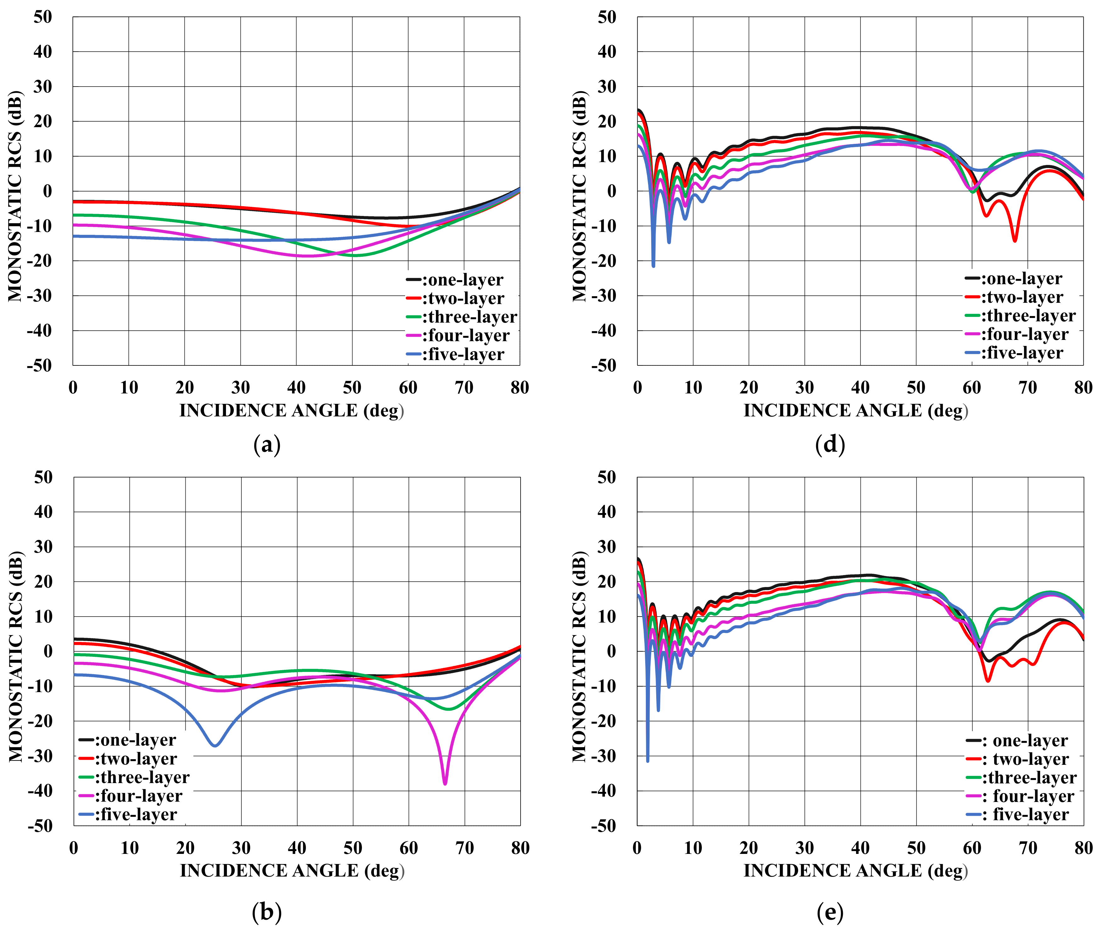
Disclaimer/Publisher’s Note: The statements, opinions and data contained in all publications are solely those of the individual author(s) and contributor(s) and not of MDPI and/or the editor(s). MDPI and/or the editor(s) disclaim responsibility for any injury to people or property resulting from any ideas, methods, instructions or products referred to in the content.

