1. Introduction
Open pit mines have a large, complex system, and the optimisation of their railroad transportation system is an important part of it. The optimisation of the railroad transportation system can play a crucial role in reducing production and operation costs, as well as in improving the production and organisational efficiency of mines. In recent years, the mining industry has been continuously improving its production and operation equipment, leading to increased automation levels and improved productivity. However, with the increased efficiencydespite these advancements, the bottleneck problems of the mine transport system have started to emerge, particularly with regard to the traditional routing optimisation planning models and algorithms that rely on a static road network analysis method.
Much research work, including mixed integer programming and dynamic programming, has been conducted to solve urban railroad transportation optimisation problems in the literature [
1,
2,
3,
4,
5,
6]. Compared with urban railway networks, mine railway networks have a limited amount of tracks, most of which are bidirectional single tracks. This leads to some particular problems, as follows.
Track allocation: Given most tracks are bidirectional single tracks, the transportation capacity is limited by the number of receiving and departure tracks, the number of siding/meetpoints, and the length of single tracks. Moreover, the capacity is also restricted by track maintenance.
Train conflict: For a bidirectional single-track, there are mainly two conflicts between trains. First, a predefined time difference is necessary to ensure safe operation when trains running in the same direction. Secondly, trains in opposite directions cannot be in the same segment at any time.
Given the problems stated above, the mine railroad scheduling problem is a complex optimisation problem, and the results under different decisions are far from each other. With the purpose of the less running time for all trains and maximizing the total amount of rolling stock, this paper proposes an integrated model by which to optimize train timetable and track allocation. The main contributions of this paper are listed as follows.
We first formulate a multiobjective optimisation problem for mine railway scheduling by introducing a set of mathematical constraints.
As the problem is NP-hard, we then devise a MIP-based solution to solve this problem in a real-time manner.
We finally conduct test cases to demonstrate the validity and effectiveness of the solution.
In the following sections,
Section 2 presents a review on the railway scheduling and train timetabling problems.
Section 3 introduces the system model and describes the mining railroad optimisation problem.
Section 4 provides the mathematical formulation for the objective and the set of constraints.
Section 5 presents a description of all the modules that constitute the developed solution, in order for all the readers to get an understanding of the entire process.
Section 6 presents a summary of the result for the tests carried out to evaluate the proposed solution.
Section 7 is dedicated to the conclusions.
2. Related Works
An enormous number of studies have been conducted on railway scheduling and train timetabling problems [
7,
8,
9,
10,
11,
12]. The research work can be classified into three main categories: the train scheduling and rescheduling problem, the periodic and nonperiodic timetabling problem, and the passenger train and freight train timetabling problem [
13].
Train scheduling is an offline problem that determines the arrival and departure times for trains at each station before the schedule is executed, e.g., [
14,
15,
16,
17,
18]. With a planned schedule, rescheduling is a real-time problem that aims to determine detailed train movements and timetables to minimize train deviations, e.g., [
19,
20,
21,
22]. Sanat et al. [
17] studied a train scheduling problem in a large national railway network, and presented two flexible heuristics based on a mixed integer program formulation for local optimisation to improve infrastructure utilization. Wang et al. [
18] studied the integration of train scheduling and rolling stock circulation planning under time-varying passenger demand for an urban rail transit line and proposed three approaches to solve the resulting multiobjective mixed-integer nonlinear programming problem to deliver both an irregular train schedule (i.e., departure and arrival times of all train services) and a rolling stock circulation plan (including entering/exiting depot operations of rolling stocks and connections between train services) simultaneously. Bersani et al. [
14] formalized demand-oriented scheduling and rescheduling models in order to propose a dynamic timetable, and proposed a min–max method with which to address operational constraints related to train capacity, train speed limits, train transfers, possible conflict in the track section use, with the main objective to minimize the travel time. Wang et al. [
20] proposed a train rescheduling optimisation model in the case of the vehicle breakdown on a metro line. Efficient rescheduling strategies including flexible short-turning and adding backup trains in particular are formulated into the model. Zhu and Goverde [
22] proposed a timetable rescheduling model to handle unexpected disruptions, where flexible stopping (i.e. skipping stops and adding stops) and flexible short-turning (i.e. full choice of short-turn stations) are innovatively integrated with three other dispatching measures: retiming, reordering, and cancelling.
Periodic timetabling requires that most or all train paths repeat in time with a certain period (e.g., 12 h), e.g., [
23,
24,
25,
26,
27]. However, as it becomes difficult to obtain effective periodic schedules when dealing with interruptions or conflicts (e.g., track maintenance), a nonperiodic timetable becomes more appropriate, e.g., [
28,
29]. Huang et al. [
23] integrated stop planning, service planning, and scheduling in a periodic timetabling problem and modelled it as a mixed integer linear programming formulation to minimize the average travel delay of passengers. They then developed a genetic algorithm supported by a scheduling heuristic to solve the problem for better scalability and efficiency. Polinder et al. [
24] considered a robust periodic timetabling problem—the problem of designing a periodic timetable that can easily be adjusted in case of small periodic disturbances—and developed a solution method for a parameterised class of uncertainty regions. Sparing et al. [
25] used the minimum cycle time of the periodic timetable as an indicator for stability, and defined an optimization problem with this minimum cycle time as the objective function to be minimized. They then proposed an optimization method to find a feasible periodic timetable that also ensures maximum stability for heterogeneous railway networks, which is capable of handling flexible train orders, running and dwell times, and overtaking locations. Schiewe et al. [
26] studied a periodic timetabling problem in public transportation planning, and developed an exact preprocessing method for reducing the problem size and a heuristic reduction approach in which only a subset of the passengers is considered. It provides upper and lower bounds on the objective value, such that it can be adjusted with respect to quality and computation time.
Because railways provide both passenger and freight services, there are naturally passenger train and freight train timetabling problems, e.g., [
30,
31,
32,
33,
34,
35,
36]. Mu and Dessouky [
33] introduced two mathematical formulations to cope with the rapidly increasing freight demand for railway transportation, and presented several heuristics that can significantly reduce the solution time of the exact method carried out by CPLEX, yet produce a satisfactory solution quality. Bešinović et al. [
31] introduced the integrated passenger and freight train timetable adjustment problem which handles both passenger as well as freight trains and developed a mixed integer linear programming model to simultaneously retime, reroute, and cancel trains in the network. Sato et al. [
35] studied freight train locomotive rescheduling when dealing with a disrupted situation in the daily operations in Japan, and solved the problem by changing the assignment of the locomotives to all the trains and considering their periodic inspections. Ozturk et al. [
34] considered a new concept for freight transport within the borders of a city with an urban rail transit system, and presented a decision support framework for the problem of urban freight movement by rail together with mathematical methods for the optimal distribution of goods. Given a transportation network with fixed routes for passenger trains and a set of freight trains (requests), Borndörfer et al. [
30] addressed a freight train routing problem, and calculated a feasible route for each freight train, such that the sum of all expected delays and all running times is minimal. Ursavas and Zhu [
36] studied decision-making problems that railway infrastructure managers face in a rail network with dedicated tracks and shared-use corridors, and analyzed the consolidation strategy for shared-use corridors, where the track serves passenger and freight.
These research lines are viewed from different perspectives but are not truly independent of each other. For example, passenger train scheduling is usually a periodic timetabling problem. Li et al. [
13] studied a nonperiodic freight train scheduling problem, in which a schedule is planned for freight trains and can be different during different periods of the day. The proposed method considers car flow transfer between consecutive trains and the shipment delivery time requirements. A tabu search algorithm is developed that extends the applicability of the proposed optimisation method for large-scale problems. Experiments on real-world instances of the Menghua railway indicate the effectiveness of the proposed algorithm.
3. Problem Description
Figure 1 shows a sample layout of mining railway network, where trains start from station A, travel via the tracks, load mine from load-out G, and return back to station A.
The mining railroad optimisation problem is to determine the best feasible timetable for a set of trains in order to load as many mines as possible. The related constraints are to satisfy restrictive operational constraints (e.g., track capacity, travel speed, safe distance, etc.) and to avoid possible conflicts when using each single track.
3.1. System Model
We define a physical network with a set of nodes S and a set of links W. The set S consists of switch stations (), and load-outs () in the physical network. is the set of links in physical network, where stands for link connecting node to node . The set W consists of mainline tracks (), siding tracks () and crossovers () in the physical network. For each link , let
be the capacity of where capacity is the maximum number of trains that can stand on the link at any point of time;
be the travel time from i to j, where f is the speed profile-based function; and
be the travel time from j to i, where f is the speed profile-based function.
In order to model the business operation of mine loading, for each load-out , let be the average loading time for a train.
Let be the set of time instants, where time is discretized into discrete time instants of length g minutes. For instance, if we take g = 5 then a period of 1 h would be represented by discrete set in our model.
3.2. Train Model
Let be the set of real trains travelling in the physical network . For each train , we will get the following set of inputs.
: Sequence of scheduled load-outs to visit;
: Scheduled departure time; and
: Scheduled departure location.
As we have a cyclical network and the train changes direction (turns back) after going to a load-out, in order to model this behaviour we will break down the train journey into different parts. Each part will be represented by a different model train. Thus, if a train m goes to n load-outs, its whole journey will be represented by a set of model trains, called , where each model train represents a specific segment of train m’s journey. Accordingly, one business rule will be added so that any model train can depart only after its predecessor has finished its journey.
For example, considering the case of a train
m starting from station A and going to two load-outs G1 and G2, its journey will be modelled as follows in
Table 1.
From now on, we will use the term “train” to refer to model train only, unless specified otherwise. Thus, for each train , we will have the following set of information.
: Scheduled departure time;
: Scheduled departure location node;
: Final destination node of the train, after which it will disappear from the network; and
: Predecessor train of train t.
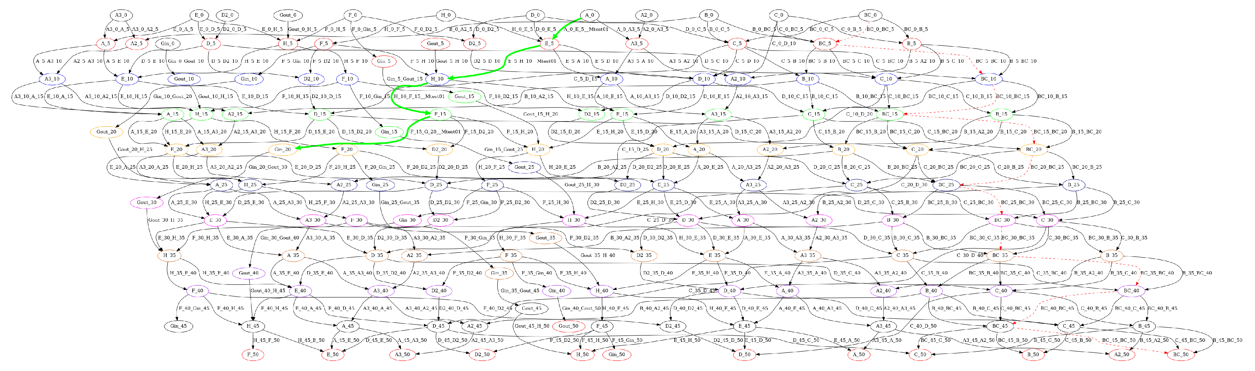
3.3. Time–Space Network
We here consider a time–space network , where N denotes the node set and A denotes the arc set. For each node , let be the set of all the outbound arcs of node i, and be the set of all the inbound arcs of node i.
Given a physical network , we then can construct the time–space network G as follows:
For each load-out in , we replace it with two separate node (entry node) and (exit node), and add a load-out link (, ) into W. Let be the set of load-out links. By splitting the entry and exit point nodes for each load-out, we ensure that trains are staying at load-out for the required loading time. At the same time, we replace the related inbound links to and the related outbound links to . Accordingly, we have , , and , where indicates the required loading time.
For each link with capacity , we break down the link into smaller links by adding dummy nodes into S and replacing the link with dummy links (with proportional travel time) as well. Note that after this operation, the capacity of each arc is 1. This operation guarantees that on every arc at any point of time only one train travels on that arc, which will in turn guarantee that trains maintain a safe headway separation while travelling in the same direction.
For each siding track , we add a siding node to S and replace the siding track with two separate arcs and . Let be the set of siding nodes. Accordingly, we have and . For each link , let be the set of identical arcs in A.
For each node , we add corresponding nodes in N. For each train , we add corresponding virtual source node in , where represents the source node where train t departs. We also add one sink into N, where represents the sink node where every train terminates its journey.
For each link
, we add following transit arcs into
:
and
For each link
, we then update
as follows:
For each siding node
, we add the following waiting arcs into
. In this way, we allow trains to wait/dwell on sidings:
For any load-out with loop capacity , we add waiting arcs between , for all . In this way, we allow trains to wait/dwell in the loops.
For each station node
, we add an arc from that node to the sink, signifying that this allows train cancellation in case of deadlock (i.e., we can cancel a train with a very high penalty). Thus, we add these train disappearing arcs into
:
For each train
, we add an arc from the source to the scheduled starting node of that train, and we add these starting arcs into
:
In all the above cases, whenever an arc is added to the time–space network, we also add this arc to the outbound arc set of node and to the inbound arc set of node .
5. Solution
The traditional approach to solve the above MIP problem is to use an offline scenario, which optimises the train schedule for a predefined time window. However, this approach is not suitable for the online scenario, where real-time updates are needed to keep up with the dynamic nature of the entire system. In the online scenario, the solving time often turns out to be unacceptable. For example, it may take several days to generate a train schedule for the next 24 h. It is not feasible to wait several days to generate a train schedule. Therefore, a more efficient solution framework is needed to handle the real-time requirements of the online scenario. We here propose a solution framework for the online scenario, which aims to address the limitations of the traditional approach by finding a balance between computational efficiency and optimisation accuracy.
In particular, we adopt the rolling-window approach. In this approach, a “rolling window” of time is defined, and the train scheduling problem is modeled as a MIP over this time horizon. The window is then moved forward in time, and the MIP is solved again for the new time period, taking into account the updated information. This solution framework can continuously monitor the train system, incorporate new information, and generate updated schedules in real time. This helps ensure that the trains are operating optimally, even in the face of unexpected events or changes.
As shown in
Figure 2, it runs iteratively. The cycle length is predefined (e.g., every 5 min), which is decided as per the business requirements (e.g., problem size, algorithm running time, etc.). For each cycle, it contains 4 steps as follows.
5.1. Preprocessing
In the preprocessing step, we use the current status as input and formulate the above MIP problem, in which complexity changes exponentially when variable size varies. To further reduce the running time, we adopt the following approaches to reduce the variables.
Initializing variables only for arcs on which train will travel: for each train, we only consider the reasonable arcs according to its destination. For example, in
Figure 3 the train
t is heading for load-out A. We then can set all the unreasonable variables (i.e., those variables associated to the arcs heading for load-out C) to 0.
Removing variables corresponding to unrealistic movements: consider the train
t in
Figure 4 going towards load-out, which is not allowed to move on track F. We then fix variables corresponding to such invalid movements to 0.
5.2. Solving MIP
In this step, we solve the formulated MIP problem for the coming scheduling window via mathematical optimisation solver (e.g., Gurobi, Xpress, Cplex, etc.). The choice of a proper scheduling window size depends on the specific requirements and constraints of the problem, as well as the available computational resources. To better utilize the solver, we also integrate more strategies as follows.
Warm start: supply hints to help the solver find an initial solution, which consists of pairs of variables and values, known as a warm start. The hints may come from soft business rules or human experience.
Solver tuning: use offline data to tune the solver, and adopt the solver setting for the online running. As shown in
Table 2 , we tuned parameters for both Gurobi and Xpress.
5.3. Postprocessing
The postprocessing step is a crucial part of the optimisation solution. After getting the MIP results, we then need to translate the math-style results into a schedule of trains’ movements. This process involves combining individual trains with their related predecessor trains to get complete movements. As shown in
Table 1, we need to combine the results of
,
,
to get the schedule of train
m.
5.4. Simulation/Execution
In this step, we validate the schedule further through simulation and add more details, such as maintenance allocation. This step helps ensure that the schedule is accurate and feasible before it is executed. Finally, we communicate the detailed schedule to the trains, triggering an actual execution. This involves updating the trains’ schedules in real-time so that they can follow the optimal path and arrive at their destinations as efficiently as possible. This step is critical for ensuring that the solution is implemented correctly and that the trains’ movements are optimised as planned.


