
A Model for Oxygen Transport from Blood in Microvessels to Tissue

Department of Chemical and Biological Engineering, American University of Sharjah, Sharjah P.O. Box 26666, United Arab Emirates
Appl. Sci. 2023, 13(6), 3805; https://doi.org/10.3390/app13063805
Submission received: 6 February 2023
/
Revised: 11 March 2023
/
Accepted: 11 March 2023
/
Published: 16 March 2023
(This article belongs to the Section Applied Biosciences and Bioengineering)
Abstract
:Oxygen is vital for cellular energetics and metabolism in the human body. Blood transports oxygen to the tissues with hemoglobin in red blood cells playing a key role in the transportation of oxygen. To account for the Fåhraeus and Fåhraeus–Lindqvist effects, we use Haynes marginal zone concept, which subdivides each microvessel into a cell free layer surrounding a core region of uniform red blood cells concentration. The marginal zone concept is used to develop a steady state model for the transport of oxygen from blood to tissue where chemical reaction of oxygen occurs to produce energy. The approach is based on fundamentals of fluid flow and mass transfer in the two zones while accounting for the role of hemoglobin in the transport process and including mass transfer and chemical reaction in the tissue to produce energy using the Krogh cylinder concept. In contrast to transport modeling of solutes such as glucose, the present model includes the key role of hemoglobin in the transport of oxygen from blood to tissue. The model is analytical and provides analytical expressions for the oxygen level profiles in the blood cell free layer, the core zone, and the Krogh cylinder. The results are found to agree with published results in the literature for oxygen transport from blood in capillary size microvessel to its Krogh tissue cylinder. The model is not restricted to transport from capillaries and includes transport of oxygen from microvessels to tissue in general. Extensions of the model include further investigations in the case where changes in the blood microvessel or red blood cells occur due to pathological conditions.
1. Introduction
Flow in microvessels of diameter less than about 500 μm has a larger discharge hematocrit than the tube hematocrit (hematocrit ratio less than one) (Fåhraeus effect) and a decreasing apparent viscosity as capillary diameter decreases (Fåhraeus–Lindqvist effect) [1,2,3,4,5,6]. Both effects are explained by Haynes marginal concept [7]. The model divides the capillary side into a cell-free annular layer and a core region containing plasma and the red blood cells. A review of the marginal zone concept can be found in [8,9,10,11]. Shear induced migration and elastic stress induced models are considered in [12,13,14,15] using the concept introduced in [16,17], and [18,19,20,21,22], respectively. Particulate (mesoscale) models are discussed in [23,24], and viscoelastic models are reviewed in [23].
Krogh mass transport of oxygen in tissue [25], review and extensions of the Krogh model including mass transport in the capillary surrounded by the Krogh tissue cylinder can be found in [3,23,26,27,28,29] and the references therein. Several numerical models considered oxygen transport in capillaries while accounting for the particulate nature of RBCs, assuming different shapes of RBCs: spherical, cylindrical, and parachute form [30,31,32,33,34] with different frames of reference. A simplified analytical model is also provided in [34]. Computational models are introduced for the transport of oxygen (i) based on a one-dimensional (1D) model for microvascular network and a 3D model for porous tissue in [35] and (ii) using a computational method based on incomplete boundary conditions to model microvascular networks in [36].
The model of Fournier [3] for oxygen transport accounts for oxygen transport in capillaries using a uniform velocity profile while accounting for transport of oxygen in plasma and the role of hemoglobin in the transport process, with Krogh model used for transport by diffusion and oxygen consumption in the tissue side. On the other hand, the particulate models account for mass transport in microvessels with each cross-sectional area containing no more than one RBC. In a microvessel, there is a cell-free layer in which no RBCs are present, with a core region where RBCs concentrate. This segregation is considered in the present analysis of oxygen transport. The present model accounts for mass transport in both zones while including the role of hemoglobin in transport of oxygen in the core region. In addition, non-uniformity of the velocity profiles in the two zones and transport of oxygen in the tissue side are included in the present analysis of oxygen transport from blood to tissue. In contrast to a previously published model for solute transport (such as glucose) from blood to tissue [37], the present model includes the key role of hemoglobin in the transport of oxygen.
2. Governing Equations
2.1. Blood Flow Model
The model used is based on the Haynes marginal theory [3,7,11]. The annular zone is the cell-free layer, and the core zone contains plasma and red blood cells (Figure 1).
The main results are summarized, and results are needed for the mass transfer model of oxygen from blood to the surrounding tissue Krogh cylinder.
The hydrodynamic model is a continuum model using the no-slip boundary condition at the capillary wall (r = R), finite shear stress at the axial location (r = 0), and continuity of the velocity and the shear stress at the interface between the annular layer and the core region (r = ri).
The model yields the following velocity profiles in the fully developed flow region: vc in the core region, va in the annular layer, and vi at the interface
where
Pgr is the pressure gradient and μc and μa denote the core region and annular layer viscosities, respectively. Other relations include the following relation for the volumetric flow rate Q, and the average velocity v*
The apparent viscosity is provided by
with the following relations reported in [3]
where HC is the core region hematocrit and temperature T is in Kelvin.
The required values of HC and the discharge hematocrit HD can be obtained using the following relations
where HT is the tube hematocrit and σ denotes ri/R.
2.2. Mass Transfer Model
Oxygen is mainly transported by hemoglobin Hb with n molecules bound to Hb. At equilibrium, Hill’s equation is used to provide hemoglobin saturation Y as a function of partial pressure of oxygen, pO2 [3], and Hill’s constant n
where, at a partial pressure of oxygen equal to p50, the binding sites of hemoglobin are half filled.
The governing equations for dissolved oxygen balance in the core region plasma is given by
where cc and Dc are the free oxygen concentration in the core and the diffusion coefficient in the core region, respectively, and R is the rate of conversion to oxygenated hemoglobin.
Neglecting diffusional effects as in [3], the conservation equation of oxygenated hemoglobin can be written as
where cHbO is the hemoglobin-bound oxygen concentration.
Adding Equations (10) and (11) and using the chain rule yields [3]
where Dc is estimated using Maxwell equation [3,38]
We can also express equations using partial pressure = cc/αa, where αa denotes oxygen solubility, to get
Using Hill’s equation yields [3]
where n and p50 are equal to 2.34 and 26 mm Hg, respectively, and cc,sat is the maximum concentration for oxygen (with four oxygen molecules of oxygen bound and a maximum concentration of hemoglobin in blood of 2200 μM) is 8800 μM [3].
The mass transfer of dissolved oxygen in the annular zone (cell-free layer) is governed by
where ca and Da denote the dissolved oxygen concentration and diffusion coefficient in the annular zone, respectively. Dissolved oxygen levels can be expressed in terms of oxygen partial pressure using Henry’s law [3]. The above equation yields
In the tissue side, the partial pressure profile in the Krogh model where mass transfer is limited to the Krogh tissue cylinder of radius rT surrounding the microvessel [3,23,25,26,27,28]. The governing equation is
where cT and DT are the oxygen dissolved concentration and diffusion coefficient in the tissue side, respectively, and Γ is the rate of consumption of oxygen. Dropping the diffusional term in the z-direction and setting the flux to zero at rT, to exclude mass transfer across the different Krogh tissue cylinders, yields the Krogh-Erlang solution [25,27]
This gives the following in terms of oxygen partial pressure
where αT denotes oxygen solubility in tissue.
The following boundary conditions express the continuity of the partial pressures of oxygen
3. Solution
We seek the following solution
where oxygen pressures are linear function of z, and φc, φa, and φT are functions of r. Continuity at the interfaces requires equality of the slopes: bc = ba = bT = b, with subscripts dropped. In Equation (25), φ simply represents the deviation of oxygen partial pressures from the average oxygen partial pressure in blood . Substituting the relevant expressions for oxygen partial pressure in Equation (31) into Equations (14) and (17) yields the following ordinary differential equations
subject to the following boundary conditions
Integrating Equations (26) and (27) using boundary conditions (28) and (29) yields
where mav is an average value for m. Using boundary condition (30) provides a relationship between the two remaining unknowns b and K
The constant b needed to find the drop in the partial pressure of oxygen per unit change of length in the axial direction, and a mass balance on oxygen is performed in the annular zone between z and z + Δz
Using Equations (31) and (32) yields after substitution into Equation (34), integration and rearrangement
In order to determine φi, we apply the overall mass balance to the annular zone between 0 and z
Using Equation (34) reduces the above equation to
Substituting for the expressions of va and φa given in Equations (1) and (32), and integrating gives
where λ = R/ri = 1/σ and
4. Computational Procedure and Results
The calculations require expressions for Aa and Ac. The following results are derived from Equations (1)–(3)
Using the values σ = 0.9, HT = 34.2%, previously used in [37] to study glucose transport from blood to tissue, yields: HC = 42.2%, μc/μa = 1.947, HD = 40.0%, and μapp/μa = 1.469 using Equations (7) and (6) at T = 300 K, and (5) and (4) sequentially.
The expression for slope b can be written in a more convenient form as
where mav is calculated using Equation (15) and an average value for taken as , which obviously requires simple trial and error calculations, by successive substitutions to get mav. The expressions for and vi are obtained using Equation (1)
The profiles for the deviations from the pressure at the interface are given by the following expressions:
where K is given by
where ξT = rT / R. The value of is used to get the oxygen partial pressure at the two zones interface
where f is given by
The case of metabolic consumption of oxygen in an islet of Langerhans is considered in [3]. The data, reported in [3], is a capillary blood flow rate of about 7 nL/min for a tissue perfusion rate qb (capillary blood flow rate over Krogh tissue volume) and about 4 mL/cm3 min. The data used are listed in Table 1 included the relevant references.
The solubilities in Table 1 are calculated using the values in mL O2/cm3 mm Hg and the O2 molar volume at 36.9 °C in [33]. Using the data in Table 1, and the above–mentioned value of μc/μa = 1.947 obtained for σ = 0.9 and HT = 34.2% (HD = 40.0%), yields the results summarized in Table 2. Using the perfusion rate of about 4 mL/cm3 min used in [3] and the Krogh tissue cylinder volume as a function of R, rT and L, the outer radius of the Krogh cylinder rT is found to be about 24 μm.
Using Equations (45) and (46) provides the values for φ (r = 0) and φ (R). Combining Equations (46) and Equation (45) (applied at r = R) gives the following expression for φT:
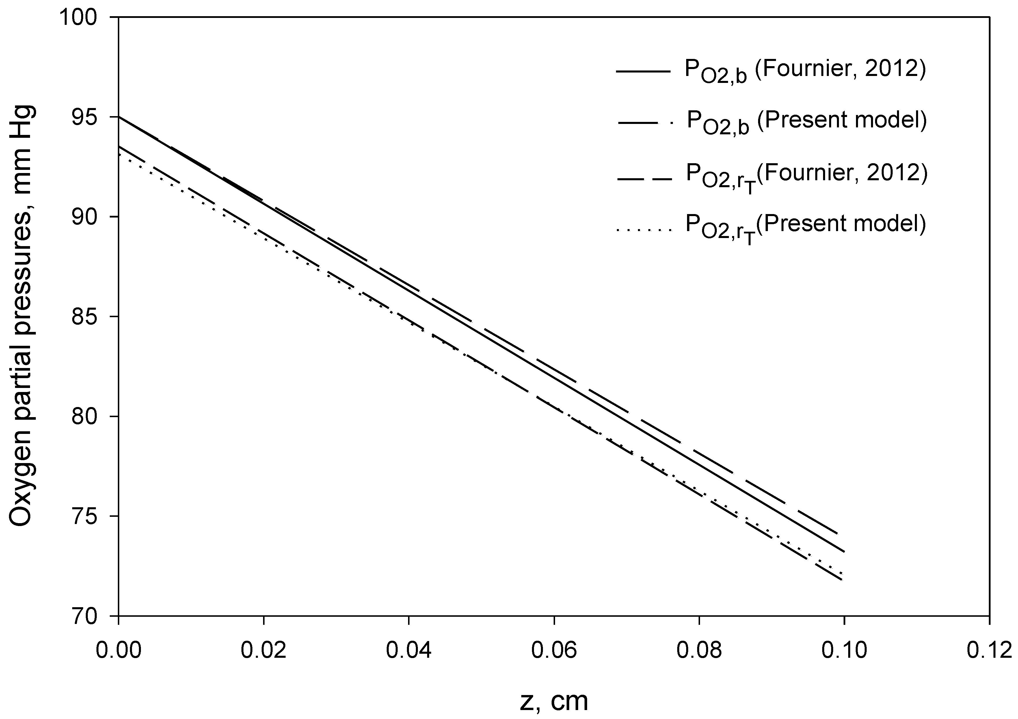
The results obtained in Table 2 (using the data in Table 1) are used to plot the oxygen partial pressures profiles in Figure 2. As expected, the oxygen partial pressure profiles show a drop in the z direction due to consumption of oxygen in the tissue. The average oxygen partial pressure in blood is higher than the oxygen partial pressure at the outer radius of the Krogh cylinder due to mass transfer resistance to oxygen transport from blood to tissue. The results compare favorably with those in [3], as seen from Figure 2.
The case of anoxia starts when the oxygen pressure at rT is zero at z = L (critical case):
In vitro experiments providing the required data for comparison with the present model are recommended for future investigations.
5. Conclusions
Segregation of red blood cells in microvessels is accounted for in the present model on the basis of fundamentals of fluid flow and mass transfer and including metabolic consumption of oxygen in tissue, using Haynes marginal zone and Krogh cylinder concepts. The key role of hemoglobin is included in mass transfer of oxygen. In addition, velocity gradients in the cell-free zone and the core region inside the microvessel are accounted for in the transport of oxygen model. The final expressions are analytical. The results are found in good agreement with the results of Fournier [3] for oxygen transport from blood in capillary size microvessel to surrounding tissue. Although an average value of m was considered over all the capillary length as in [3], it is possible to subdivide the capillary length into small segments and use an average value for m over each interval for more accuracy. The model is not restricted to transport of oxygen from capillaries and includes transport of oxygen from blood in microvessels to tissue in general.
Funding
The work in this paper was supported, in part, by the Open Access Program from the American University of Sharjah. This paper represents the opinions of the author and does not mean to represent the position or opinions of the American University of Sharjah.
Institutional Review Board Statement
The research does not involve human participants and/or animals.
Data Availability Statement
All data used are mentioned in the manuscript. The relevant references are mentioned and listed.
Conflicts of Interest
The author declares that he has no competing interests.
References
- Fåhraeus, R. The suspension stability of blood. Physiol. Rev. 1929, 9, 241–274. [Google Scholar] [CrossRef]
- Fåhraeus, R.; Lindqvist, T. The viscosity of the blood in narrow capillary tubes. Am. J. Physiol. 1931, 96, 562–568. [Google Scholar] [CrossRef]
- Fournier, R.L. Basic Transport Phenomena in Biomedical Engineering; CRC Press: Boca Raton, FL, USA, 2012. [Google Scholar]
- Goldsmith, H.L.; Cokelet, G.R.; Gaehtgens, P.; Fåhræus, R. Evolution of his concepts in cardiovascular physiology. Am. J. Physiol. Heart Circ. Physiol. 1989, 257, H1005–H1015. [Google Scholar] [CrossRef] [PubMed]
- Toksvang, L.N.; Berg, R.M.G. Using a classic paper by Robin Fåhraeus and Torsten Lindqvist to teach basic hemorheology. Adv. Physiol. Educ. 2013, 37, 129–133. [Google Scholar] [CrossRef] [PubMed] [Green Version]
- Secomb, T.W.; Pries, A.R. Blood viscosity in microvessels: Experiment and theory. Comptes Rendus Phys. 2013, 14, 470–478. [Google Scholar] [CrossRef] [Green Version]
- Haynes, R.F. Physical basis of the dependence of blood viscosity on tube radius. Am. J. Physiol. 1960, 198, 1193–1200. [Google Scholar] [CrossRef]
- Pries, A.R.; Neuhaus, D.; Gaehtgens, P. Blood viscosity in tube flow: Dependence on diameter and hematocrit. Am. J. Physiol. Heart Circul. Phys. 1992, 263, H1770–H1778. [Google Scholar] [CrossRef] [Green Version]
- Sharan, M.; Popel, A.S. A two-phase model for flow of blood in narrow tubes with increased effective viscosity near the wall. Biorheology 2001, 38, 415–428. [Google Scholar]
- Sriram, K.; Intaglietta, M.; Tartakovsky, D.M. Non-Newtonian flow of blood in arterioles: Consequences for wall shear stress measurements. Microcirculation 2014, 21, 628–639. [Google Scholar] [CrossRef] [Green Version]
- Chebbi, R. Dynamics of blood flow: Modeling of the Fåhræus–Lindqvist effect. J. Biol. Phys. 2015, 41, 313–326. [Google Scholar] [CrossRef] [Green Version]
- Weert, K.V. Numerical and Experimental Analysis of Shear-Induced Migration in Suspension Flow. Master’s Thesis, Eindhoven University, Eindhoven, The Netherlands, 2005. [Google Scholar]
- Mansour, M.H.; Bressloff, N.W.; Shearman, C.P. Red blood cell migration in Microvessels. Biorheology 2010, 47, 73–93. [Google Scholar] [CrossRef] [PubMed]
- Chebbi, R. Dynamics of blood flow: Modeling of Fåhraeus and Fåhraeus-Lindqvist effects using a shear-induced red blood cell migration model. J. Biol. Phys. 2018, 44, 591–603. [Google Scholar] [CrossRef] [PubMed]
- Chebbi, R. A two-zone shear-induced red blood cell migration model for blood flow in microvessels. Front. Phys. 2019, 7, 206. [Google Scholar] [CrossRef] [Green Version]
- Leighton, D.T.; Acrivos, A. The shear-induced migration of particles in concentrated suspension. J. Fluid Mech. 1987, 181, 415–439. [Google Scholar] [CrossRef]
- Phillips, R.J.; Armstrong, R.C.; Brown, R.A. A constitutive equation for concentrated suspensions that accounts for shear-induced particle migration. Phys. Fluids 1992, 4, 30–40. [Google Scholar] [CrossRef]
- Moyers-Gonzalez, M.; Owens, R.G.; Fang, J. A non-homogeneous constitutive model for human blood. Part 1. Model derivation and steady flow. J. Fluid Mech. 2008, 617, 327–354. [Google Scholar] [CrossRef] [Green Version]
- Moyers-Gonzalez, M.A.; Owens, R.G. Mathematical modelling of the cell-depleted peripheral layer in the steady flow of blood in a tube. Biorheology 2010, 47, 39–71. [Google Scholar] [CrossRef]
- Dimakopoulos, Y.; Kelesidis, G.; Tsouka, S.; Georgiou, G.C.; Tsamopoulos, J. Hemodynamics in stenotic vessels of small diameter under steady state conditions: Effect of viscoelasticity and migration of red blood cells. Biorheology 2015, 52, 183–210. [Google Scholar] [CrossRef] [Green Version]
- Mavrantzas, V.G.; Beris, A.N. Modelling the rheology and the flow-induced concentration changes in polymer solutions. Phys. Rev. Lett. 1993, 69, 273–276, Erratum in Phys. Rev. Lett. 1993, 70, 2659. [Google Scholar] [CrossRef]
- Tsouka, S.; Dimakopoulos, Y.; Mavrantzas, V.; Tsamopoulos, J. Stress-gradient induced migration of polymers in corrugated channels. J. Rheol. 2014, 58, 911–947. [Google Scholar] [CrossRef]
- Arciero, J.C.; Causin, P.; Malgaroli, F. Mathematical methods for modeling the microcirculation. AIMS Biophys. 2017, 4, 362–399. [Google Scholar] [CrossRef]
- Bessonov, N.; Sequeira, A.; Simakov, S.; Vassilevski Yu Volpert, V. Methods of blood flow modelling. Math. Model. Nat. Phenom. 2016, 11, 1–25. [Google Scholar] [CrossRef] [Green Version]
- Krogh, A. The number and distribution of capillaries in muscles with calculations of the oxygen pressure head necessary for supplying the tissue. J. Physiol. 1919, 52, 409–415. [Google Scholar] [CrossRef]
- Popel, A.S. Theory of oxygen transport to tissue. Crit. Rev. Biomed. Eng. 1989, 17, 257–321. [Google Scholar]
- Goldman, D. Theoretical models of microvascular oxygen transport to tissue. Microcirculation 2008, 15, 795–811. [Google Scholar] [CrossRef] [Green Version]
- Truskey, G.A.; Yuan, F.; Katz, D.F. Transport Phenomena in Biological Systems; Pearson: Upper Saddle River, NJ, USA, 2010. [Google Scholar]
- Hellums, J.D. The resistance to oxygen transport in the capillaries relative to that in the surrounding tissue. Microvasc. Res. 1977, 13, 131–136. [Google Scholar] [CrossRef]
- Federspiel, W.J.; Popel, A.S. A theoretical analysis of the effect of the particulate nature of blood on oxygen release in capillaries. Microvasc. Res. 1986, 32, 164–189. [Google Scholar] [CrossRef]
- Eggleton, C.D.; Vadapalli, A.; Roy, T.K.; Popel, A.S. Calculations of intracapillary oxygen tension distributions in muscle. Math. Biosci. 2000, 167, 123–143. [Google Scholar] [CrossRef]
- Vadapalli, A.; Goldman, D.; Popel, A.S. Calculations of oxygen transport by red blood cells and hemoglobin solutions in capillaries. Artif. Cells Blood Substit. Immobil. Biotechnol. 2002, 30, 157–188. [Google Scholar] [CrossRef]
- Lucker, A.; Weber, B.; Jenny, P.A. Dynamic model of oxygen transport from capillaries to tissue with moving red blood cells. Am. J. Physiol. Heart Circ. Physiol. 2015, 308, H206–H216. [Google Scholar] [CrossRef] [Green Version]
- Lücker, A.; Secomb, T.W.; Weber, B.; Jenny, P. The relative influence of hematocrit and red blood cell velocity on oxygen transport from capillaries to tissue. Microcirculation 2017, 24, e12337. [Google Scholar] [CrossRef] [PubMed] [Green Version]
- Possenti, L.; Cicchetti, A.; Rosati, R.; Cerroni, D.; Costantino, M.L.; Rancati, T.; Zunino, P. A mesoscale computational model for microvascular oxygen transfer. Ann. Biomed. Eng. 2021, 49, 3356–3373. [Google Scholar] [CrossRef] [PubMed]
- Celaya-Alcala, J.T.; Lee, G.V.; Smith, A.F.; Li, B.; Sakadzi, S.; Boas, D.A.; Secomb, T.W. Simulation of oxygen transport and estimation of tissue perfusion in extensive microvascular networks: Application to cerebral cortex. J. Cereb. Blood Flow Metab. 2021, 41, 656–669. [Google Scholar] [CrossRef] [PubMed]
- Chebbi, R. An analytical model for solute transport from blood to tissue. Open Phys. 2022, 20, 249–258. [Google Scholar] [CrossRef]
- Bird, R.B.; Stewart, W.E.; Lightfoot, E.N. Transport Phenomena; Wiley: New York, NY, USA, 2007. [Google Scholar]
Figure 1.
Schematic of oxygen transport from a microvessel to its Krogh tissue cylinder. The two zones introduced by Haynes are shown: a cell-free layer surrounding a core zone where RBCs concentrate.
Figure 1.
Schematic of oxygen transport from a microvessel to its Krogh tissue cylinder. The two zones introduced by Haynes are shown: a cell-free layer surrounding a core zone where RBCs concentrate.
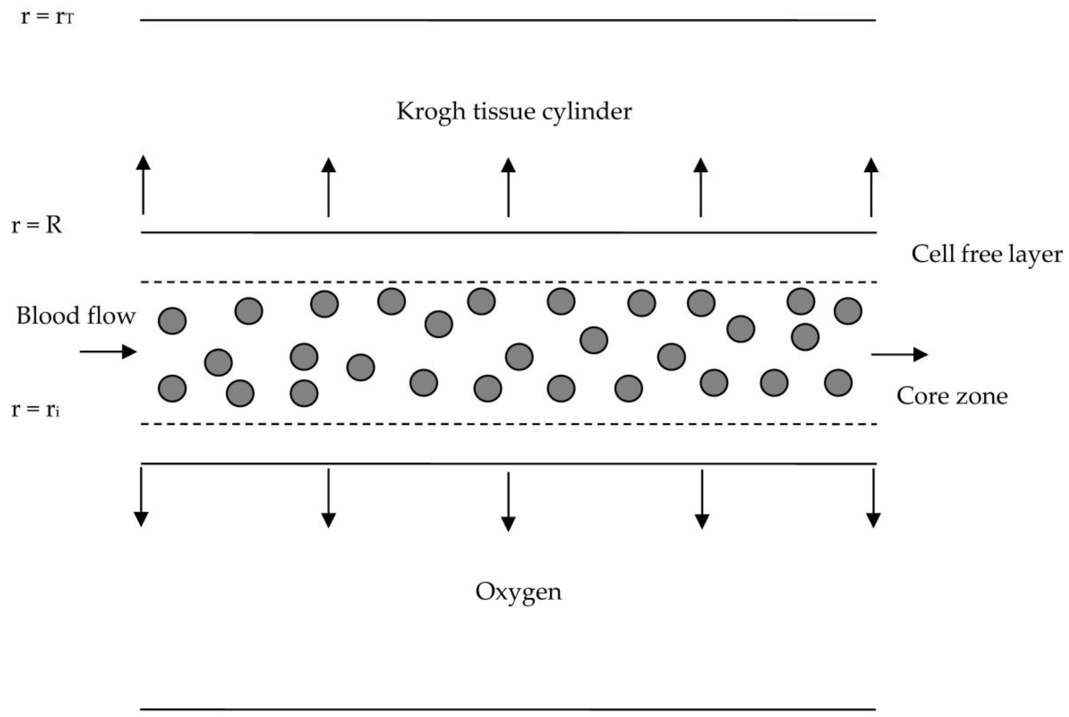
Figure 2.
Profiles for dissolved oxygen profiles in blood and at the Krogh tissue cylinder radius [3].
Figure 2.
Profiles for dissolved oxygen profiles in blood and at the Krogh tissue cylinder radius [3].

Table 1.
Data used for oxygen transport from blood flow in a capillary and comparison with (3).
| Property | Symbol | Value | Reference |
|---|---|---|---|
| Da | Diffusion coefficient in plasma | 2.18 × 10⁻⁵ cm2/s | [33] |
| DRBC | Diffusion coefficient in RBCs | 9.5 × 10⁻⁶ cm2/s | [33] |
| DT | Diffusion coefficient in tissue | 2.41 × 10⁻⁵ cm2/s | [33] |
| 2 R | Capillary diameter | 10 μm | Table 5.1 [3] |
| L | Length | 1000 μm | Table 5.1 [3] |
| Γ | Rate of oxygen consumption in tissue | 20 μM/s | Chapter 6 [3] |
| Average oxygen partial pressure in blood at z = 0 | 95 mm Hg | Chapter 6 [3] | |
| Q | Volume flow rate of blood | 7 nL/min | Chapter 6 [3] |
| αa | Oxygen solubility in plasma | 1.110 μM O2/mm Hg (2.82 × 10⁻⁵ mL O2/cm3 mm Hg) | [33] |
| αT | Oxygen solubility in tissue | 1.516 μM O2/mm Hg (3.85 × 10⁻⁵ mL O2/cm3 mm Hg) | [33] |
Table 2.
Results for oxygen transport using Table 1 for μc/μa = 1.947 and σ = 0.9. (HD = 40.0%).
Table 2.
Results for oxygen transport using Table 1 for μc/μa = 1.947 and σ = 0.9. (HD = 40.0%).
| Symbol | Value |
|---|---|
| v* | 0.149 cm/s |
| rT | 24 μm |
| AcR2 | −0.224 cm/s |
| AaR2 | −0.436 cm/s |
| vi | 0.0829 cm/s |
| va | 0.0415 cm/s |
| b | 210.88 mm Hg/cm |
| K | −2.013 mmHg |
| Dc | 1.60 × 10⁻⁵ cm2/s |
| bAaR4/Da | −1.06 mm Hg |
| bAcR4/Dc | −0.740 mm Hg |
| ΓR2/(αaDa) | 0.207 mm Hg |
| ΓR2/(αTDT) | 0.137 mm Hg |
| φi | 0.0840 mm Hg |
| φa at R | −0.1555 mm Hg |
| φT at rT | −1.875 mm Hg |
| pO2,b at z = L | 73.91 mm Hg |
| mav | 12.33 |
Disclaimer/Publisher’s Note: The statements, opinions and data contained in all publications are solely those of the individual author(s) and contributor(s) and not of MDPI and/or the editor(s). MDPI and/or the editor(s) disclaim responsibility for any injury to people or property resulting from any ideas, methods, instructions or products referred to in the content. |
© 2023 by the author. Licensee MDPI, Basel, Switzerland. This article is an open access article distributed under the terms and conditions of the Creative Commons Attribution (CC BY) license (https://creativecommons.org/licenses/by/4.0/).
Share and Cite
MDPI and ACS Style
Chebbi, R. A Model for Oxygen Transport from Blood in Microvessels to Tissue. Appl. Sci. 2023, 13, 3805. https://doi.org/10.3390/app13063805
AMA Style
Chebbi R. A Model for Oxygen Transport from Blood in Microvessels to Tissue. Applied Sciences. 2023; 13(6):3805. https://doi.org/10.3390/app13063805
Chicago/Turabian StyleChebbi, Rachid. 2023. "A Model for Oxygen Transport from Blood in Microvessels to Tissue" Applied Sciences 13, no. 6: 3805. https://doi.org/10.3390/app13063805
Note that from the first issue of 2016, this journal uses article numbers instead of page numbers. See further details here.