Article

Vertebral Center Points Locating and Cobb Angle Measurement Based on Deep Learning

School of Mechanical and Automotive Engineering, Shanghai University of Engineering Science, Shanghai 201620, China
*
Author to whom correspondence should be addressed.
These authors contributed equally to this work.
Appl. Sci. 2023, 13(6), 3817; https://doi.org/10.3390/app13063817
Submission received: 7 February 2023 / Revised: 13 March 2023 / Accepted: 14 March 2023 / Published: 16 March 2023

Abstract

:
Traditional manual measurement of Cobb angle is a time-consuming process and leads to different results. To address this issue, this paper proposes a deep learning-based method of locating the vertebral center points. The whole X-ray can be input into the network for prediction, without worrying about the detection of cervical vertebrae with similar characteristics to the thoracic and lumbar vertebrae. First, key points predicting and noise points filtering operations are employed to obtain vertebral center points for fitting. Then, the spine curve is fitted, and the slope of the normal line of the spine curve is adjusted according to an empirical formula. Finally, the Cobb angle allowed by the error is calculated. Through the reliability analysis of the traditional manual measurement method and the automatic detection method in this paper, ICC (intraclass correlation coefficient) with the two observers was 0.897 and 0.901, respectively, and MAD (mean absolute deviation) was 3.13° and 3.04° respectively. This indicates that the automatic detecting method by computer has good reliability. Therefore, this method can be used to detect scoliosis quickly and effectively.

1. Introduction

Scoliosis is a physical condition characterized by a lateral curvature of the spine, usually defined as a curve on a standing radiograph of the spine measuring at least 10° [1]. Adolescent Idiopathic scoliosis is the most common form seen in clinical practice, accounting for nearly 80% of cases. The prevalence is estimated to be 1.3/1000 in children under 8 years of age and 1.8/1000 in children over 8 years of age [2]. This condition can lead to a variety of problems, including obvious body shape deformities, decreased chest volume, impaired spinal movement and breathing, decreased trunk balance, increased incidence of back pain, serious aesthetic problems, activity limitation and decreased quality of life [3,4,5]. The traditional method of diagnosing a curved spine determines the end vertebra on the X-ray film, draws the line at the corresponding end vertebra, and measures the spine curvature according to the drawn lines. This method is time-consuming, laborious, and vulnerable to the professional level of the medical surveyors, subjective factors, and other influences, leading to specific discrepancies in the results.
In recent years, with the rapid development of deep learning and image processing, scoliosis measurement methods have also advanced significantly. Zhang et al. [6] proposed a method of Cobb angle measurement that employed Canny edge detection, fuzzy Hough transform (FHT) and spine edge structure detection. The peak value in Hough space was selected and the line that coincided with the upper and lower edges of the vertebra was determined according to the constraint conditions of the shape of the vertebra, and, finally, the Cobb angle was calculated. Jhilam et al. [7] proposed a method to calculate Cobb angle. Firstly, the end vertebrae (the vertebra with the greatest inclination in the scoliosis) are manually selected and then denoised and histogram equalized. Then the canny edge detection operator is applied to the enhanced image to detect the edge of the vertebrae used to measure the Cobb angle. Finally, the line detection is carried out through Hough transform and the Cobb angle is calculated. Mehmood et al. [8] employed intervertebral distance and positioning to differentiate cervical vertebrae from the spine. The X-ray image is preprocessed through histogram equalization, Canny edge detection, etc. Then the C3-C7 cervical region of interest (ROI) was manually selected. After the generalized Hough transform (GHT) and fuzzy C-means clustering, the center points of vertebrae are detected, and the center points of the intervertebral disc between vertebrae are obtained. The distance between two adjacent vertebrae was calculated and their centroids were found, thus obtaining the region of each vertebra. Affine transformation was then carried out on the lines passing through the centroid and connecting the two vertebrae, and vertical separation lines were found on these centroids, finally obtaining the boundary of the vertebra. Al-Bashir et al. [9] segmented each column of pixel points of the preprocessed spine x-ray by the thresholding, extracted the contour using Canny edge detection, calculated the vertebral center points, and fitted the spine curve. Zhang et al. [10] proposed a Cobb angle measurement method which requires users to select vertebrae from the upper to the lower vertebrae via mouse operation. For each selected vertebra, a 150 × 150-pixel rectangle for each selected vertebras created and sent to the DNN for predicting the slope of the vertebra. Subsequently, the tilt angle of the two end vertebrae are then detected and the sum of the absolute values of the tilt angles is calculated as the Cobb angle. Sun et al. [11] calculated Cobb angle using a key point detection method. They proposed Structured Support Vector Regression (S2VR), which directly estimates corner coordinates and Cobb angles by expressing prediction as a multi-output regression task. The Cobb angle measurement method proposed by Wang et al. [12] proposed a Cobb angle measurement method which firstly determines the UEV and LEV of scoliosis segments. Then, they mark UEVEL and LEVEL on the film using the measurement program built in PACS (Picture Archiving and Communication System), and calculate Cobb angle. Chen et al. [13] proposed an Adaptive Error Correction Network(AEC) to directly calculate Cobb angle. AEC first uses two methods to estimate Cobb angle: LandmarkNet, which is used to indirectly calculate the Cobb angle by regressing corner points, and AngleNet, which is used to directly regress Cobb angle. Then, the errors of the two estimated Cobb angles are adaptively offset by an alternative error correction network using extrapolation. Sun et al. [14] first detected the C7-L5 vertebrae from an X-ray image of the whole spine, reducing the resolution from 1750 × 3064 pixels to 768 × 1152 pixels and cropping the area to 512 × 512 pixels. This cropped area was then sent to a corner detection model, from which the Cobb angle was calculated according to the corner points. Although these methods have achieved specific results in the automatic detection of scoliosis, their stability and robustness could still be improved, as they are affected by the initial image quality. Moreover, the data sets used by these methods are not anteroposterior X-ray images of the entire spine. In actual use, requiring the X-ray images need to be cropped or manually boxed selected for actual use.
This paper proposes a deep learning-based algorithm for detecting vertebral center points, tailored to the needs of scoliosis in practical applications. The cervical vertebrae, sacrum, and coccyx are filtered by detecting four anchor points through a parallel network. Heatmap is used to regress the desired vertebral body center points, fit the spine curve, adjust the normal slope of the spine curve, and calculate the accurate Cobb angles. This method does not require cropping or other operations on the X-ray image, and can automatically detect the Cobb angles.

2. Manual Measurement of Scoliosis

The Cobb angle measurement is a commonly used method to assess the severity of scoliosis. It is determined by measuring the angle formed at the intersection of two perpendicular lines drawn at the end of vertebrae on the X-ray image of the spine [1]. Figure 1 shows the definition of Cobb angle. After the determined end vertebrae (the vertebrae with the greatest inclination to the concave side of scoliosis) are determined, draw parallel lines on the upper edge of the upper end vertebra and the lower edge of the lower end vertebra. The angle between these two lines is the Cobb angle [15].
The size of Cobb angles plays an important role in the subsequent diagnosis and treatment. Depending on the age and remaining growth potential of the patient, it is determined whether to observe the treatment, use a brace or perform a surgical procedure [16,17,18]. The Cobb angle measurement results may vary due to the patient’s body position during the X-ray and the skill level of the medical surveyors, with an error range of typically 3–5 degrees.
The traditional manual measurement method is prone to differences in the professional level of the measurers and subjective factors, and is also inefficient, taking about ten minutes for a spine X-ray measurement. To address this, this paper proposes a deep learning network-based method to predict the vertebral center points, fit the spine curve, determine the end vertebra according to the curve slope variations, and finally obtain the Cobb angles. Compared to the traditional manual measurement method, this proposed method is more efficient, rigorous, and faster.

3. Materials and Methods

3.1. Network Structure

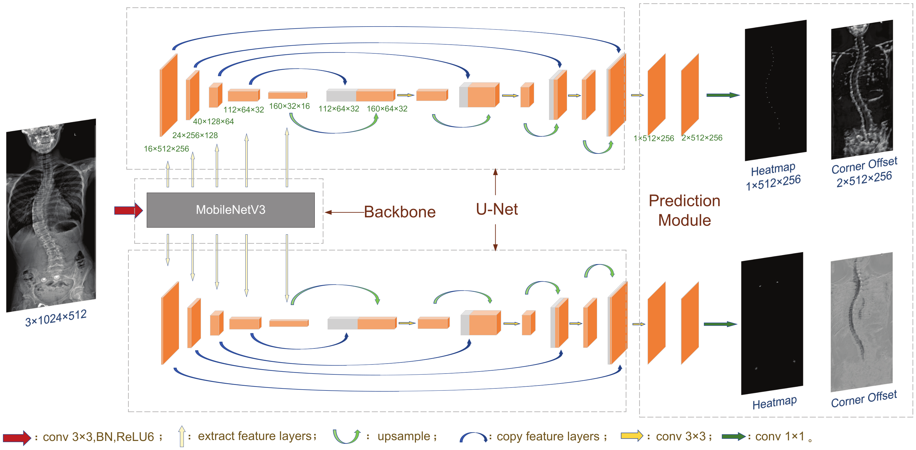
The network structure for detecting vertebral center points consists of three parts, with a lightweight network MobileNetV3 [19] as the Backbone for feature extraction. This Backbone network can generate five feature layers with different resolutions and a different number of convolution kernels which contain the information on different scales of the input X-ray image.
The middle part of the network is U-Net [20], which is specially designed for medical datasets with large resolution and small size. The left half of the network is a shrinking network for extracting information, where the size of the feature image is constantly decreasing. It consists of four blocks with the same structure, each containing several convolution layers and a Max Pool layer. The 4 blocks are downsampled by the convolution kernel to obtain a feature layer respectively. In this paper, MobileNetV3 is employed to generate the four feature layers. The right half of U-Net is an expansion path that is symmetrical to the left. The expansion path block is firstly sampled from the previous feature layer to the size of the corresponding feature layer in the shrinking network, and then copied and spliced with the feature layer in the channel number dimension. After convolution, the number of channels is made the same as the number of channels in the feature layer. During the information extraction process, the contraction path will continuously reduce the resolution of the feature layer. In contrast, the expansion path can retain high-level abstract semantic information in the upsampling process and concatenate feature maps corresponding to the contraction path, thus making it essential for more accurate localization.
The final prediction module of the network utilizes the idea of CenterNet [21], employs a 3 × 3 convolution layer to transform the feature map to the desired dimension, and adopts the 1 × 1 convolution to generate a heat map of vertebral center points and center offset. The center offset can accurately detect the vertebral center points based on the heatmap.
The human spine consists of seven cervical vertebrae, twelve thoracic vertebrae, five lumbar vertebrae, one sacrum, and one coccyx. To distinguish the cervical vertebrae, which generate 85% of the noise with similar features to the thoracic and lumbar vertebrae, a parallel network is established to detect four anchor points. These anchor points are located at the first group of the clavicle and hip bone, respectively. As shown in Figure 2, the network structure is designed to accurately predict the center points of the vertebrae.
The network structure parameters are few, and the low-semantic information in the spine X-ray can be extracted through the Backbone of the model. The contraction and expansion paths of the U-Net structure in the middle of the network are also the encoding and decoding processes which extract more features of the image in the encoding process and gradually restore the spatial dimension in the decoding process, fusing the previously extracted features to achieve accurate target positioning. The network’s structural characteristics and the transfer learning method enable the model to be trained and converged on a custom dataset of spine X-rays with only a few hundred images.

3.2. Loss Calculation

3.2.1. Heat Map Loss

Since the detected object is the center point of vertebrae, the annotation data should be preprocessed to avoid an all-zero matrix while calculating the loss. Heat map regression [22,23] is usually utilized to regress key points with high accuracy and convergence speed. The heat map consists of a series of two-dimensional Gaussian disks, with different weights are given to the regions near the actual value, where the closer it is to the actual value, the greater the weight. The pixel values in the Gaussian disk are all positive, and the point with the pixel value of 1 is the actual value of the marked point. The values in the Gaussian disk can be derived from e x 2 + y 2 2 σ 2 , where x and y determine the range of the Gaussian circle, and the size of the detected object determines σ . Since the scales of the input images are the same, σ = 1 is taken for vertebral center points and the two locating points at the clavicle and σ = 1.5 for the two points at the hip bone in this experiment.
The heatmap loss is calculated using the following Focal Loss function [24]:
L H e a t m a p = 1 N i = 1 h j = 1 w ( 1 p i j ) α l o g ( p i j ) y i j = 1 ( 1 y i j ) β ( p i j ) α l o g ( 1 p i j ) o t h e r s
where N is the total number of all pixels on the heat map, h and w are the height and width of the heat map, respectively, p i j is the predicted score of a pixel, y i j represents the predicted score of pixels on the real heat map augmented by a non-normalized Gaussian function, and α and β are hyper-parameters that affect the contribution of pixels. In this experiment, we choose α = 2 and β = 4 , which are consistent with the literature [21].

3.2.2. Center Offset

The prediction of center offset acts as a correction to the location of the predicted vertebral center points. After the input image passes through the convolutional layer in the network, the output heat map size is smaller than the original image, resulting in errors when the points on the heat map are mapped back to the original image. Thus, a center offset should be introduced to adjust the position of the predicted point as:
o i = x i n x i n , y i n y i n
where x i , y i represents the coordinates of the point, and o i is the center offset.
During the training process, the s m o o t h L 1 l o s s [25] is utilized to regress center offset, which can easily generate a sparse matrix, quickly return to the required features, and is more robust than the L 1 L o s s . The formula is as follows:
L o f f s e t s = 1 n i N S m o o t h L 1 L o s s ( o i , o i ^ )
where o i and o i ^ are the actual and predicted values of offsets, respectively, N is the number of pixels.

3.3. Network Training

We first train the Backbone on the public dataset Mini-ImageNet to extract low-semantic information, and then train the rest layers on the X-ray dataset. Experiments show that the key points prediction results are good provided there’s no cover at vertebrae. Although one anchor point will be missed for some X-rays with poor image quality, it will not affect the results of subsequent noise filtering.

3.3.1. Experimental Environment

Experimental platform configuration: The GPU used in this experiment is GTX3060, and the video memory is 12 GB. The running software is PyCharm in Anaconda virtual environment, and the pytorch version is 1.9.0.
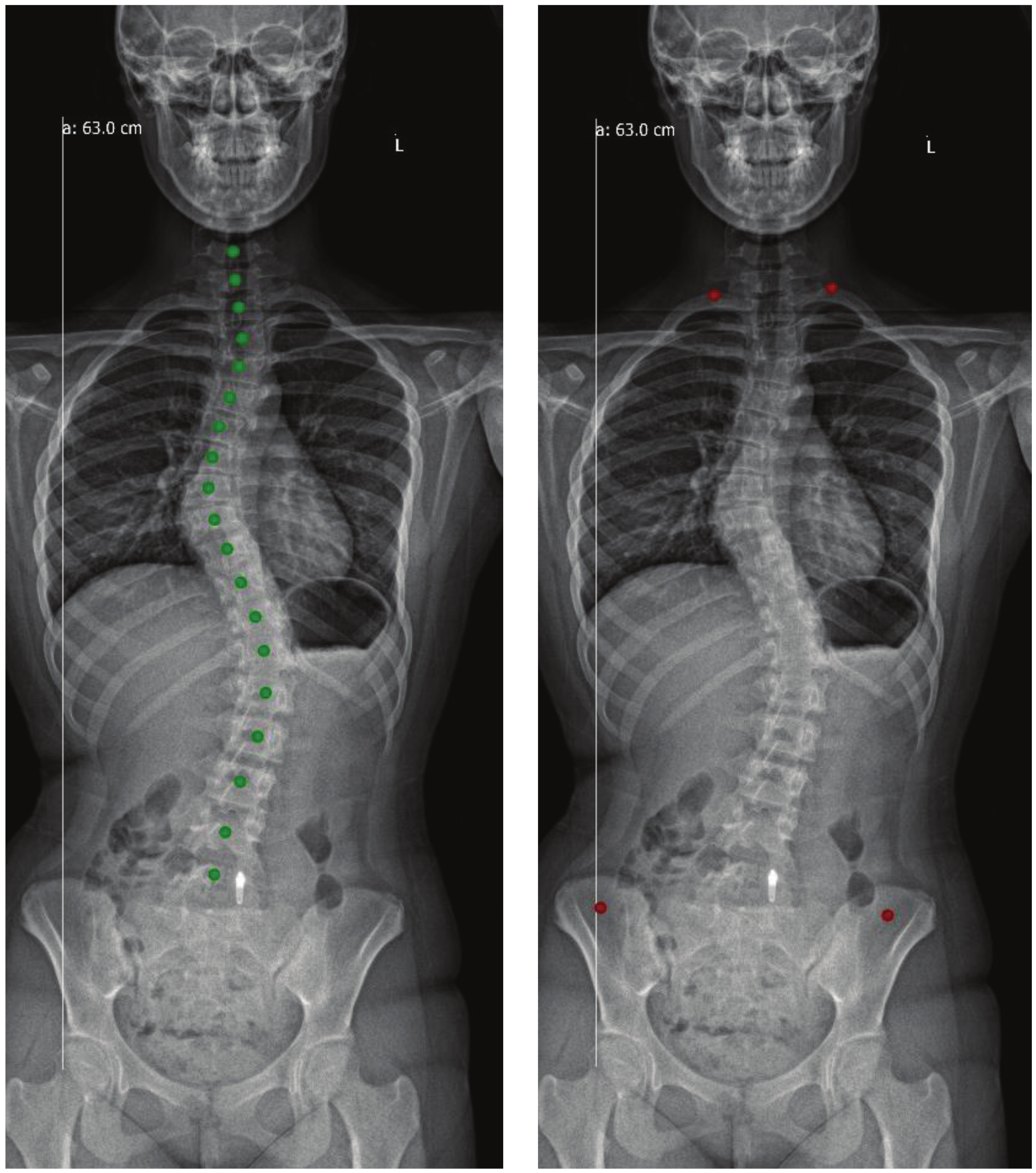
Dataset:In this experiment, the mini-ImageNet public dataset is utilized for training the Backbone, consisting of 60,000 annotated images, including 48,000 for training-set and 12,000 for validation-set, with a total of 100 categories. The custom dataset comprises 420 X-slices provided by Carespine company. Of these, 323 are adopted for training, 57 for validation, and 40 for testing, all of which are annotated in JSON file format. The X-rays are not intercepted; the images contain features such as the skull, cervical spine, thoracic spine, lumbar spine, hip bone, and sacrum. Since the thoracic, lumbar, and cervical vertebrae have a very high similarity, the center points of the cervical vertebrae with clear outlines in the X-ray are also marked in addition to marking the centers of the 17 vertebrae. An example of data set annotation is shown in Figure 3, with the left side representing the vertebral center points annotation, and the right side representing the four anchor point annotation.

3.3.2. Training Process

In this experiment, the Backbone was first trained on the Mini-ImageNet dataset until the loss was stable and no longer dropping significantly.
To normalize and expand the dataset, and improve the model’s generalization ability, routine data processing and data enhancement were performed on the custom dataset before training the entire network, including resetting image resolution, normalization, photometric distortion, random crop, random horizontal flip, and random rotation angle.
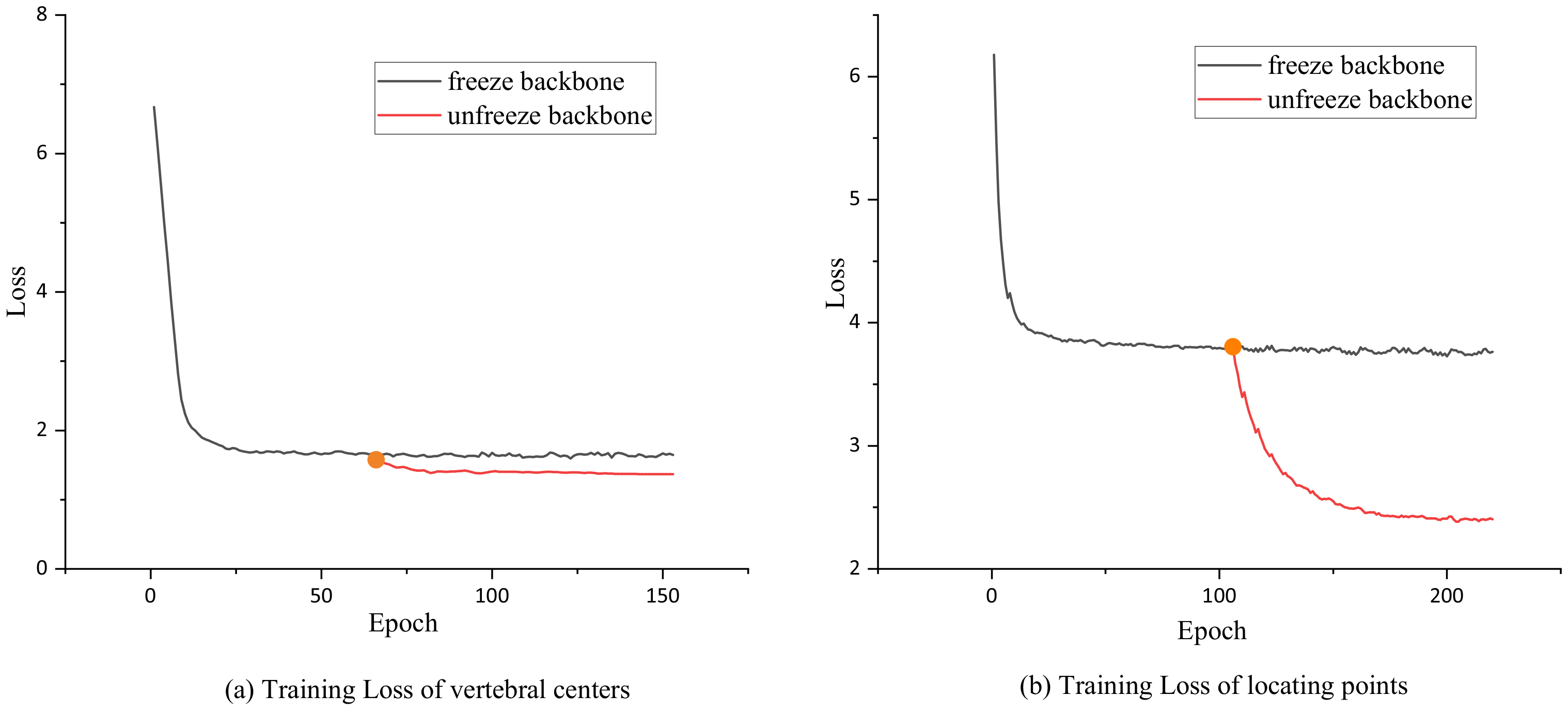
The Backbone weights are initially frozen while the feature layer weights of the network are trained. When the loss stops decreasing, the Backbone weights are unfrozen, and the entire network is trained until the model converges. The two parallel routes are trained to obtain two sets of weights, employed to predict the vertebral center points and the four anchor points, respectively. The Adam optimizer [26] was adopted during training, and the learning rate decays exponentially. Figure 4 shows the changes in the loss of vertebral center points and anchor points before and after freezing the Backbone weights during training. As can be seen in the figure, the loss further decreased when the backbone was unfrozen during training.
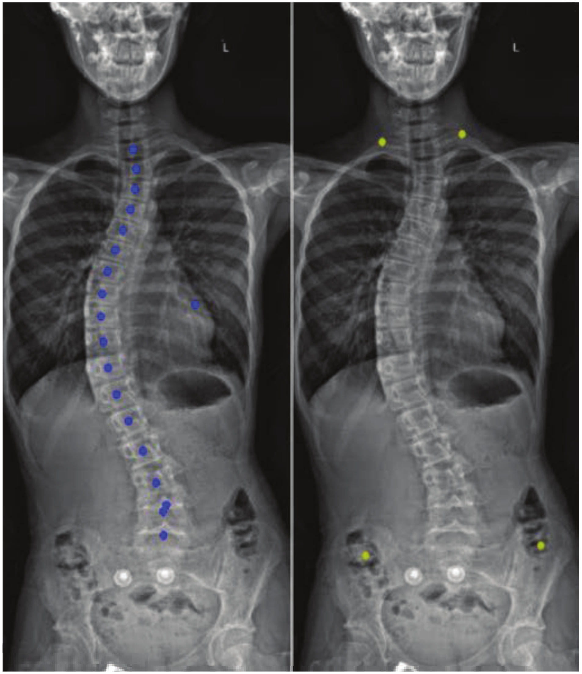
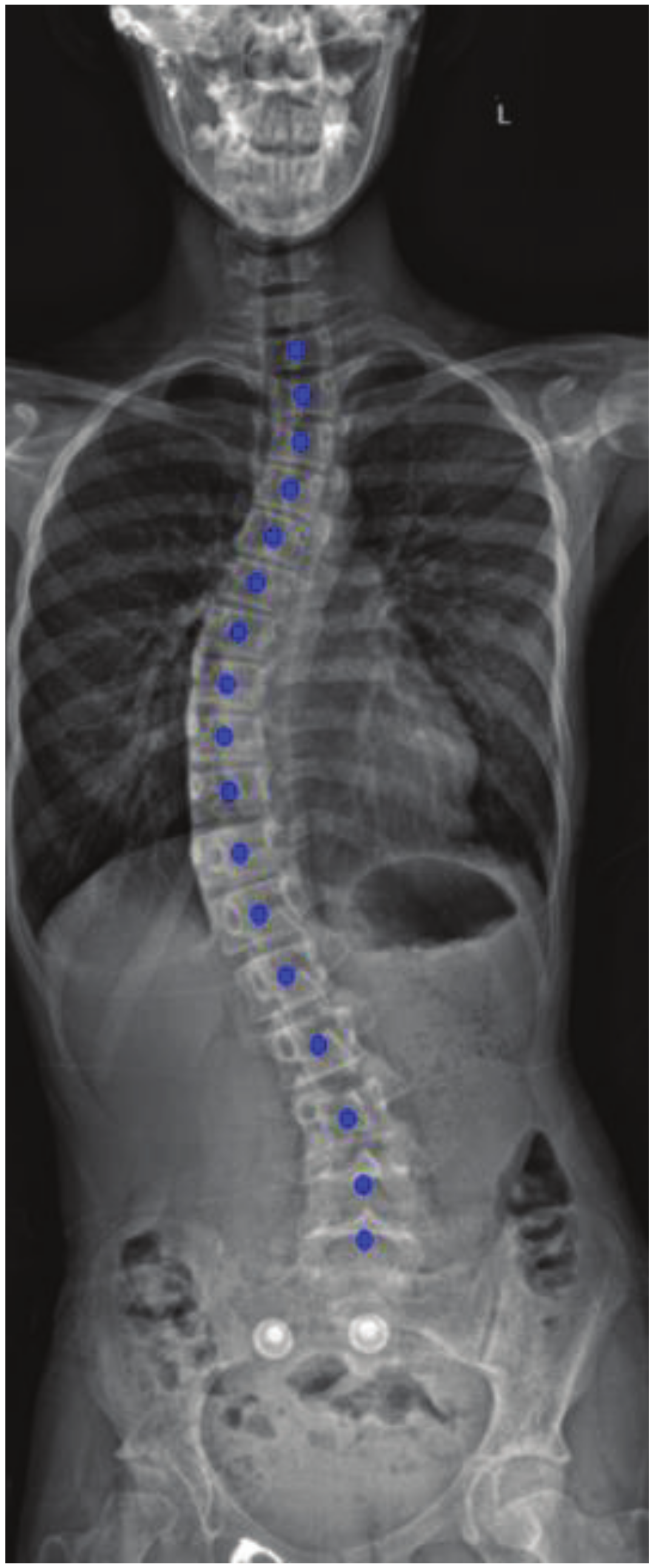
The trained weights are used to predict spine X-rays, and the results are shown in Figure 5. Experiments showed that the key point detection effect was effective. However, there were some noise points in the prediction of the vertebral center points, which should be filtered before using the predicted points for curve fitting.

3.4. Post-Processing

3.4.1. Noise Removal

The above experiment shows that the prediction of the vertebral center points and the point used for positioning is accurate. However, some pictures have individual noise points in the key points predicted by some pictures, and different filtering methods are used to deal with them. For noises with close distances, such as two prediction points on the same spine, filtering can be done by taking the maximum prediction score of the pixels within a certain pixel range of each prediction point.
For noise points with a large distance, the absolute value of the difference between the abscissa of each point and the mean value of the abscissa of all predicted points is calculated. If it exceeds the given threshold, it is considered a noise point and should be filtered. As shown in Figure 6, the key points of the obtained spine are all in the center of the vertebral body without noticeable deviation. Curve fitting can then be performed based on these 17 vertebral center points.

3.4.2. Spine Curve Fitting and Cobb Angle Calculation

The Cobb angle is a measure of the degree of scoliosis. The end vertebra of a lateral curvature is used to determine the Cobb angle. In this experiment, the end vertebra is determined by fitting a 7th-degree polynomial to the 17 vertebral center points predicted by the network, using the y-coordinate as an independent variable. The Cobb angle is then calculated by taking the included angle between the upper and lower end vertebrae, determined by the slope of the normal line at the fitted curve.
The experiment found that the upper and lower edges of the vertebrae are not parallel to the normal line at the fitted curve due to the interaction force between the vertebrae. Furthermore, a positive correlation was observed between the error and the fitted spine curve. Thus, the angle error is calculated using Formula (4) to correct the normal slope.
Δ i = d i | d i | · l o g α ( 1 + d i )
where i is the index of the spine center, is the correction factor, d is the slope of the tangent line, and is the angle error. In the above correction process, the angle between the normal line and the positive direction of the X-axis is subtracted from the correction degree calculated by this formula. Figure 7 shows the results before and after correction:

4. Results

To evaluate the model performance and Cobb angle measurement results, we calculated the model parameters, mean absolute percentage error (MAPE), and FPS were evaluated on the 40 X-piece test-set. The results are summarized in Table 1. The MAPE was calculated as:
MAPE = 1 N n · N n | θ g t θ p r e d θ p r e d | · 100 %
where N is the number of samples, n is the number of lateral curvatures in a sample, and θ g t and θ p r e d are the actual and predicted values of the Cobb angle, respectively.
As shown in Table 1, the MAPE of the proposed method is comparable to the first two models, thile the parameter quantity is significantly reduced and the frame per second (FPS) is higher.
To demonstrate the impact of utilizing locating points and correction formula on measurement results, we relabeled the central point of the vertebrae in the dataset and only labeled 17 vertebrae for detection. As shown in Table 2, direct training and prediction of the central points of 17 vertebrae on the full spine X-ray resulted in large errors and low accuracy in selecting end vertebrae. Notably, the error corresponding to the proximal thoracic (PT) was the largest due to the similarity between cervical vertebrae characteristics and those of the detected thoracic and lumbar vertebrae, leading to the model detecting cervical vertebrae and causing significant deviation in end vertebrae selection, thereby affecting Cobb angle measurements. However, with the use of locating points and correction formula, accuracy rates were significantly improved. Thus, the proposed method of utilizing locating points can effectively minimize the impact of cervical vertebrae and other features on X-ray, while the use of empirical formula can enhance measurement accuracy.
To further verify the effectiveness of the proposed method, we conducted reliability analysis on the above test-set. Table 3 records ICC (intraclass correlation coefficient) and MAD (mean absolute deviation) of the two surveyors. It can be seen that the intra-observer results of the two observers are 0.951 and 0.958 respectively, with MADs 2.24 and 2.16 respectively. The ICCs between the two measurements are 0.940 and 0.942, and the MADs are 2.61 and 2.55, respectively. These results demonstrate that manual measurement is reliable.
Table 4 records the intra-group correlation coefficients between the automatic detection method in this paper and the results obtained by two surveyors using the manual measurement method. The analysis between automatic Cobb angle detection method and manual measurement yielded an ICC of 0.897 and 0.902, respectively, and a MAD of 3.13 and 3.04, respectively. This indicates that the automatic detection method has good reliability.

5. Discussion

Given the time-consuming and imprecise nature of the traditional manual approach to measuring Cobb angle, there is a growing trend towards utilizing computers to automate the Cobb angle measurement process on X-rays images. The Cobb angle is calculated based on 12 thoracic vertebrae and 5 lumbar vertebrae. However, the human spine additionally comprises cervical vertebrae, the hip bone and the sacrum, the latter of which share many similar characteristics to the thoracic and lumbar vertebrae, thus posing a significant challenge to the computer’s ability to detect vertebrae. Drawing on the traditional image processing method [6,7,8,9], which necessitates the selection of parameters, an incorrect configuration can lead to erroneous outcomes. Furthermore, it is less effective for the processing of complex images, e.g., those containing noise or weak edges, and comparatively low treatment efficiency. The methods based on deep learning [10,13,14] have achieved certain results in vertebrae detection. However, the datasets used by these methods are all cropped X-ray images of the spine, or the user needs to box-select the spine to exclude the information on the X-ray that will interfere with the detection of the spine. In particular, the cervical vertebrae, which are very similar to the 17 vertebrae (12 thoracic vertebrae and 5 lumbar vertebrae) to be detected, will significantly impact the prediction results and cannot be automatically distinguished from thoracic vertebrae and lumbar vertebrae after prediction. Therefore, these methods cannot accurately and automatically detect scoliosis without cropping or manually frame-selecting the X-rays of the input network.
This paper presents a method that utilizes anteroposterior X-ray images of the entire spine without cropping. In order to resolve the problems mentioned, in addition to predicting the center point of each vertebra, the network also predicts four positioning points, thereby allowing for the filtering of points that are predicted to be above the first thoracic vertebra and below the last lumbar vertebra on the full spine X-ray images and thus realize the automatic detection of the Cobb angle. The consistency between observers and within observers was analyzed using the Intraclass Correlation Coefficient (ICC) with 95% confidence interval (CI). It was concluded that the automated measurement method was reliable.
This study has several limitations. First, there is limited research on the selection of the end vertebrae, which may be biased for spines with slight scoliosis due to the close slope between adjacent vertebrae. Secondly, this paper has not conducted an in-depth investigation into the discrepancies between the measurement results of proximal thoracic (PT), main thoracic (MT) and thoracolumbar (TL) curves. Finally, this paper did not investigate the classification of scoliosis based on the automatically detected Cobb angle. These issues will be addressed in our future research.

6. Conclusions

Accurate measurement is essential for scoliosis diagnosis. However, the current manual measurement method is inefficient, subjective, and unstable. Additionally, current computer-aided detection of the Cobb angle requires manual cropping or frame selection of X-ray images, which cannot achieve full automation. This paper proposes a deep learning-based vertebral center points localization algorithm, which fits the spine curve according to the predicted key points to calculate the Cobb angle. Experiments demonstrate that this method has good robustness and practicability, and its specific advantages are as follows:
(1)
It can predict the entire X-ray input without the need for cropping while only keeping the thoracic and lumbar vertebrae that need to be predicted, which meets the practical application requirements.
(2)
It is more stable, rigorous, and rapid than traditional manual measurement.
(3)
The number of network parameters is small, saving memory resources and improving the detection speed while ensuring the accuracy.

Author Contributions

Z.Z.: funding acquisition, project administration, writing—review and editing; J.Z.: conceptualization, methodology, writing—original draft; C.Y.: formal analysis, methodology. All authors have read and agreed to the published version of the manuscript.

Funding

This work was partly supported by Program of Shanghai Academic/Technology Research Leader (22XD1433500).

Institutional Review Board Statement

Not applicable.

Informed Consent Statement

Not applicable.

Data Availability Statement

Author elects to not share data.

Acknowledgments

The authors wish to acknowledge Liduan Wang from Shanghai Sinan Satellite Navigation Technology Co., Ltd. for providing the experimental equipment and funding.

Conflicts of Interest

The authors declare no conflict of interest.

References

  1. Alman, B. Overview and Comparison of Idiopathic, Neuromuscular, and Congenital Forms of Scoliosis. In The Genetics and Development of Scoliosis; Kusumi, K., Dunwoodie, S.L., Eds.; Springer: Cham, Switzerland, 2018; pp. 73–79. [Google Scholar]
  2. Haleem, S.; Nnadi, C. Scoliosis: A review. Paediatr. Child Health 2018, 28, 209–217. [Google Scholar] [CrossRef]
  3. Du, C.P.; Yu, J.D.; Zhang, J.Q.; Jiang, J.; Lai, H.; Liu, W.; Liu, Y.; Li, H.; Wang, P. Relevant areas of functioning in patients with adolescent idiopathic scoliosis on the International Classification of Functioning, Disability and Health: The patients’ perspective. J. Rehabil. Med. 2016, 48, 806–814. [Google Scholar] [CrossRef] [PubMed] [Green Version]
  4. Lang, C.D.; Wang, R.J.; Chen, Z.M.; He, S.; Zou, Q.; Wu, J.; Zhu, X. Incidence and Risk Factors of Cardiac Abnormalities in Patients with Idiopathic Scoliosis. World Neurosurg. 2019, 125, 824–828. [Google Scholar] [CrossRef] [PubMed]
  5. Li, X.; Guo, H.; Chen, C.; Tan, H.; Lin, Y.; Li, Z.; Shen, J. Does Scoliosis Affect Sleep Breathing? World Neurosurg. 2018, 118, 946–950. [Google Scholar] [CrossRef] [PubMed]
  6. Zhang, J.; Lou, E.; Le, L.H.; Hill, D.L.; Raso, J.V.; Wang, Y. Automatic Cobb measurement of scoliosis based on fuzzy Hough Transform with vertebral shape prior. J. Digit. Imaging 2009, 22, 463–472. [Google Scholar] [CrossRef] [PubMed] [Green Version]
  7. Mukherjee, J.; Kundu, R.; Chakrabarti, A. Variability of Cobb angle measurement from digital X-ray image based on different de-noising techniques. Int. J. Biomed. Eng. Technol. 2014, 16, 113–134. [Google Scholar] [CrossRef]
  8. Mehmood, A.; Akram, M.U.; Akhtar, M.; Usman, A. Separation of Vertebrae Regions from Cervical Radiographs Using Inter-Vertebra Distance and Orientation. In Proceedings of the 16th International Conference on Hybrid Intelligent Systems (HIS 2016), Marrakech, Morocco, 21–23 November 2016; Springer: Berlin/Heidelberg, Germany, 2017; pp. 29–37. [Google Scholar]
  9. Al-Bashir, A.K.; Al-Abed, M.A.; Amari, H.K.; Al-Rousan, F.; Bashmaf, O.; Al-Basheer, A. Computer-based Cobb angle measurement using deflection points in adolescence idiopathic scoliosis from radiographic images. Neural Comput. Appl. 2019, 31, 1547–1561. [Google Scholar] [CrossRef]
  10. Zhang, J.H.; Li, H.J.; Lv, L.; Zhang, Y. Computer-aided cobb measurement based on automatic detection of vertebral slopes using deep neural network. Int. J. Biomed. Imaging 2017, 2017, 9083916. [Google Scholar] [CrossRef] [PubMed] [Green Version]
  11. Sun, H.L.; Zhen, X.T.; Bailey, C.; Rasoulinejad, P.; Yin, Y.; Li, S. Direct estimation of spinal cobb angles by structured multi-output regression. In Proceedings of the Medical Imaging: 25th International Conference, Boone, NC, USA, 25–30 June 2017; Volume 10265, pp. 529–540. [Google Scholar]
  12. Wang, J.; Zhang, J.; Xu, R.; Chen, T.G.; Zhou, K.S.; Zhang, H.H. Measurement of scoliosis Cobb angle by end vertebra tilt angle method. J. Orthop. Surg. Res. 2018, 13, 1–7. [Google Scholar] [CrossRef] [PubMed]
  13. Chen, B.; Xu, Q.H.; Wang, L.S.; Leung, S.; Chung, J.; Li, S. An automated and accurate spine curve analysis system. IEEE Access 2019, 7, 124596–124609. [Google Scholar] [CrossRef]
  14. Sun, Y.; Xing, Y.Z.; Zhao, Z.; Meng, X.; Xu, G.; Hai, Y. Comparison of manual versus automated measurement of Cobb angle in idiopathic scoliosis based on a deep learning keypoint detection technology. Eur. Spine J. 2022, 31, 1969–1978. [Google Scholar] [CrossRef] [PubMed]
  15. McLeod, C.B. Anesthesia for Pediatric Spinal Deformity. In Multidisciplinary Spine Care; Noe, C.E., Ed.; Publishing House: Zurich, Switzerland, 2022; pp. 667–710. [Google Scholar]
  16. Nisser, J.; Smolenski, U.C.; Sliwinski, G.E.; Krueger, P.; Heinke, A.; Malberg, H.; Werner, M.; Drossel, W.G.; Sliwinski, Z.; Derlien, S. Scoliosis Specific Physiotherapy Approach to Adolescent Idiopathic Scoliosis (AIS)—A Narrative Review. Phys. Med. Rehab. Kuror. 2018, 28, 88–102. [Google Scholar]
  17. Glotzbecker, M.P.; Emans, J.B.; Hresko, M.T. Orthotic Management for Early Onset Scoliosis. In The Growing Spine; Akbarnia, B.A., Thompson, G.H., Yazici, M., El-Hawary, R., Eds.; Publishing House: Zurich, Switzerland, 2022; pp. 509–527. [Google Scholar]
  18. Dubousset, J. Idiopathic Scoliosis. In Essentials of Spine Surgery; Şenköylü, A., Canavese, F., Eds.; Publishing House: Zurich, Switzerland, 2022; pp. 101–105. [Google Scholar]
  19. Howard, A.; Sandler, M.; Chu, G.; Chen, L.C.; Chen, B.; Tan, M.; Wang, W.; Zhu, Y.; Pang, R.; Vasudevan, V.; et al. Searching for mobilenetv3. In Proceedings of the IEEE/CVF International Conference on Computer Vision, Seoul, Republic of Korea, 20–26 October 2019; pp. 1314–1324. [Google Scholar]
  20. Ronneberger, O.; Fischer, P.; Brox, T. U-Net: Convolutional Networks for Biomedical Image Segmentation. In Proceedings of the Medical Image Computing and Computer-Assisted Intervention—MICCAI 2015: 18th International Conference, Munich, Germany, 5–9 October 2015; pp. 234–241. [Google Scholar]
  21. Duan, K.; Bai, S.; Xie, L.X.; Qi, H.; Huang, Q.; Tian, Q. CenterNet: Keypoint Triplets for Object Detection. In Proceedings of the IEEE/CVF International Conference on Computer Vision, Seoul, Republic of Korea, 20–26 October 2019; pp. 6569–6578. [Google Scholar]
  22. Hu, X.M.; Tian, J.H.; Qiao, H.X.; Wang, M. Multi-Person Pose Estimation via Learning Feature Integration. J. Phys. Conf. Ser. 2019, 1302, 32015. [Google Scholar] [CrossRef]
  23. Xu, J.J.; Song, B.; Yang, X.; Nan, X. An Improved Deep Keypoint Detection Network for Space Targets Pose Estimation. Remote Sens. 2020, 12, 3857. [Google Scholar] [CrossRef]
  24. Lin, T.Y.; Goyal, P.; Girshick, R.; He, K.; Dollár, P. Focal Loss for Dense Object Detection. In Proceedings of the IEEE International Conference on Computer Vision, Venice, Italy, 24–27 October 2017; pp. 2980–2988. [Google Scholar]
  25. Girshick, R. Fast r-cnn. In Proceedings of the IEEE International Conference on Computer Vision, Santiago, Chile, 13–16 December 2015; pp. 1440–1448. [Google Scholar]
  26. Kingma, D.P.; Ba, J. Adam: A Method for Stochastic Optimization. In Proceedings of the International Conference on Learning Representations, Banff, AB, Canada, 14–16 April 2014; pp. 1440–1448. [Google Scholar]
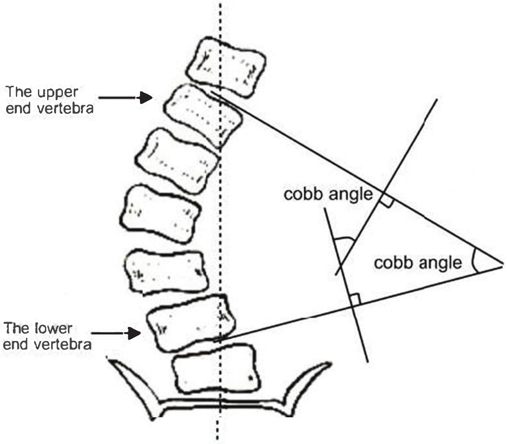
Figure 1. Definition of Cobb angle.
Applsci 13 03817 g001
Figure 2. The network structure for vertebral key points detection.
Applsci 13 03817 g002
Figure 3. Spine X-ray data set annotation (Left is vertebral center annotation and right is locating points annotation).
Applsci 13 03817 g003
Figure 4. Training Loss.
Applsci 13 03817 g004
Figure 5. Prediction results of vertebral center points and four anchor points.
Applsci 13 03817 g005
Figure 6. The result after filtering noisy points.
Applsci 13 03817 g006
Figure 7. Before and after correction.
Applsci 13 03817 g007
Table 1. Comparison of detection results of spinal key points.
Parameters (M)MAPE (%)FPS (Hz)
Hourglass193.629.788.43
HrNet242.6010.036.65
Proposed method13.469.2414.44
Table 2. Impact of positioning points and correction formula on Detection Results.
Locating PointsModifier FormulaMAPE PT (%)MAPE MT (%)MAPE TL (%)Accuracy of End Vertebrae Selection (%)
1 42.9635.6438.0320.6
2 26.7318.5821.0634.4
3 25.4533.1928.2778.1
415.3210.8711.3683.8
PT (proximal thoracic), MT (main thoracic), TL (thoracolumbar).
Table 3. Comparison of detection results of spinal key points.
ICC (95% CI)MAD ( )
Intra-observerObserver10.9512.24
Observer20.9582.16
Inter-observer1st0.9402.63
2nd0.9422.55
Table 4. Consistency analysis of Cobb Angle automatic measurement and manual method.
ICC (95% CI)MAD ( )
Observer1 & Auto0.8973.13
Observer2 & Auto0.9013.04
Disclaimer/Publisher’s Note: The statements, opinions and data contained in all publications are solely those of the individual author(s) and contributor(s) and not of MDPI and/or the editor(s). MDPI and/or the editor(s) disclaim responsibility for any injury to people or property resulting from any ideas, methods, instructions or products referred to in the content.