Abstract
Industrial defect detection plays an important role in smart manufacturing and is widely used in various scenarios such as smart inspection and product quality control. Currently, although utilizing a framework for knowledge distillation to identify industrial defects has achieved great progress, it is still a significant challenge task to extract better image features and prevent overfitting for student networks. In this study, a reverse knowledge distillation framework with two teachers is designed. First, for the teacher network, two teachers with different architectures are used to extract the diverse features of the images from multiple models. Second, considering the different contributions of channels and different teacher networks, the attention mechanism and iterative attention feature fusion idea are introduced. Finally, to prevent overfitting, the student network is designed with a network architecture that is inconsistent with the teacher network. Extensive experiments were conducted on Mvtec and BTAD datasets, which are industrial defect detection datasets. On the Mvtec dataset, the average accuracy values of image-level and pixel-level ROC achieved 99.43% and 97.87%, respectively. On the BTAD dataset, the average accuracy values of image-level and pixel-level ROC reached 94% and 98%, respectively. The performance on both datasets is significantly improved, demonstrating the effectiveness of our method.
1. Introduction
Industrial defect detection is one of the most important technologies to ensure the quality of products and maintain the stability of production, aiming at detecting defects in various industrial products. Recently, with the emergence of new technologies in the fields of computer vision and deep learning [1,2], vision-based industrial defect detection technology has been developed significantly. Industrial defect detection has become one of the important basic research and technology in intelligent manufacturing. It is widely used in unmanned quality inspection [3], intelligent inspection [4], video surveillance [5], etc. At present, the main difficulties and challenges of industrial defect detection lie in two aspects. One is the about data, such as the lack of abnormal samples, unpredictable defect patterns, more types of defects, and complex background of defect images. The other is that industrial vision defect detection requires methods with high accuracy, even to detect subtle defects.
Facing the difficulties and challenges in industrial defect detection, many approaches are currently available in the literature, which can be roughly categorized into three categories. The first category is currently designed for detection of synthetic abnormal samples, such as Cutpaste [6], and NSA [7]. The main purpose is to use the neural network to classify normal samples and synthetic abnormal samples for binary classification and then perform abnormality detection by the Gaussian probability density function. These methods require image pre-processing operations before model training, thus increasing the model complexity. Meanwhile, there is still a gap between the synthesized anomalous samples and the real ones. So, how to synthesize good anomaly samples is another challenge. The second category is based on the comparison at the pixel level of the image. The idea is to reconstruct a normal image that most closely resembles the input image, and then the difference between the reconstructed image and the input image is lie in the defective region. Such methods often use self-encoding models and generative models, including auto-encoder (AE) [8,9], generative adversarial networks (GAN) [10,11], etc. However, the pixels of the reconstructed image may not be aligned with the input image, and the reconstruction process may also change the style of the image, which can lead to detection errors and degrade the performance of the detection. In addition, the pixel level is more susceptible to noise interference, resulting in poor robustness of detection. In this regard, researchers turn to focus on feature space. Naturally, the third category is based on the feature similarity [12,13]. It is generally considered that the feature vectors of normal regions are more similar or closer, while the feature vectors of anomalous regions are different. The core objective of such methods is to find distinguishable feature embeddings and reduce the interference of irrelevant features. The features extracted by CNN contain information about the local perceptual field, instead of considering only individual pixels. Meanwhile, it does not require very strict spatial alignment, increasing the tolerance to noise interference. Some teacher-student network frameworks are proposed based on feature similarity [14,15]. The main idea is that the teacher network and the student network will produce different feature representations in the anomaly region since the training uses normal samples and the student network has not seen anomalous samples. Their framework has two main shortcomings. One is that they all use a single-teacher network, which may be deficient in extracting features, and the other is that the teacher and student networks use the same architecture, which may produce overfitting.
To address the issues of the teacher–student network, a new network architecture was designed. Firstly, for a single teacher network, the extracted features may be not representative enough. To overcome this, a two teacher network with inconsistent architectures is proposed to extract features for diverse feature learning. This can extract more information from the image and facilitate the detection of defective areas of the image. Secondly, the feature maps of the two teacher networks show numerous channels, but the relative importance of each channel varies. Meanwhile, the contribution of each teacher to the anomaly detection results is different. So, the attention mechanism is introduced to solve these issues. This allows the model to focus more on the important features and improves accuracy of the model. Finally, if the student network and the teacher network architectures are consistent, it may produce overfitting. It means that the student network is also able to reconstruct the anomaly region well, which can have a significant impact on our test results. The performance of the student network needs to be lower than the teacher network. So, a simple student network was redesigned to improve our AUC results, and its structure was not consistent with that of the teacher network.
The main contributions are summarized as follows:
- A teacher–student network architecture with two teachers is adopted for industrial image anomaly detection and localization, extracting features of images from multiple models.
- For each channel of the teacher network, the attention mechanism is employed. In addition, the iterative attention feature fusion method for the feature fusion of the two teachers is used. For the teacher and student networks, inconsistent architectures are used to mitigate overfitting.
- A large number of experiments were conducted on Mvtec and BTAD datasets to demonstrate the effectiveness of our approach.
The rest of this paper is organized as follows:
2. Related Work
Industrial defect anomaly detection and localization have been studied in recent years and a lot of literature has appeared. There are different divisions from different perspectives. We divide it into four components, image reconstruction and recovery, embedding-based, abnormal sample synthesis, and knowledge distillation.
2.1. Image Reconstruction and Recovery
The idea of image restoration methods is to assume that the parameters of the model are only trained from normal samples. The model can only reconstruct the normal samples well, while the defective areas of the abnormal samples will produce large reconstruction errors. Such methods include autoencoder (AE) [8,9], variational autoencoder (VAE) [16], and generative adversarial networks (GAN) [10,11]. However, the image reconstruction-based approach has the disadvantage that the model may still reconstruct the unseen defects completely. So, another popular approach was introduced to store normal features by introducing feature memory [17,18]. The researchers introduced memory to store the features of normal training samples, and in the inference phase, the sample features of the image to be tested are matched with the features in memory and reconstructed with them.
Image recovery methods treat defects as noise and consider it as a denoising process. The core idea of such methods is to add defects to a normal image and then train a network model to recover it to the corresponding original image. One of the core issues of such methods is how to design defective images for construction. For example, Ref. [19] superimposed Gaussian noise on the original image. Ref. [20] used attribute cancellation. Ref. [21] took into account the positional relationships in the image, borrowed from puzzle restoration [22] to disrupt the order of image blocks in the original image, and trained the network to restore them. Other methods are to overlay a mask on the original image and train the network to restore what is covered by the mask. Ref. [23] added random rectangular masks to normal samples to simulate real defects. Ref. [24] randomly selected superpixels of the image as a mask for training the model.
2.2. Embedding-Based
The purpose of feature similarity methods is to find feature embeddings that are distinguishable. It consists of deep one-class and feature distance metric methods. The deep one-class classification method [25] extracts the features of normal images through neural networks during training, and makes the extracted feature vectors of normal images as compact as possible, constructing a separation plane of normal feature boundaries in the feature space. During testing, the model extracts the features of the sample to be tested and maps them to the feature space. Then, it determines whether the test sample is abnormal according to the separation plane. Ref. [13] proposed the deep support vector data description (Deep SVDD) method, where the features of normal samples would be near a centroid. The centroid in Deep SVDD is replaced by a bias term in the neural network in FCDD [26]. FCDD directly locates the abnormal sites by the feature maps obtained from the fully convolutional network. Ref. [27] avoid the problem of model degradation by maintaining the semantic information of the features. Furthermore, Ref. [28] introduced multiscale to improve the detection capability. To improve the performance of one-class classification, self-supervised learning is another effective tool. The key to this approach is to design a self-supervised proxy task that facilitates defect detection by using normal samples to construct supervised information. Ref. [29] proposed a method based on RotNet [30], which applies a geometric transformation to the input data and trains a network that recognizes the transformation used. In addition, researchers have used self-supervised methods that create negative samples [6,31] to improve the discriminative power of classification models. Ref. [31] used images generated early in the training process.
The method of feature distance metric performs distance metric in feature space. Ref. [32] proposed SPADE based on the k-nearest neighbor (kNN) method, which first extracts the feature vectors of the training set using a CNN model pretrained on ImageNet [33] to build a database of normal samples. Then, it uses the kNN method to retrieve the k normal samples that are most semantically similar to the sample to be tested. The deep statistical model-based approach models the probability distribution of the features of the normal samples, eliminating the need to build a large normal sample database. Ref. [34] first extracted multiscale features of normal samples using a pre-training network and modeled each feature map as a multivariate Gaussian distribution. In the testing phase, the Marxian distance between the feature vector of the sample to be tested and the normal distribution is used to measure the presence of defects in the sample. Ref. [35] further modeled the multivariate Gaussian distribution on the image blocks, achieving pixel-level segmentation. Ref. [36] introduced the normalizing flow (NF) model to enhance flexibility.
2.3. Abnormal Sample Synthesis
Recently, many papers have used various methods to synthesize anomalous samples. The Cutpaste method [6] simulated anomalous samples by using a random patch from the image, and then the patch was pasted to any region of the image. In the object class, the patch may be pasted to the outside of the object, so Ref. [7] cut the patch from the surface of the object and pasted it to the object. Ref. [37] was to simulate various anomalies on images using data augmentation methods. Ref. [38] adopted two-dimensional Perlin noise to simulate the anomaly, but it was still a bit different from the actual anomaly.
2.4. Knowledge Distillation
The knowledge distillation network architecture consists of a pretrained teacher network and a trainable student network. In anomaly detection training, normal samples are used. If the input is a normal sample, the extracted features of the teacher network and the student network are closer together, and conversely, they are further apart. For example, US [14] used a teacher and multiple students to extract features of the samples. the US method utilized only the last layer of the network for distillation, while MKD [39] utilized multiple feature layers in the middle of the network for knowledge distillation. To improve the detection performance, Ref. [15] proposed an inverse distillation architecture, where the extracted features by the teacher are first compressed and then decoded by the student network. DeSTSeg [40] introduced the idea of segmentation into the knowledge distillation architecture, which also yields good results.
3. Methods
Given an input image, the task aims to detect anomalies while leveraging a reverse distillation framework, in which the student network imitates the behavior of the teacher network. The key is how to design a teacher and student network. Our framework is proposed in Figure 1. It consists of three modules: two different pretrained teacher encoders E, a multiple attentional feature fusion module, and a student decoder D. First, the two different pre-trained teachers extract multi-scale features in different layers and concatenate them separately. Second, we fuse features of the same layer and different branches using an attention mechanism and compress the obtained feature map into a low-dimensional feature vector. Finally, the student network decodes the low-dimensional feature vectors to obtain the feature maps, in which we can calculate the loss and generate multiscale similarity maps of each layer. In the testing stage, the anomaly map is generated by fusing these multiscale similarity maps.
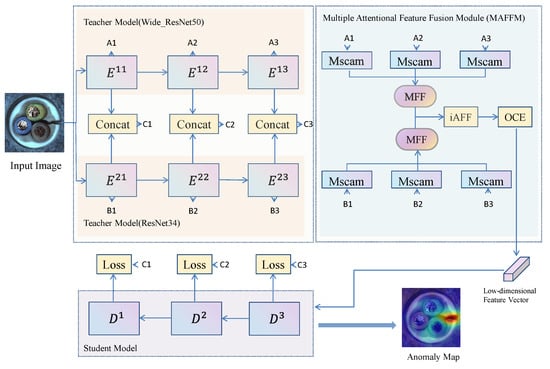
Figure 1.
Overview of our proposed framework for anomaly detection and localization. A contains A1, A2, and A3. Similarly, A2 and A3 are the same as A1. In the same way, B and C have the same properties as A. Our model consists of two different pretrained teachers encoder E, a multiple attentional feature fusion module, and a student decoder D. A multiscale channel attention module (Mscam) is used to fuse features in different layers from E and ensemble high-level and low-level features from Mscam by multiscale feature (MFF) block. Iterative attentional feature fusion (iAFF) is adopted to fuse features from two MFF and map it onto a compact feature vector by a one-class embedding (OCE) block. By minimizing the similarity loss between the two teacher models, student D learns to imitate the behavior of concatenated features in training. The anomaly map is generated by fusing the multiscale similarity maps of the student decoder.
3.1. Teacher Model
Currently, many distillation network architectures focus on distillation from a single teacher to a single student for anomaly detection and localization [15]. However, in the human learning process, a student does not learn from only one teacher; instead, he may learn from different teachers or different sources of information. Multiple teacher models provide multiple interpretations of the student model’s task by providing multiple streams of information, and the student model can use the teacher model’s views of the target task to improve the model’s performance. Thus, an ensemble of multiple teacher network predictions typically yields better performance than a single teacher network. Therefore, two teachers’ distillation networks are adopted.
Due to the different teachers needed, ResNet34 and Wide_ResNet50 pretrained on ImageNet are used in our framework [41,42]. They are enabled to extract rich features from images. In them, the last block (conv5_x) is removed and the output feature maps are extracted by the remaining blocks (conv2_x, conv3_x, and conv4_x). In Wide_ResNet50, they are named E11, E12, and E13, respectively. Similarly, they are known as E21, E22, and E23 in ResNet34, respectively. Finally, we fuse E11 and E21, E12 and E22, and E13 and 23, respectively, and then use them as intermediate feature layers of the network.
Since it has only one student decoding network for calculating the loss, it needs to fuse the two teachers’ feature channels and use a simple concatenation operation. For knowledge transfer, cosine similarity is used as our loss. The loss function is defined in Equation (1). In training, the size of the input image is 224 × 224 × 3, so the size of the first layer (E11, E21) feature map is 64 × 64 × 320, the second layer (E12, E22) feature map is 32 × 32 × 640, and the third layer (E13, E23) feature map is 16 × 16 × 1280. After fusion, the feature maps of each layer are 64 × 64 × 320, 32 × 32 × 640, and 16 × 16 × 1280, respectively.
In order to obtain a two-dimensional anomaly map , the formula is calculated as follows.
where and represent the feature vectors extracted from the teacher network and the student network, respectively. The h and w are defined as the height and width of the feature map, and k denotes the number of feature layers.
In the training process, the loss function L is represented as follows.
where h, w and k have the same meaning as in Equation (1).
3.2. Multiple Attentional Feature Fusion Module
On the one hand, every feature layer in a teacher network has many channels, but every channel is not equally important. On the other hand, for the learned features of a multiteacher network, it may not be the best operation to fuse them by simple add and concatenation operations. Therefore, the attention mechanism and iterative attention feature fusion are used to design a module.
A combination module named MAFFM is designed. It consists of the Mscam module, iAFF module, MFF module, and OCE module. Details of the modules can be found in the reference [15,43]. The Mscam module uses two branches with different scales to extract channel attention weights. One branch uses Global Avg Pooling to extract the attention of global features, and the other branch directly uses point-wise convolution to extract the channel attention of local features. Therefore, it is used in every layer of two teachers. In the Mscam network structure, there is a channel average distribution coefficient r, for which we made ablation experiments. After the Mscam, the feature map of every layer is still 64 × 64 × 320, 32 × 32 × 640, and 16 × 16 × 1280, respectively. The MFF module is a multiscale fusion module, which is to fuse feature maps of different sizes into the same size. Thus, it can get a feature map of size 16 × 16, and the channel number is 3072. The iAFF module uses an additional layer of attentional feature fusion(AFF) module to generate better initial features. After iAFF module, it can obtain a feature map of size 16 × 16 × 3072. The purpose of the OCE block is to project the high-dimensional feature vector into the low-dimensional space, using the residual connection block of ResNet. The design of the module can be found in the literature [15]. Finally, it can get a low-dimensional feature vector with a size of 8 × 8 × 2048.
3.3. Student Model
In some distillation architectures for anomaly detection, the same architecture is used in some literature for both teacher and student networks [15]. Since neural networks are generalizable, the student network may be able to reconstruct the anomaly region features well, leading to reduced performance of the detection. Therefore, it needs to design a more suitable network. In addition, in order to match the feature channels of the two teacher intermediate layers, a student decoding network is designed to decode the feature maps from the low-dimensional features. The student decoding network is shown in Figure 2.
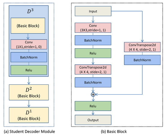
Figure 2.
Student decoder module and basic block in our student decoding network.
Motivated by the residual connection block in ResNet [41], we adopt it to fuse different scales of feature maps in the basic block (see Figure 2b). In the basic block, one branch is composed of a 4 × 4 deconvolution(ConvTranspose2d) layer and a BatchNorm layer, which aims to better preserve the original features. The other branch mainly consists of a 3 × 3 convolution and a 4 × 4 deconvolution(ConvTranspose2d). The 3 × 3 convolution is followed by a BatchNorm layer and a Relu layer, changing the input channels to match the number of output channels of the teacher network. The 4 × 4 deconvolution(ConvTranspose2d) is to change the size of the feature map to match the size of the feature map of the teacher network. Finally, the two branches are summed and outputted by the Relu activation layer.
The student decoder module(see Figure 2a) is the same as the teacher network. There are three layers in total, and it is an inverse structure. The D3 module consists of a basic block and a 1 × 1 convolutional layer, followed by a BatchNorm layer and a Relu layer. The purpose of the 1 × 1 convolution is mainly to change the input channel to match the output channel of the corresponding teacher network. The D2 and D1 modules are both composed of the basic block.
3.4. Training and Inference
In the training, the model uses all normal images and no abnormal images. The student network tries to mimic the output of the teacher network so that the features learned by both networks are as similar as possible for the same image. The loss function is to calculate the similarity of the feature maps of the corresponding layers. The main purpose of the training is to reduce the loss of function.
In the inference stage, both image-level anomaly score and pixel-level anomaly score are considered for anomaly detection and localization. When a normal image is input, the teacher network and the student network learn feature representations on a normal region with high similarity. On the contrary, when the image is abnormal, the pretrained teacher network can generate discriminative feature representations in both normal and anomalous regions, but the student network cannot, causing low similarity. In the student network, it needs to calculate a similarity value in each pixel. To be consistent with the image size, we will restore the feature map to the same size as the original image by bilinear up-sampling operation. Specific details can be found in the references [15]. Finally, it can get the pixel-level anomaly scores map by Gaussian filtering. In the image-level anomaly score, the maximum value is used in the pixel anomaly map as the sample-level score.
4. Experiments
To verify the effectiveness of our proposed method, the MVTec AD and BTAD datasets are used to evaluate our performance. Additionally, the ablation study is conducted on the MVTec dataset to examine the impact of various blocks or parameters on the results.
4.1. Datasets
MVTec AD is an industrial inspection-focused dataset for comparing anomaly detection methods. There are 15 different object and texture categories. Each class is split into a training set and a testing set. There are 3629 training images of typical objects and 1725 test images with various types of anomalies. For the test image, pixel-level binary annotations for anomalous images in the test set are provided.
BTAD is a dataset of actual industrial anomalies. The datasets include 2830 images of 3 industrial products that display flaws on their bodies and their surfaces. Additionally, it is separated into 1800 training images and 741 test images. It contains 3 categories, two objects, and one texture. The test datasets only contained one type of anomaly.
4.2. Evaluation Protocol
There are two evaluations, which are image-level evaluation and pixel-level evaluation. They both use the operating characteristic curve (ROC) and area under the curve (AUC) as the evaluation metric, called ROC-AUC. The ROC curve is a graph that shows the performance of a classification model across all thresholds. The two parameters that control this curve are the true positive rate (TPR) and the false positive rate (FPR). The equations are defined in (2) and (3).
The AUC calculates the area under the ROC curve in two dimensions between (0,0) and (1,1). The network reports the ROCAU scores after being trained separately for each object class.
For more accurate evaluation of anomaly localization performance, the per-region-overlap (PRO) metric is used. Unlike for pixel-by-pixel measurements, the PRO score treats anomalous regions of any size equally.
4.3. Implementation Details
The NVIDIA GTX Geforce 2070s GPU and the Ubuntu 18.04 operating system are used for the experiments. In experiments, the pre-trained Wide_ResNet50 and ResNet34 are used as our backbone in two teacher networks, and the student network is designed by ourselves. All the image input resolutions in MVTec and BTAD are set to 256 × 256. To train our model, Adam is used as the optimizer with parameter between 0.5 and 0.999. The learning rate uses the cosine annealing strategy, which the parameter period is 32. The initial value of the learning rate is 0.005. A total of 200 epochs are trained with a batch size of 4. For the student network, the Kaiming initialization method for network parameters is used. The random seed is set to 88. For additional details, it can refer to the open source code of the ADRD method.
4.4. Results
For comparisons with other work, we use the results mentioned in the original papers for compared methods. In image-level anomaly detection, we compare our model with the five kinds of existing models, including image restoration models, embedding-based models, abnormal sample synthesis models, flow-based models, and knowledge distillation models. The image restoration models contain AnoGAN [44], UniAD [45] and RIAD [46]. The embedding-based models consist of Psvdd [47] and PaDiM [35]. Abnormal sample synthesis models contain Cutpaste [6], NSA [7] and Draem [38]. Models for knowledge distillation involve US [14] and ADRD [15]. CFLOW-AD [48] is based on flow models. Our baseline is based on the ADRD model.
Table 1 shows the results of our image-level anomaly detection. From Table 1, it can see that our model outperformed other models in terms of the overall average value, achieving 99.43. In addition, from the perspective of texture and object class, the results of our method are also higher than other models, reaching 99.68 and 99.18, respectively. It shows that the knowledge distillation model is valuable in image anomaly detection.

Table 1.
Image-level anomaly detection results on MVTec AD dataset. Methods achieved for the top one ROC-AUC (%) are highlighted in bold. (Note: added reference numbers and 2 latest methods in table, one of which is SOTA method).
In addition, it’s obvious that our model gains further improvement compared with the ADRD baseline and outperforms other models. It demonstrates that the two teacher networks, the attention mechanism, and the inconsistent teacher–student network module have a positive effect. The US is similar to our method, but it does not use the inverse teacher–student network architecture, we believe that the student network may not be good at identifying anomalous regions in the inverse structure. Some categories have better results than ours, such as Grid, Capsule, and Pill. However, our results are almost the same as theirs.
For pixel-level anomaly detection, the comparison baselines include US [14], SPADE [32], PaDiM [35], Cutpaste [6], Draem [38], ADRD [15], NSA [7], CFLOW-AD [48] and UniAD [45]. Compared to the methods provided at the image-level anomaly detection, some models are not added to our table, and the data are not provided in the paper.
From Table 2, it can see that our method outperforms the other methods in pixel-level anomaly detection with 97.87, which proves that our method is effective. In the texture class and target class, it can see that the result of our method is the best in the target class, reaching 98.27, but the texture class is not. The Draem method process segments the simulated anomaly samples after simulating the anomaly samples. With this approach, it may have good results for pixel-level discrimination. But our method is directly comparing the similarity between regional feature vectors.
Table 2.
Pixel-level anomaly detection results on MVTec AD dataset. Methods achieved for the top one ROC-AUC (%) are highlighted in bold. (Note: added reference numbers and 2 latest methods in table, one of which is SOTA method).
In Table 3, we show the PRO scores of various methods in the Mvtec dataset. As can be seen from the table, we achieved the best result of 94.66. We only compared three methods since other literature did not provide PRO scores.
Table 3.
PRO scores of various methods on MVTec dataset.
We also contrast our model with a few others on the BTAD dataset, such as the autoencoder [50] and the VT-ADL method [49]. From Table 4, it can see that the performance of our method outperforms other models in image-level anomaly detection. Since the other methods do not give pixel-level anomaly detection scores, it can not compare them. Individually, the two categories 1 and 2 are better than our results in the AE + MSE + SSIM method, which mainly uses the autoencoder method. The MSE is the mean square error. The SSIM is the luminance, structure, and contrast of the image.
Table 4.
Image-level and Pixel-level anomaly detection results on the BTAD dataset. Methods achieved for the top one ROC-AUC (%) are highlighted in bold. “-” means that no pixel-level anomaly score is given in the method. (Note: added reference numbers).
Figure 3 shows the visualization results of our image anomaly detection. The red color indicates the region considered by the model to be a relatively high anomaly, the blue color indicates the region with a relatively low anomaly, and the green color region indicates the region with a slight anomaly. The first row represents the original image, the second row represents the mask image, and the third row is the visualization result. From Figure 3, it can see that the defective regions can be located, including the places where there are multiple anomalous regions. However, some areas are incorrectly localized. For example, most of the background areas of the screws and carpet show slight anomalies.
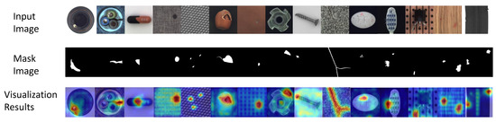
Figure 3.
Image anomaly detection visualization results. The first row represents the original image, the second row shows the mask image, and the third row is the visualization result.
In Figure 4, failure cases are shown. From our visualization results, we have selected a few samples where errors occurred. First, the background may affect the results of our model predictions in the object class. In the first and second columns of Figure 4, it can see that there is a little contamination in the background, marked with red colored boxes, and the visualization results show that there is a high level of outliers in these areas. Second, the area of the anomalous region is not fully localized. In the third column of Figure 4, it can see that the display of the anomalous area is incomplete and only a part of it is shown.
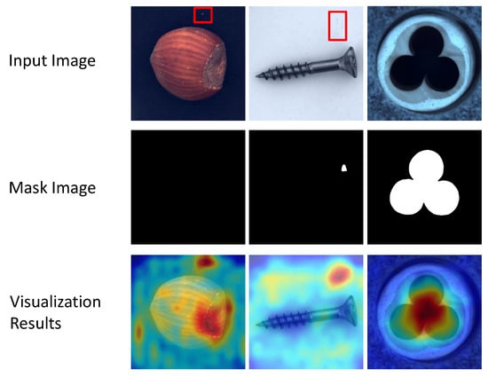
Figure 4.
The case of failure in our method. Several samples were selected from our test dataset, the top is the input image, the middle is the mask image, and the bottom is the visualization result.
In Figure 5, we did the statistics of the abnormal scores. Normal samples are shown in blue and abnormal samples are shown in yellow. As can be seen from Figure 5, the model is able to distinguish the normal samples from the abnormal samples well. However, some categories cannot be distinguished well and may require a better model or more training epochs.
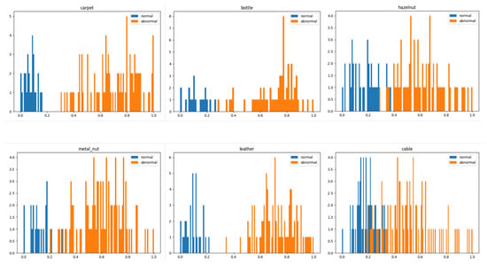
Figure 5.
Histogram of sample abnormal scores. Blue indicates normal samples and yellow indicates abnormal samples. The horizontal axis indicates the abnormal scores and the vertical axis indicates the counts.
4.5. Ablation Study
Teacher networks are important for feature extraction of images, and in Table 5, we verified the effect of using pretraining and nonpretraining networks on the image-level and pixel-level anomaly detection results. From Table 5, it can be seen that using pretraining can improve the results by about 20 points, indicating that using pretraining can extract the features of the image well.
Table 5.
Image-level and pixel-level anomaly detection results with teacher network using pretraining and nonpretraining.
In the attention mechanism module, we investigated the image feature channel division parameter r to see its effect on the anomaly detection results at the image-level and pixel-level, and the results are shown in Table 4. As can be seen from Table 6, the pixel-level results have a relatively small change in value as the r parameter changes. At the image-level anomaly detection results have some variation as the r parameter changes. It indicates that the division of image feature channels has some influence on the image-level anomaly detection results.
Table 6.
Image-level and pixel-level anomaly detection results for the attention mechanism module with channel division parameter r.
In Table 7, the baseline represents the adoption of the original network, including one teacher and student network. New Student Network represents the replacement of the original student network with a new student network, which is designed by ourselves. Two Teachers Network means replacing a single teacher network with two teacher networks. Mscam represents the addition of two teacher network feature channels to the attention mechanism module separately. Iaff represents the feature fusion of the two-teacher network feature channels again.
Table 7.
Ablation study of designed networks and modules for image-level and pixel-level anomaly detection results.
Both image-level and pixel-level anomaly detection results are improved by using different architectures for the teacher and student networks. This suggests that the powerful performance student network may cause overfitting and recover the anomalies as well.
Better feature representation can be extracted using two teacher networks. In Table 6, it can observe that the two teacher network achieves good results in image-level anomaly detection, but the pixel-level anomaly detection results are almost unchanged.
The use of an attention mechanism and feature fusion module enables better extraction of useful features. As can be seen from Table 6, the image-level and pixel-level anomaly detection results achieve a good result. The attention mechanism can extract better feature channels according to their importance, and the feature fusion module can assign higher weights to the teacher network that provides valuable features.
5. Conclusions
We propose to use reverse knowledge distillation with two teachers for industrial defect detection. In the teacher–student network, a two-teacher network with inconsistent architectures is employed to extract features for diverse feature learning. To focus on the important features and improves the accuracy of the model, an attention mechanism is adopted in the teacher network and an iterative attentional feature fusion is used for the feature fusion of the two teacher networks. In the student network, the student network is designed to prevent overfitting. Extensive experiments are conducted on Mvtec and BTAD datasets. From the results, both image-level and pixel-level anomaly scores are improved. However, the pixel-level performance improvement is not high, and it needs to be investigated in the future.
Author Contributions
Conceptualization, N.L. and M.P.; methodology, N.L. and H.S.; software, M.P.; validation, M.P.; formal analysis, N.L.; investigation, M.P.; resources, N.L.; data curation, M.P.; writing—original draft preparation, M.P.; writing—review and editing, N.L. and P.G.; visualization, M.P.; supervision, N.L.; project administration, N.L.; funding acquisition, N.L. All authors have read and agreed to the published version of the manuscript.
Funding
This research is supported in part by the Natural Science Foundation of Jiangsu Province of China (BK20222012), Guangxi Science and Technology Project (AB22080026/2021AB22167), National Natural Science Foundation of China (No. 61375021) and the Natural Science Key Project of Anhui Provincial Education Department (No. KJ2020A0636, No. KJ2021A0937, No. 2022AH051683, No. 2022AH051670, No. 2022AH051669).
Institutional Review Board Statement
Not applicable.
Informed Consent Statement
Not applicable.
Data Availability Statement
The data that support the findings of this study are available from the first author, Mingjing Pei, upon reasonable request.
Conflicts of Interest
The authors declare no conflict of interest.
References
- Chai, J.; Zeng, H.; Li, A.; Ngai, E.W. Deep learning in computer vision: A critical review of emerging techniques and application scenarios. Mach. Learn. Appl. 2021, 6, 100134. [Google Scholar] [CrossRef]
- Chen, Z.; Lu, Z.; Gao, H.; Zhang, Y.; Zhao, J.; Hong, D.; Zhang, B. Global to Local: A Hierarchical Detection Algorithm for Hyperspectral Image Target Detection. IEEE Trans. Geosci. Remote Sens. 2022, 60, 5544915. [Google Scholar] [CrossRef]
- Neubauer, K.; Bullard, E.; Blunt, R. Collection of Data with Unmanned Aerial Systems (UAS) for Bridge Inspection and Construction Inspection; Technical Report; Federal Highway Administration, Office of Infrastructure: Washington, DC, USA, 2021.
- Kuric, I.; Klarák, J.; Bulej, V.; Sága, M.; Kandera, M.; Hajdučík, A.; Tucki, K. Approach to Automated Visual Inspection of Objects Based on Artificial Intelligence. Appl. Sci. 2022, 12, 864. [Google Scholar] [CrossRef]
- Sharma, R.; Sungheetha, A. An efficient dimension reduction based fusion of CNN and SVM model for detection of abnormal incident in video surveillance. J. Soft Comput. Paradig. (JSCP) 2021, 3, 55–69. [Google Scholar] [CrossRef]
- Li, C.L.; Sohn, K.; Yoon, J.; Pfister, T. Cutpaste: Self-supervised learning for anomaly detection and localization. In Proceedings of the IEEE/CVF Conference on Computer Vision and Pattern Recognition, Online, 19–25 June 2021; pp. 9664–9674. [Google Scholar]
- Schlüter, H.M.; Tan, J.; Hou, B.; Kainz, B. Self-supervised out-of-distribution detection and localization with natural synthetic anomalies (nsa). arXiv 2021, arXiv:2109.15222. [Google Scholar]
- Gong, D.; Liu, L.; Le, V.; Saha, B.; Mansour, M.R.; Venkatesh, S.; Hengel, A.v.d. Memorizing normality to detect anomaly: Memory-augmented deep autoencoder for unsupervised anomaly detection. In Proceedings of the IEEE/CVF International Conference on Computer Vision, Seoul, Republic of Korea, 27 October–2 November 2019; pp. 1705–1714. [Google Scholar]
- Zhou, K.; Xiao, Y.; Yang, J.; Cheng, J.; Liu, W.; Luo, W.; Gu, Z.; Liu, J.; Gao, S. Encoding structure-texture relation with p-net for anomaly detection in retinal images. In Proceedings of the European Conference on Computer Vision, Glasgow, UK, 23–28 August 2020; pp. 360–377. [Google Scholar]
- Sabokrou, M.; Khalooei, M.; Fathy, M.; Adeli, E. Adversarially learned one-class classifier for novelty detection. In Proceedings of the IEEE/CVF International Conference on Computer Vision, Salt Lake City, UT, USA, 18–23 June 2018; pp. 3379–3388. [Google Scholar]
- Schlegl, T.; Seeböck, P.; Waldstein, S.M.; Langs, G.; Schmidt-Erfurth, U. f-AnoGAN: Fast unsupervised anomaly detection with generative adversarial networks. Med. Image Anal. 2019, 54, 30–44. [Google Scholar] [CrossRef]
- Wang, S.; Wu, L.; Cui, L.; Shen, Y. Glancing at the patch: Anomaly localization with global and local feature comparison. In Proceedings of the IEEE/CVF Conference on Computer Vision and Pattern Recognition, Online, 19–25 June 2021; pp. 254–263. [Google Scholar]
- Ruff, L.; Vandermeulen, R.; Goernitz, N.; Deecke, L.; Siddiqui, S.A.; Binder, A.; Müller, E.; Kloft, M. Deep one-class classification. In Proceedings of the International Conference on Machine Learning, PMLR, Stockholm Sweden, 10–15 July 2018; pp. 4393–4402. [Google Scholar]
- Wang, G.; Han, S.; Ding, E.; Huang, D. Student-teacher feature pyramid matching for unsupervised anomaly detection. arXiv 2021, arXiv:2103.04257. [Google Scholar]
- Deng, H.; Li, X. Anomaly Detection via Reverse Distillation from One-Class Embedding. In Proceedings of the IEEE/CVF Conference on Computer Vision and Pattern Recognition, Seattle, WA, USA, 19–20 June 2022; pp. 9737–9746. [Google Scholar]
- Zhi-Han, Y. Training Latent Variable Models with Auto-encoding Variational Bayes: A Tutorial. arXiv 2022, arXiv:2208.07818. [Google Scholar]
- Hou, J.; Zhang, Y.; Zhong, Q.; Xie, D.; Pu, S.; Zhou, H. Divide-and-assemble: Learning block-wise memory for unsupervised anomaly detection. In Proceedings of the IEEE/CVF International Conference on Computer Vision, Online, 11–17 October 2021; pp. 8791–8800. [Google Scholar]
- Park, H.; Noh, J.; Ham, B. Learning memory-guided normality for anomaly detection. In Proceedings of the IEEE/CVF Conference on Computer Vision and Pattern Recognition, Seattle, WA, USA, 13–19 June 2020; pp. 14372–14381. [Google Scholar]
- Zhang, X.; Mu, J. Deep anomaly detection with self-supervised learning and adversarial training. Pattern Recognit. 2022, 121, 108234. [Google Scholar] [CrossRef]
- Ye, F.; Huang, C.; Cao, J.; Li, M.; Zhang, Y.; Lu, C. Attribute restoration framework for anomaly detection. IEEE Trans. Multimed. 2020, 24, 116–127. [Google Scholar] [CrossRef]
- Salehi, M.; Eftekhar, A.; Sadjadi, N.; Rohban, M.H.; Rabiee, H.R. Puzzle-ae: Novelty detection in images through solving puzzles. arXiv 2020, arXiv:2008.12959. [Google Scholar]
- Noroozi, M.; Favaro, P. Unsupervised learning of visual representations by solving jigsaw puzzles. In Proceedings of the European Conference on Computer Vision, Amsterdam, The Netherlands, 11–14 October 2016; pp. 69–84. [Google Scholar]
- Haselmann, M.; Gruber, D.P.; Tabatabai, P. Anomaly detection using deep learning based image completion. In Proceedings of the 2018 17th IEEE International Conference on Machine Learning and Applications (ICMLA), Orlando, FL, USA, 17–20 December 2018; pp. 1237–1242. [Google Scholar]
- Li, Z.; Li, N.; Jiang, K.; Ma, Z.; Wei, X.; Hong, X.; Gong, Y. Superpixel masking and inpainting for self-supervised anomaly detection. In Proceedings of the BMVC, Online, 7–10 September 2020. [Google Scholar]
- Sohn, K.; Li, C.L.; Yoon, J.; Jin, M.; Pfister, T. Learning and evaluating representations for deep one-class classification. arXiv 2020, arXiv:2011.02578. [Google Scholar]
- Liznerski, P.; Ruff, L.; Vandermeulen, R.A.; Franks, B.J.; Kloft, M.; Müller, K.R. Explainable deep one-class classification. arXiv 2020, arXiv:2007.01760. [Google Scholar]
- Wu, P.; Liu, J.; Shen, F. A deep one-class neural network for anomalous event detection in complex scenes. IEEE Trans. Neural Netw. Learn. Syst. 2019, 31, 2609–2622. [Google Scholar] [CrossRef]
- Massoli, F.V.; Falchi, F.; Kantarci, A.; Akti, Ş.; Ekenel, H.K.; Amato, G. MOCCA: Multilayer One-Class Classification for Anomaly Detection. IEEE Trans. Neural Net. Learn. Syst. 2021, 33, 2313–2323. [Google Scholar] [CrossRef]
- Golan, I.; El-Yaniv, R. Deep anomaly detection using geometric transformations. Adv. Neural Inf. Process. Syst. 2018, 31. [Google Scholar]
- Komodakis, N.; Gidaris, S. Unsupervised representation learning by predicting image rotations. In Proceedings of the International Conference on Learning Representations (ICLR), Vancouver, BC, Canada, 30 April–3 May 2018. [Google Scholar]
- Pourreza, M.; Mohammadi, B.; Khaki, M.; Bouindour, S.; Snoussi, H.; Sabokrou, M. G2D: Generate to detect anomaly. In Proceedings of the IEEE/CVF Winter Conference on Applications of Computer Vision, Online, 5–9 January 2021; pp. 2003–2012. [Google Scholar]
- Cohen, N.; Hoshen, Y. Sub-image anomaly detection with deep pyramid correspondences. arXiv 2020, arXiv:2005.02357. [Google Scholar]
- Krizhevsky, A.; Sutskever, I.; Hinton, G.E. Imagenet classification with deep convolutional neural networks. Commun. ACM 2017, 60, 84–90. [Google Scholar] [CrossRef]
- Rippel, O.; Mertens, P.; Merhof, D. Modeling the distribution of normal data in pre-trained deep features for anomaly detection. In Proceedings of the 2020 25th International Conference on Pattern Recognition (ICPR), Milan, Italy, 10–15 January 2021; pp. 6726–6733. [Google Scholar]
- Defard, T.; Setkov, A.; Loesch, A.; Audigier, R. Padim: A patch distribution modeling framework for anomaly detection and localization. In Proceedings of the International Conference on Pattern Recognition, Online, 10–15 January 2021; pp. 475–489. [Google Scholar]
- Rudolph, M.; Wandt, B.; Rosenhahn, B. Same same but differnet: Semi-supervised defect detection with normalizing flows. In Proceedings of the IEEE/CVF Winter Conference on Applications of Computer Vision, Waikoloa, HI, USA, 3–8 January 2021; pp. 1907–1916. [Google Scholar]
- Yoa, S.; Lee, S.; Kim, C.; Kim, H.J. Self-supervised learning for anomaly detection with dynamic local augmentation. IEEE Access 2021, 9, 147201–147211. [Google Scholar] [CrossRef]
- Zavrtanik, V.; Kristan, M.; Skočaj, D. Draem-a discriminatively trained reconstruction embedding for surface anomaly detection. In Proceedings of the IEEE/CVF International Conference on Computer Vision, Online, 11–17 October 2021; pp. 8330–8339. [Google Scholar]
- Salehi, M.; Sadjadi, N.; Baselizadeh, S.; Rohban, M.H.; Rabiee, H.R. Multiresolution knowledge distillation for anomaly detection. In Proceedings of the IEEE/CVF Conference on Computer Vision and Pattern Recognition, Online, 19–25 June 2021; pp. 14902–14912. [Google Scholar]
- Zhang, X.; Li, S.; Li, X.; Huang, P.; Shan, J.; Chen, T. DeSTSeg: Segmentation Guided Denoising Student-Teacher for Anomaly Detection. arXiv 2022, arXiv:2211.11317. [Google Scholar]
- He, K.; Zhang, X.; Ren, S.; Sun, J. Deep residual learning for image recognition. In Proceedings of the IEEE Conference on Computer Vision and Pattern Recognition, Las Vegas, NV, USA, 26 June–1 July 2016; pp. 770–778. [Google Scholar]
- Zagoruyko, S.; Komodakis, N. Wide residual networks. In Proceedings of the British Machine Vision Conference (BMVC), York, UK, 19–22 September 2016. [Google Scholar]
- Dai, Y.; Gieseke, F.; Oehmcke, S.; Wu, Y.; Barnard, K. Attentional feature fusion. In Proceedings of the IEEE/CVF Winter Conference on Applications of Computer Vision, Waikola, HI, USA, 5–9 January 2021; pp. 3560–3569. [Google Scholar]
- Deecke, L.; Vandermeulen, R.; Ruff, L.; Mandt, S.; Kloft, M. Image anomaly detection with generative adversarial networks. In Proceedings of the Joint European Conference on Machine Learning and Knowledge Discovery in Databases, Wurzburg, Germany, 16–20 September 2019; pp. 3–17. [Google Scholar]
- You, Z.; Cui, L.; Shen, Y.; Yang, K.; Lu, X.; Zheng, Y.; Le, X. A unified model for multi-class anomaly detection. In Proceedings of the Neural Information Processing Systems, New Orleans, LA, USA, 2–4 December 2022. [Google Scholar]
- Zavrtanik, V.; Kristan, M.; Skočaj, D. Reconstruction by inpainting for visual anomaly detection. Pattern Recognit. 2021, 112, 107706. [Google Scholar] [CrossRef]
- Yi, J.; Yoon, S. Patch Svdd: Patch-Level Svdd for Anomaly Detection and Segmentation. In Lecture Notes in Computer Science; Springer: Berlin/Heidelberg, Germany, 2020; pp. 375–390. [Google Scholar]
- Gudovskiy, D.; Ishizaka, S.; Kozuka, K. Cflow-ad: Real-time unsupervised anomaly detection with localization via conditional normalizing flows. In Proceedings of the IEEE/CVF Winter Conference on Applications of Computer Vision (WACV), Waikoloa, HI, USA, 3–8 January 2022; pp. 98–107. [Google Scholar]
- Mishra, P.; Verk, R.; Fornasier, D.; Piciarelli, C.; Foresti, G.L. VT-ADL: A vision transformer network for image anomaly detection and localization. In Proceedings of the 2021 IEEE 30th International Symposium on Industrial Electronics (ISIE), Kyoto, Japan, 20–23 June 2021; pp. 1–6. [Google Scholar]
- Guo, X.; Liu, X.; Zhu, E.; Yin, J. Deep clustering with convolutional autoencoders. In Proceedings of the International Conference on Neural Information Processing, Guangzhou, China, 14–18 November 2017; pp. 373–382. [Google Scholar]


Disclaimer/Publisher’s Note: The statements, opinions and data contained in all publications are solely those of the individual author(s) and contributor(s) and not of MDPI and/or the editor(s). MDPI and/or the editor(s) disclaim responsibility for any injury to people or property resulting from any ideas, methods, instructions or products referred to in the content. |
© 2023 by the authors. Licensee MDPI, Basel, Switzerland. This article is an open access article distributed under the terms and conditions of the Creative Commons Attribution (CC BY) license (https://creativecommons.org/licenses/by/4.0/).