Lenke Classification of Scoliosis Based on Segmentation Network and Adaptive Shape Descriptor

Abstract

Scoliosis is a common spinal deformity that seriously affects patients’ physical and mental health. An accurate Lenke classification is greatly significant for evaluating and treating scoliosis. Currently, the clinical diagnosis mainly relies on manual measurement; however, using computer vision assists with an intelligent diagnosis. Due to the complex rules of Lenke classification and the characteristics of medical imaging, the fully automated Lenke classification of scoliosis remains a considerable challenge. Herein, a novel Lenke classification method for scoliosis using X-rays based on segmentation networks and adaptive shape descriptors is proposed. Three aspects of our method should be noted in comparison with the previous approaches. We used Unet++ to segment the vertebrae and designed a post-processing operation to improve the segmentation effect. Then, we proposed a new shape descriptor to extract the shape features for segmented vertebrae in greater detail. Finally, we proposed a new Lenke classification framework for scoliosis that contains two schemes based on Cobb angle measurement and shape classification, respectively. After rigorous experimental evaluations on a public dataset, our method achieved the best performance and outperformed other sophisticated approaches.

1. Introduction

Scoliosis is a spinal deformity where one or more spinal segments deviate from the center line of the body and curve laterally; it can also be accompanied by spinal rotation [1]. Scoliosis can occur in any age group, especially during adolescence, which is known as adolescent idiopathic scoliosis (AIS). The worldwide prevalence of AIS is approximately 0.5–5.2%, causing it to be the most common spinal deformity in adolescents [2]. Scoliosis not only changes in the spine’s shape and function, but can, in severe cases, lead to a range of diseases, such as nerve damage, arrhythmia, cardiopulmonary dysfunction, pulmonary failure, and even paralysis.

Whole spine X-rays are the most common imaging examination for diagnosing, treating, and prognosis of scoliosis. Evaluating the Cobb angle (a type of measurement of the lateral curvature of the spine), vertebral rotation, and other parameters in X-rays can effectively reflect scoliosis severity and provide a basis for establishing the best treatment plan [3]. Lenke et al. [4] proposed a new classification system for assessing scoliosis severity, which is known as the Lenke classification criteria, and this has since been the standard guideline for evaluating scoliosis in clinical practice. As shown in Figure 1, the Lenke classification criteria divide scoliosis into six types, from Lenke type 1 to type 6. Obtaining an accurate Lenke classification of scoliosis is integral for selecting the treatment modality, especially the surgical strategy.

The key steps for the Lenke classification of scoliosis include determining the location of each vertebra, computing the Cobb angle, and extracting the characteristic of the curve. In traditional methods, the key anatomical features of the spine are located and manually measured on the X-ray image using a ruler, protractor, and marker; then, using the Lenke classification criteria, the Lenke type is further determined by professional radiologists. However, manual measurement has many disadvantages, such as being time-consuming and having a large amount of errors, strong subjectivity, and high reliance on physician experience.

With the rapid development of artificial intelligence, computer vision application provides a more efficient way of diagnosing spinal diseases. Based on a comprehensive literature survey, three key visual techniques were identified as being involved in the Lenke classification of scoliosis.

The first is segmenting the spine image, that is, segmenting each vertebra from the spine image. Unet [5] is a remarkable deep learning model that employs an “encoder–decoder” architecture based on fully convolutional networks (FCN) [6]. Since then, numerous variants of Unet, such as UNet++ [7], MAnet [8], RMS-Unet [9], X-Net [10], and MQANet [11], have been developed for use in medical image segmentation and other scenarios. Many researchers have also attempted to improve Unet for spinal image segmentation [12]. For example, Sunetra et al. [13] proposed an SIUNet with an improvised inception block and new dense skip pathways, which achieved promising performance in spine image segmentation. Christian et al. [14] developed a coarse-to-fine approach for vertebrae localization and segmentation in CT images based on Unet, which achieved the best results in the MICCAI 2019 Vertebrae Segmentation Challenge [15]. Recently, another deep learning method, transformers and their variants, has gained great attention and achieved significant success in image segmentation [16]. Segmenter [17] is a superior transformer model for segmentation that is built on top of the recent vision transformer [18], which achieved state of the art in two scene image datasets. Recently, Rong et al. [19] proposed a new transformer for labeling and segmenting of 3D vertebrae for arbitrary field-of-view CT images, thus demonstrating the great potential of transformer methods in spine image segmentation.

The second is Cobb angle measurement or spinal curvature estimation with geometric calculation, which is generally based on the segmentation results [20]. Cheng et al. [21] proposed a novel method to compute the Cobb angles monitoring the connection relationships among the segmented vertebrae in the X-ray images. Yi et al. [22] proposed a spinal curvature estimation method built on top of the segmentation model. Kang et al. [23] developed a spine curve assessment method by using a confidence map and vertebral tilt field, which also provided local and global spine structural information. Although these methods provide an excellent means to automatically compute the Cobb angle, there is still room for improvement as they heavily rely on the segmentation results. However, accurately segmenting vertebra is extremely difficult owing to the unclear vertebral boundary in the X-ray images. In addition, these methods are difficult to directly apply to the Lenke classification of scoliosis, as they have high requirements for the Cobb angle accuracy and need more additional features.

The third is feature representation for spinal images, which are beneficial for evaluating scoliosis severity. These features include the shape, texture, spatial relationship, and others. For example, Bayat et al. [24] proposed a label method for the cervical, thoracic, and lumbar vertebrae using both texture and inter vertebral spatial information. Zhi et al. [25] proposed to describe the spine using curve fitting, with the parameters of the fitted curve used for shape classification.

Recently, some work has focused on the classifying scoliosis using the above visual techniques. For example, Yang et al. [26] proposed a classification scheme of mild AIS by using the bending asymmetry index (BAI) based on 3D ultrasound imaging. In [27], another Lenke classification system based on BAI and cobb angle measurement was designed and achieved promising performance in X-ray images. However, in the above method, the BAI calculations were semi-automatic and relied on manual annotation. Gardner et al. [28] proposed an effective method for the cluster analysis of Lenke types based on spinal and torso shape representation, but only Lenke type 1 was involved in this study. Rothstock et al. [29] designed a semi-automatic classification framework for 3D surface trunk data by analyzing the asymmetry distance of the complete trunk as a predictor for scoliosis severity. Zhang et al. [30] proposed a computerized Lenke classification approach based on Cobb angle measurement, which required the user to click the mouse to locate the vertebrae. To sum up, although various approaches have been proposed for classifying scoliosis with spine images, these methods still face many problems. First, most methods mainly provide some characteristics of the scoliosis as the output, such as the Cobb angle and most tilted vertebra [31,32]. Some recent work has focused on complete classification systems, but most are semi-automatic or rely on three-dimensional data; a fully automatic Lenke classification system with only X-ray images is rarely reported. In addition, the accuracy of Lenke classification greatly depends on the segmentation performance, and the design and selection of segmentation networks is challenging. Finally, the visual feature representation of scoliosis is another issue that must be carefully considered, as scoliosis has visually similar shapes and is difficult to distinguish in X-ray images. Therefore, it would be necessary to develop a complete automatic Lenke classification system that provides an accurate and efficient Lenke diagnosis in a visually interpretable manner.

To this end, we propose an automatic Lenke classification algorithm for scoliosis based on a segmentation network and an adaptive shape descriptor. Specifically, four important steps should be noted. First, a deep network based on Unet++ is employed to segment each vertebra in the spine X-ray images, and a post-processing approach is further used to enhance the segmentation effect. Thereafter, an automatic measurement system of the Cobb angle is designed, and then, an alternative Lenke classification solution for scoliosis is obtained. In addition, we propose an adaptive shape descriptor for segmented spine images to capture the discriminating shape features. Finally, a new Lenke classification algorithm for scoliosis is proposed by using the shape description and a KNN classifier. Performing rigorous experimental evaluations on a public dataset demonstrated that the proposed method achieved an accurate and robust performance for the Lenke classification of scoliosis. In summary, our contributions are fourfold:

(1)

A novel clinician-friendly automatic Lenke classification framework for scoliosis based on a segmentation network and shape feature description is proposed.

(2)

A new shape descriptor will be designed for segmented vertebrae, which can effectively describe the microscopic shape distribution of the vertebrae and adaptively adjust the matching weights.

(3)

A simple and efficient post-processing approach for spinal image segmentation is proposed to avoid segmentation errors.

(4)

A comprehensive evaluation will be performed for scoliosis, such as evaluating the impact of segmentation networks on Lenke classification and comparing of the Lenke classification frameworks based on the Cobb angle measurement and shape feature extraction, respectively.

The remainder of this paper is structured as follows: Section 2 describes the proposed Lenke classification method of scoliosis and the implementation detail, Section 3 presents the experimental evaluation and results, and Section 4 presents the conclusion and future perspectives.

2. Methods

In this section, we present the proposed method in detail. Section 2.1 introduces our overall research framework for the Lenke classification of scoliosis, and Section 2.2 presents the spinal image segmentation. In Section 2.3 and Section 2.4, we introduce an automatic measurement of the Cobb angle and describe the proposed shape descriptor. Finally, we introduce the Lenke classification algorithms of scoliosis in Section 2.5.

2.1. The Overall Framework for Lenke Classification of Scoliosis

In this section, we propose an overall framework for the Lenke classification of scoliosis, which can mainly be divided into four parts as shown in Figure 2.

First, we used deep neural networks to segment each vertebra from the spinal X-ray images. In practice, original spinal X-rays have complex imaging characteristics and are difficult to directly use for automatic Cobb angle measurement and Lenke classification. The segmentation networks can help with this process, providing the basis for the auxiliary diagnosis. Specifically, Unet++ [7] was selected for this purpose based on a comprehensive evaluation, and a novel post-processing strategy was proposed to improve the segmentation performance. Subsequently, an automatic Cobb angle measurement algorithm was designed, which can effectively recognize the vertebrae with maximum scoliotic tilt based on the segmented spinal image. Third, we proposed an adaptive shape descriptor to describe the spine’s overall and local curvature, in which four shape representation and matching strategies are fused to capture the discriminative features. Finally, two alternative methods to achieve the Lenke classification of scoliosis are proposed, i.e., using inference rules based on Cobb angles and using shape features based on the K-nearest neighbor (KNN) classifier [33]. In the following sections, each part of the proposed method will be elaborated.

2.2. Segmentation of Vertebrae

2.2.1. Segmentation Networks

In this section, we introduce Unet and Unet++ as the backbone segmentation networks.

As shown in Figure 3a, the basic Unet architecture consists of two parts: the convolutional encoder and decoder. The encoder part has a classical convolutional network architecture in which the ReLU activation function and 2 × 2 max pooling operations are performed for downsampling. Downsampling is beneficial for networks to improve their robustness to deal with image translation and rotation. In the decoder part, the deconvolution operations are performed to upsample the feature maps. More specifically, through the 3 × 3 deconvolution in two layers with the ReLU activation function, the final layer is computed using the convolution of 1 × 1 to obtain the segmentation results. Upsampling can retain the profile features and decode them to the original image’s size, and the skip connection between the encoder and decoder prompts Unet to preserve the full context of the input images. This particular connection pattern provides U-net with an edge in medical image segmentation. Unet++ is an improved Unet model that combines long and short connections. As shown in Figure 3b, the Unet++ architecture consists of an encoder and a decoder connected with nested dense convolutional blocks. Unet++ redesigns the skip connections and provides the flexible feature fusion in the decoders. In addition, the deep supervision process of Unet++ can achieve a significant speedup with only a modest drop in performance. Two key technical details of Unet++ are introduced as follows.

Connected domain. Suppose $x^{i,j}$ denotes the output of the node ${\mathit{X}}^{i,j}$, where i represents the down-sampling layer along the encoder, while j represents the convolution layer of the dense block along the skip connection. Then, the feature maps denoted by $x^{i,j}$ are calculated as follows:

$$x^{i,j}={\{}_{\Phi (\left[{[x^{i,k}]}_{k=0}^{j-1}, U(x^{i+1,j-1})\right],\hspace{1em}j>0}^{\Phi (D(x^{i-1,j})),\hspace{1em}\hspace{1em}\hspace{1em}\hspace{1em}\hspace{1em}\hspace{0.33em}\hspace{0.33em}\hspace{0.33em}\hspace{0.33em}\hspace{0.33em}j=0}\hspace{0.33em}$$

(1)

where function $\Phi (\cdot )$ is a combination of the convolution layer and an activation function, $D(\cdot )$ and $U(\cdot )$ represent a downsampling layer and an up-sampling layer, respectively, and [] indicates the concatenation layer. In the Unet++ architecture, if level j = 0, the nodes only receive one input from the previous layer of the encoder; if level j = 1, the nodes receive two inputs from two consecutive levels of the encoder sub-network; if level j > 1, the nodes receive j + 1 inputs, including j inputs from the previous same skip connection, and one input from the lower skip connection.

(2)

Segmentation loss. The hybrid loss combined binary cross-entropy with a dice coefficient is employed as follows:

$$\Gamma (Y,\stackrel{⌢}{Y})=-\frac{1}{N}{\displaystyle \sum _{b=1}^N(\frac{1}{2}\cdot Y_b\cdot \log {\stackrel{⌢}{Y}}_b+\frac{2\cdot Y_b\cdot {\stackrel{⌢}{Y}}_b}{Y_b+{\stackrel{⌢}{Y}}_b})}$$

(2)

where ${\stackrel{⌢}{Y}}_b$ and $Y_b$ denote the flatten predicted probabilities and the flatten ground truths of the $b^{th}$ image, respectively, and N is the batch size.

The proposed Lenke classification framework of scoliosis can be applied to more segmentation networks, such as transformer-based models. We will perform a comprehensive evaluation for different segmentation methods in the later experiments.

2.2.2. Automatic Post-Processing for Segmentation

Vertebrae tend to have low contrast in X-ray images, which may cause segmentation errors with deep networks, such as adhesion and speckle. These errors will further affect the Lenke classification performance. Therefore, we propose a simple post-processing approach to reduce this segmentation error by using adaptive geometric calculation; the computational flow is shown in Figure 4. Specifically, suppose $I_1=I_b\cup I_f$ is the segmented spine X-ray image created by segmentation networks, where I_b and I_f denote the back- and foreground regions, respectively, then the post-processing can be divided into four steps.

Step 1: performing the opening operation, i.e., erosion followed by dilation, for I_b and I_f, respectively. Then, I₂ can be obtained as follows.

$$I_2=((I_b\ominus B_b)\oplus B_b)\cup ((I_f\ominus B_f)\oplus B_f{)}_{ }$$

(3)

where ⊖ and ⊕ denote the dilation and erosion operation, respectively; B_b and B_f denote the convolution kernels. With this operation, some simple segmentation errors can be effectively eliminated, such as holes in the foreground and speckles in the background.

Step 2: identifying the adhesive vertebrae and impurity vertebrae. Specifically, traversing each vertebra from top to bottom, starting from the second vertebra, if the current vertebra is C₁ times larger than the previous one, then it is identified as an adhesive vertebra; if the current vertebra is C₂ times less than the previous one, it can be considered as an impurity vertebra. In case the first vertebra is abnormal, we repeat it again in the same manner from bottom to top. During the processing, the adhesive vertebrae are separately extracted as I₃, and the remaining vertebrae are marked as I₄. Any impurity vertebrae in I₄ are directly removed, and the output result is denoted as I₅. Based on the analysis of the segmentation effect, C₁ and C₂ were set as 1.8 and 0.5, respectively, in our experiments.

Step 3: segmenting the adhesive vertebrae, i.e., I₃. We first traverse the left and right boundaries of the adhesion vertebrae and search the left and right inflection points. If both can be determined, then the two inflection points are connected as the segmenting line of the two vertebrae; if one of them cannot be identified, then a parallel line is drawn as the segmenting line through the only inflection point. This parallel line is the intermediate result relative to the upper and lower boundaries of the adhesion vertebrae. If there is no obvious inflection point, then the entire adhesion vertebrae are equally segmented according to the size compared to its neighbors. In fact, in the experiments, we found that obvious inflection points can be searched in the most original segmentation results by using deep networks. The output of this step is denoted as I₆.

Step 4. the final post-processing result can be obtained by combining I₅ and I₆ as shown in Figure 4.

In fact, the post-processing is proposed in an unsupervised manner, which is simply calculated and can be used to alleviate the influence of segmentation error on the Lenke classification of scoliosis.

2.3. Automatic Measurement of Cobb Angle

The Cobb angle as an objective measure is used to quantify spinal curvature and is important for the Lenke classification system. The Cobb angle is traditionally measured manually by doctors on X-ray images using a pencil and protractor based on their experience. This type of traditional measurement could lead to some errors, and its inter- and intra-observer variability is high. Moreover, the accuracy and consistency of the Cobb angle measurement will affect the Lenk classification results and have significant implications for treating and managing of patients. Therefore, in this section, an automatic and effective Cobb angle measurement approach based on the segmented spinal block is proposed, as explained in the next paragraph.

The key links for measuring the Cobb angle based on computer vision are to identify the superior and inferior endplates of each spinal block. As shown in Figure 5, the Cobb angle automatic measurement framework consists of four steps. First, each vertebra can be segmented and locally separated by segmentation and using the post-processing algorithm. Second, a canny operator [34] is employed to detect edge of the spinal block, which is almost closed. Then, we traverse the upper and lower edges, respectively, and the sample points at regular intervals and at the same time. These sample points on the upper and lower edges are marked as green and yellow, respectively. As the segmented boundaries of each vertebra have a slight bend, some noise points may exist that could affect the fitting results. Therefore, a simple and effective strategy is employed to eliminate the noise and optimize the distribution of the simple points. Mathematically, suppose (a₀, a₁, …, a_n−1) are sampled n points, then we define the k-neighbors angle ${\overline{\theta }}_i$ for each point a_i, according to Formula (4), where we describe the average fluctuation degree of a_i. Subsequently, the average angle $\overline{\theta }$ of k-neighbors for the sequence of points can be obtained from Formula (5). To better explain these two formulas, we use Figure 5 as an example that has nine sampled points marked as (a₀, a₁, …, a₉). If k is set as 2, then each point forms two angles with its left and right neighbor points in turn. Specifically, for a₃, $\overrightarrow{a_3{a}_2}$ and $\overrightarrow{a_3{a}_4}$ form an angle denoted as ${\theta }_3^1$, $\overrightarrow{a_3{a}_1}$ and $\overrightarrow{a_3{a}_5}$ form an angle denoted as ${\theta }_3^2$. Then, the average fluctuation angle ${\overline{\theta }}_3$ of a₃ can be obtained by averaging ${\theta }_3^1$ and ${\theta }_3^2$. The average fluctuation angle of each point a_i can be calculated in a similar way. Subsequently, the average fluctuation angle of the point series (a₀, a₁, …, a₉) can also be obtained by taking the average.

Then, if point a_i satisfies $(\overline{\theta }-{\overline{\theta }}_i+\pi )\mathrm{mod}\pi >\delta$, then a_i is marked as noise points and will be further eliminated, where $\delta$ is a threshold that reflects the noise factor. As shown in Figure 5, the point marked as red is the noise point because its average fluctuation angle is quite different from that of other points. Through the preliminary experiment, we found that the noise points are mainly caused by the speckle error of the segmentation model, and there is a large deviation from the real boundary. Therefore, we set k and $\delta$ to 3 and $\pi /6$, respectively. After the optimized simple points have been obtained, the straight line representing the superior and inferior endplates can be determined by least square fit. Finally, as shown in Figure 6, we traverse each of the two vertebra and calculate the angle between the superior and inferior endplates from the two different vertebrae. The largest angle is defined as the Cobb angle. The pseudocode for automatically measuring the Cobb angle is presented in Algorithm 1, where the key details are illustrated in Figure 6. It is worth mentioning that if the Cobb angle is greater than 10°, the scoliosis needs further investigation, and, if the Cobb angle is >25°, then surgical treatment may be inevitable.

$${\overline{\theta }}_i=\frac{1}{k}{\displaystyle \sum _{j=1}^k\arccos \frac{\overrightarrow{a_i{a}_{(i-j+n)\mathrm{mod}n}}\cdot \overrightarrow{a_i{a}_{(i+j+n)\mathrm{mod}n}}}{\left|\overrightarrow{a_i{a}_{(i-j+n)\mathrm{mod}n}}\right|\cdot \left|\overrightarrow{a_i{a}_{(i+j+n)\mathrm{mod}n}}\right|}},\hspace{0.33em}i=0,1,\dots ,n-1$$

(4)

$$\overline{\theta }=\frac{1}{n}{\displaystyle \sum _{i=0}^{n-1}{\overline{\theta }}_i},i=0,1,\dots ,n-1$$

(5)

Algorithm 1 Automatic measurement of Cobb angle.

Input: a segmented spinal image I Output: The Cobb angle of I

1. Obtain the edge of the vertebra by canny operator.

2. Sample the points (a0, a1, …, an−1) from the upper and lower boundaries.

3. Perform the optimization for point sampling according to k-neighbors angle (see formula (4) and (5)).

4. Perform least square fit for optimized points sequence and obtain slope sets L1 and L2 of the straight line representing the superior and inferior endplates, respectively.

5. Initialize Cobb-angle(i) = 0 and variable H(i) = 0, i = 1,2, …, n.

For i = 1,2, …, n − 1 do

For j = i + 1, …, n do

H(i,j) = atan((L1[i] − L2[j])/(1 + L1[i] × L2[j]))

If Cobb-angle(i) > H(i,j) then Cobb-angle(i) = H(i,j)

End For

End For

Output = max(Cobb-angle)

In the actual clinical diagnosis, the Cobb angle has two limitations: inter- and intra-observer measurement variability of approximately 3–5 degrees, and high variability regarding the definition of the end vertebra. Therefore, in the next section, we study the scoliosis Lenke classification from the perspective of the shape description.

2.4. Adaptive Shape Descriptor for Vertebrae

2.4.1. Outline Representation and Matching

To describe the bending strength of scoliosis that can cause irregular deformations to develop, we propose codifying its shape in terms of a set of boundary points, which are selected from each vertebra’s outline. Considering these points, the direction-cycle-encoded frame is employed to describe the shape changes. Then, the similarity matching based on the shape encoded is defined and the descriptor features are obtained.

More formally, given a set of outline points forming shape $\mathit{S}=\{{\mathit{p}}_0,{\mathit{p}}_1,\dots ,{\mathit{p}}_{\mathit{m}}\}$ of the segmented spinal image, the fine grained direction of each point ${\mathit{p}}_{\mathit{i}}\in \mathit{S}$ and its next neighboring point ${\mathit{p}}_{\mathit{i}+1}\in \mathit{S}$ can be described by a circular template with n equal partitions as shown in Figure 7. Then, we traverse all the points from top to bottom, and a coding sequence $\mathit{C}\mathit{S}=\{{\mathit{x}}_1,{\mathit{x}}_2,\dots ,{\mathit{x}}_{\mathit{m}}\}$ can be obtained. Finally, for two coded sequences ${\mathit{C}}_1=\{{\mathit{x}}_1,{\mathit{x}}_2,\dots ,{\mathit{x}}_{\mathit{m}}\}$ and ${\mathit{C}}_2=\{{\mathit{y}}_1,{\mathit{y}}_2,\dots ,{\mathit{y}}_{\mathit{m}}\}$, the dissimilarity is defined as follows:

$$D\mathrm{is}Si{m}_1(C_1,C_2)={\displaystyle \sum _{i=1}^m\{\min ((x_i-y_i+n)\mathrm{mod}n,(y_i-x_i+n)\mathrm{mod}n)}\}$$

(6)

where n denotes the partition number of the circular direction template, and m denotes the number of spinal blocks.

2.4.2. Adaptive Similarity Matching Weight Based on Key Segments

Since spinal parts with greater curvature have more influence on the Lenke classification of scoliosis, an adaptive weighting mechanism is further proposed to improve the similarity matching.

Mathematically, suppose $\mathit{s}=\{{\mathit{p}}_0,{\mathit{p}}_1,\dots ,{\mathit{p}}_{\mathit{m}}\}$ and ${\mathit{S}}^{\prime }=\{{{\mathit{p}}^{\prime }}_0,{{\mathit{p}}^{\prime }}_1,\dots ,{{\mathit{p}}^{\prime }}_{\mathit{m}}\}$ are the outline point sets of segmented spinal image X and Y, respectively, ${\mathit{C}}_1=\{{\mathit{x}}_1,{\mathit{x}}_2,\dots ,{\mathit{x}}_{\mathit{m}}\}$ and ${\mathit{C}}_2=\{{\mathit{y}}_1,{\mathit{y}}_2,\dots ,{\mathit{y}}_{\mathit{m}}\}$ are corresponding coded sequences that need to be matched.

Firstly, for $\mathit{S}$ or ${\mathit{S}}^{\prime }$, we calculate the boundary segments with the largest local change slope. Using the calculation for S as an example, we first compute the slope between all adjacent points, i.e., ${\mathit{p}}_{\mathit{i}-1}$ and ${\mathit{p}}_{\mathit{i}}$ are denoted as ${\mathrm{slop}}_i$. Then, the slope difference between the two adjacent boundary segments $({\mathit{p}}_{\mathit{i}},{\mathit{p}}_{\mathit{i}+1})$ and $({\mathit{p}}_{\mathit{i}-1},{\mathit{p}}_{\mathit{i}})$ can be calculated as $disslo{p}_i=|slo{p}_{i+1}-slo{p}_i|$. If $({\mathit{p}}_{\mathit{i}-1},{\mathit{p}}_{\mathit{i}})$ satisfy the following two restrictions: (1) ${\mathrm{slop}}_i$ and ${\mathrm{slop}}_{i+1}$ have opposite signs, or ${\mathrm{slop}}_i$ and ${\mathrm{slop}}_{i-1}$ have opposite signs; (2) satisfying $disslo{p}_i=\max (disslo{p}_j),i-r<j<i+r$, where r is a local range parameter, ${\mathit{p}}_{\mathit{i}}(i>0)$ is called the key point and $({\mathit{p}}_{\mathit{i}-1},{\mathit{p}}_{\mathit{i}})$ is called the key segment. In fact, the first restriction above indicates that the tilt angle occurring at $({\mathit{p}}_{\mathit{i}-1},{\mathit{p}}_{\mathit{i}})$ changes in direction. The second restriction indicates that the local maximum slope change has been determined. An example is shown in Figure 8; the key segments are marked as red, which often denote the most curved part.

Subsequently, suppose the key points of $\mathit{S}$ and ${\mathit{S}}^{\prime }$ are denoted as $\left\{{kp}_j\right\},j=1,\dots ,k_1$ and $\left\{{kp}_j{}^{*}\right\},j=1,\dots ,k_2$, respectively, we can then calculate the similarity matching weight $w_i$ for each point using Formula (5), where $‖\cdot ‖$ operation denotes the interval distance between two points in the outline point sets. Finally, the dissimilarity calculation between X and Y can be improved using Formula (7).

$$w_i={\displaystyle \sum _{j=1}^{k1}\exp (-‖p_i-k{p}_j‖)+{\displaystyle \sum _{j=1}^{k2}\exp (-‖{p^{\prime }}_i-k{p}_j*‖)}}$$

(7)

$$D\mathrm{is}Si{m}_2(X,Y)={\displaystyle \sum _{i=1}^m\{w_i\cdot \min ((x_i-y_i+n)\mathrm{mod}n,(y_i-x_i+n)\mathrm{mod}n)}\}$$

(8)

Since the key points and key segments of each segmented spine image are determined by its own largest local change slope, different spine images may have different numbers of key points, i.e., k₁ and k₂ in formula (7) are adaptively determined by their respective segmentation results. As shown in Figure 8, both the two segmented spine images have three key segments that reflect their respective conditions with a maximum local slope change. In addition, to ensure a more robust match, the similarity matching weights $w_i$ (i = 1,2, …, m) in Formula (8) are further normalized, i.e.,$w_i$ is updated to $w_i/{\displaystyle {\sum }_{i=1}^m{w}_{\mathrm{i}}}$ in the experiment. In general, with this intuitive weight assignment strategy, the shape matching process pays more attention to the key parts of the spinal image, which will further improve the Lenke classification performance.

2.4.3. Improving Shape Representation by Quantification of Tilt Angles

The above two strategies represent the shape of scoliosis in terms of the overall contour and the local maximum curvature of the spine, respectively. In fact, the horizontal inclination of each spine block, that is, the tilt angle of the upper and lower boundaries, also plays an important role in the Lenke classification of scoliosis. An intuitive example can be found in Figure 9, in which the two spinal sequences have similar overall profiles, but their respective upper and lower boundaries have different tilt angles, which may result in them belonging to different Lenke classifications. In this section, we further improve the shape representation and matching based on the vertebra’s horizontal tilt angle.

Specifically, suppose $\mathit{S}=\{{\mathit{p}}_0,{\mathit{p}}_1,\dots ,{\mathit{p}}_{\mathit{m}}\}$ denotes the left outline point set of the segmented spinal image X, and a horizontal line ${\mathit{l}}_{\mathit{i}}$ is drawn through each ${\mathit{p}}_{\mathit{i}}$, then use ${\mathit{l}}_{\mathit{i}}$ as the basis and calculate the angle ${\theta }_{\mathit{i}}$ of the upper or lower boundary corresponding to ${\mathit{p}}_{\mathit{i}}$ in the clockwise direction. After that, we define Formula (9) to calculate the horizontal tilt angle ${\alpha }_{\mathit{i}}$ of each spinal block. It is worth noting that Formula (9) calculates the horizontal angle inclination direction of the spinal block, i.e., if ${\theta }_i\le \raisebox{1ex}{$\pi $}\!\left/ \!\raisebox{-1ex}{$2$}\right.$, that means the angle ${\alpha }_{\mathit{i}}$ is determined by ${\mathit{l}}_{\mathit{i}}$ intersecting the upper or lower boundaries in a clockwise direction, and in this case, ${\alpha }_{\mathit{i}}\ge 0$; if ${\theta }_i>\raisebox{1ex}{$\pi $}\!\left/ \!\raisebox{-1ex}{$2$}\right.$; that means ${\alpha }_{\mathit{i}}$ is determined by ${\mathit{l}}_{\mathit{i}}$ intersecting the upper or lower boundaries in a counterclockwise direction, with ${\alpha }_{\mathit{i}}$ in this case being <0.

$${\alpha }_i=\left\{\begin{array}{l}{\theta }_i,\hspace{1em}if\hspace{0.33em}{\theta }_i\le \raisebox{1ex}{$\pi $}\!\left/ \!\raisebox{-1ex}{$2$}\right.\\ -(\pi -{\theta }_i),\hspace{1em}if\hspace{0.33em}{\theta }_i>\raisebox{1ex}{$\pi $}\!\left/ \!\raisebox{-1ex}{$2$}\right.\end{array}\right.,i=0,1,\dots ,m$$

(9)

Suppose X and Y are two segmented spinal images to be matched, $\mathit{S}=\{{\mathit{p}}_0,{\mathit{p}}_1,\dots ,{\mathit{p}}_{\mathit{m}}\}$ and ${\mathit{S}}^{\prime }=\{{{\mathit{p}}^{\prime }}_0,{{\mathit{p}}^{\prime }}_1,\dots ,{{\mathit{p}}^{\prime }}_{\mathit{m}}\}$ are their outline point sets, respectively; ${\mathit{C}}_1=\{{\mathit{x}}_1,{\mathit{x}}_2,\dots ,{\mathit{x}}_{\mathit{m}}\}$ and ${\mathit{C}}_2=\{{\mathit{y}}_1,{\mathit{y}}_2,\dots ,{\mathit{y}}_{\mathit{m}}\}$ are their corresponding coded sequences, respectively. $\alpha =\{{\alpha }_0,{\alpha }_1,\dots ,{\alpha }_{\mathit{m}}\}$ and $\beta =\{{\beta }_1,{\beta }_2,\dots ,{\beta }_{\mathit{m}}\}$ are the horizontal tilt angles of X and Y, respectively. Then, the dissimilarity between $\alpha$ and $\beta$ is defined as formula (10), and the dissimilarity between X and Y can be further improved as formula (11).

$$D\mathrm{isTile}\_\mathrm{angles}(X,Y)={\displaystyle \sum _{i=0}^m\left\{\left|{\alpha }_i-{\beta }_i\right|\right\}}$$

(10)

$$D\mathrm{is}Si{m}_3(X,Y)={\displaystyle \sum _{i=1}^m\{w_i\cdot \min ((x_i-y_i+n)\mathrm{mod}n,(y_i-x_i+n)\mathrm{mod}n)\}}+D\mathrm{isTile}\_\mathrm{angles}(X,Y)$$

(11)

2.4.4. Improving Shape Representation by Symmetric Matching

In spinal shape matching, another important factor that needs to be considered is symmetric mirror matching. For example, as shown in Figure 10, the left and the right are the same spinal segmentation after flipping. If we only use the above formulas (such as (6), (8), and (11)) to represent and match the two spinal sequences, they are going to be very different, despite being the same. To address this issue, we designed a symmetric matching description method to improve scoliosis shape representation.

More formally, consider that X and Y are two segmented spinal images. First, we separately calculate the minimum bounding rectangles (MBR) of X and Y. Then, the distances from each left outline point of the spinal blocks of X to the right boundary of the corresponding MBR can be calculated and denoted as $h_X=\{h_0,h_1,\dots ,h_m\}$, as shown in Figure 10. Using the same method, we can obtain the distances of Y to the right boundary of its MBR, which is denoted as $d_y=\{d_0,d_1,\dots ,d_m\}$. In addition, the max distances $h_{\max }=\max \{h_0,h_1,\dots ,h_m\}$ and $d_{\max }=\max \{d_0,d_1,\dots ,d_m\}$ are further defined. Secondly, we horizontally flip Y to obtain the mirror image Y’ of Y. Then, we calculate the same distances from each left outline point of spinal blocks of Y’ to the right boundary of its MBR, denoted as $d_y{}^{\prime }=\{d_0{}^{\prime },d_1{}^{\prime },\dots ,d_m{}^{\prime }\}$ and ${d^{\prime }}_{\max }=\max \{{d^{\prime }}_0,{d^{\prime }}_1,\dots ,{d^{\prime }}_m\}$. Finally, the optimal symmetric matching distance between X and Y can be defined as $sym\_dis(X,Y)$:

$$sym\_dis(X,Y)=\min (\frac{{\displaystyle \sum _{i=0}^m\left|h_i-d_i\right|}}{h_{\max }+d_{\max }},\frac{{\displaystyle \sum _{i=0}^m\left|h_i-d_i{}^{\prime }\right|}}{h_{\max }+{d^{\prime }}_{\max }})$$

(12)

Combining all the above analyse, we finally propose an adaptive shape description and matching method for segmented vertebrae. To match the two segmented spinal images X and Y, the dissimilarity between X and Y can be defined as:

$$\begin{array}{l}DisS\mathrm{imilarity}(X,Y)=\epsilon {\displaystyle \sum _{i=1}^m\{w_i\cdot \min ((x_i-y_i+n)\mathrm{mod}n,(y_i-x_i+n)\mathrm{mod}n)\}}\\ \hspace{1em}\hspace{1em}\hspace{1em}\hspace{1em}\hspace{1em}\hspace{1em}\hspace{1em}\hspace{1em}+\lambda {\displaystyle \sum _{i=0}^m\left\{\left|{\alpha }_i-{\beta }_i\right|\right\}}+\delta sym\_dis(X,Y)\end{array}$$

(13)

where $\epsilon$,$\lambda$ and $\delta$ are weight factors. $DisS\mathrm{imilarity}(X,Y)$ means that the smaller the value, the more similar the shape of the segmented spinal image. In fact, compared with the previous methods, we improved the shape representation in three aspects, i.e., adaptive matching weight assignment, tilt angle quantification, and symmetric matching. These technical improvements are designed to capture the spine’s microscopic changes that play an important role in Lenke classification in greater detail. In the next section, we will elaborate on the Lenke classification of scoliosis based on the proposed shape descriptor.

2.5. Lenke Classification of Scoliosis

2.5.1. Lenke Classification of Scoliosis Based on Cobb Angle

In clinical practice, the Lenke classification method [4] is currently recognized as one of the authoritative classification systems in spinal surgery, which divides scoliosis into six types according to the Cobb angle in radiographs.

In the Lenke classification system, a complete spine can be divided into three areas [4]: the proximal thoracic (PT), main thoracic (MT), and thoracolumbar/lumbar (TL/L) areas. Three key characteristics need to be identified when performing Lenke classification. The first is to determine the position (PT, MT, or TL/L) of the major curve, i.e., the curve segment with the largest Cobb angle. If MT and TL/L have the same Cobb angle, the MT will be considered as the position of the major curve. Second, it needs to be determined whether the curve is structural. A curve is defined as structural if the Cobb angle is ≥25° in the coronal plane or the angle is >20° in the sagittal plane. Finally, the structural curves for each PT, MT, and TL/L need to be calculated, and then, the Lenke type of scoliosis can be determined according to the criteria shown in

Table 1. The criteria for determining the type of Lenke classification.

The Type of Lenke	Proximal Thoracic (PT)	Main Thoracic (MT)	Thoracolumbar/Lumbar (TL/L)	Major Characteristic
1	Nonstructural	Structural (major curve)	Nonstructural	Main thoracic
2	Structural	Structural (major curve)	Nonstructural	Double thoracic
3	Nonstructural	Structural (major curve)	Structural	Double major
4	Structural	Structural (major curve)	Structural	Triple major
5	Nonstructural	Nonstructural	Structural (major curve)	Thoracolumbar/ lumbar
6	Nonstructural	Structural	Structural (major curve)	Thoracolumbar/ lumbar–main thoracic

. More specifically, the major curve is structural and occurs at the MT for the Lenke types from 1 to 4, while the major curve is situated at the TL/L for Lenke type 5 and type 6. Furthermore, if the major curve occurs at the MT and both PT and TL/L curves are nonstructural, then the scoliosis is Lenke type 1. For Lenke type 2, the main difference from type 1 is that the PT curve is also structural, i.e., the double thoracic curves are structural. Using the same method to check the minor curves, the Lenke types from 3 to 6 can also be distinguished, and more details are presented in Table 1. According to the above criteria, an automatic Lenke classification algorithm based on Cobb angle measurement for scoliosis was designed as shown in Figure 11. This algorithm can help radiologists directly obtain the Lenke type from segmented X-ray spine images with an automatic measurement algorithm of the Cobb angle (See Algorithm 1). Both the coronal and sagittal planes of the Cobb angle are considered for determining the Lenke classification [30], but we only employ coronal X-ray spine images, i.e., the Cobb angle is ≥25° in the coronal plane, in this paper.

2.5.2. Lenke Classification of Scoliosis Based on Adaptive Shape Descriptor

In this section, we propose a new strategy to automatically classify the Lenke type of the scoliosis based on adaptive shape description and matching.

Given a training dataset of X-ray spinal images for scoliosis $D=\left\{Y_1\right.,Y_2,\dots ,Y_n\}$, suppose $f(Y_i)$ denotes the function that returns the label of sample $Y_i$; $V=\left\{0\right.,1,\dots ,6\}$ is the label set, where from 1 to 6 represent the six Lenke types of scoliosis and 0 represents the normal spinal image; and X is the X-ray spinal image from the testing set to be classified, the calculation process of Lenke classification is presented in Figure 12. First, the deep neural network and post-processing are employed to perform the segmentation for the training and testing sets. Second, we use the proposed shape descriptor including three strategies for improvement to describe and match the X and each sample in the training set, and the most similar K samples from the training set can be found. Finally, the weighted KNN classifier is employed to predict the label X. Mathematically, the label of X can be determined as follows:

$$\begin{array}{l}f(X)\leftarrow \underset{v\in V}{\arg \max }({\displaystyle \sum _{i=1}^k{q}_i\phi (v,f(Y_i))}),\\ \phi (a,b)=\left\{\begin{array}{l}1,\hspace{0.33em}a=b\\ 0,\hspace{0.33em}a\ne b\end{array}\right.,\\ q_i=\frac{\exp (d(X,Y_i))}{{\displaystyle \sum _{j=1}^k\exp (d(X,Y_j))}}\end{array}$$

(14)

where $q_i$ denotes the weights, indicating that the more similar the shape of the sample is to X, the higher the weight assigned to it. The function $d(X,Y_i)$ denotes the similarity distance of the two spinal images, which can be calculated from Formula (13).

3. Experiments and Analysis

3.1. Experimental Datasets and Preprocessing

We employ a public dataset [35] for the experimental evaluation, which was collected from the London Health Sciences Center in Canada that consists of 609 coronal spinal X-ray images with sizes ranging from 359 × 973 to 1386 × 2678. To ensure the deep learning framework’s effectiveness, we scale all images to a uniform size of 512 × 1536. Since the cervical vertebrae are rarely involved in spinal deformity, 12 thoracic and 5 lumbar vertebrae for each X-ray image are annotated by two professional radiologists. Each vertebra is labeled by four landmarks with reference to four corners, resulting in 68 points per spine image, which is also considered as the ground truth (GT) of vertebrae segmentation. With the landmarks, the Cobb angles can be further calculated. After the Cobb angle of each spine is determined, the Lenke type of scoliosis is annotated. For experimental data, we randomly selected 80% for training, 10% for validation, and 10% for testing. Some original image samples are shown in Figure 13.

3.2. Experimental Setup and Evaluation

For the experimental environment, we used hardware platform with AMD R7-4800H CPU, NVIDIA GeForce GTX1650 GPU and SAMSUNG 16 GB DDR4 memory. The open-source PyTorch framework, the MMSegmentation toolkit [36], and Segmentation Model PyTrorch toolkit [37] were employed as the software environment. For the experimental parameter, the batch size and initial learning rate for the segmentation network were assigned as 4 and $5\times {10}^{-5}$, respectively. The Adam optimizer was used to change the learning rate. The number n of the circular direction template of the shape descriptor was set as 24; the weight factors $\epsilon$,$\lambda$, and $\delta$ were set as 0.4, 0.4, and 0.2, respectively; and the parameter of the KNN classifier was set as 10.

Since our method involves two types of vision tasks, i.e., semantic segmentation and image classification, we used two groups of objective evaluation metrics for different vision tasks. For the semantic segmentation task, we employed five types of widely used metrics for evaluation, i.e., accuracy, sensitivity, specificity, dice, and MIoU [38]. For the image classification task, the accuracy, precision, recall, and F1-score were selected for quantitative comparison. The equations of all the metrics are presented in

Table 2. Formulas for each evaluation metric.

Evaluation Metrics	Formula	Note
Accuracy	$Acuracy=\frac{TP+TN}{TP+FP+TN+FN}$ (15)	$TP:True Positive$ $TN:True Negative$ $FP:False Positive$ $FN:False Negative$
Sensitivity	$Sensitivity=\frac{TP}{TP+FN}$ (16)
Specificity	$Specificity=\frac{TN}{TN+FP}$ (17)
Dice	$Dice=\frac{2\times TP}{2\times TP+FP+FN}$ (18)
Precision	$Precision=\frac{TP}{TP+FP}$ (19)
Recall	$Recall=\frac{TP}{TP+FN}$(20)
F1-score	$F1-score=\frac{2\ast TP}{TP+FP+TP+FN}$ (21)

. In addition, TP, TN, FP, and FN were calculated at the pixel level for semantic segmentation, while they were calculated at the image level for the image classification.

3.3. Evaluation of Vertebrae Segmentation

In this section, we mainly evaluated the performance of the deep networks for segmenting the vertebrae and the proposed post-processing method. Six popular and recent methods were employed for this purpose, i.e., FPN [39], Unet [5], MAnet [8], PSPNet [40], Unet++ [7], and Segmenter [17]. For a fair comparison, the open-source MM segmentation toolkit was employed for all methods.

The quantitative experimental results of the compared methods are presented in

Table 3. Segmentation results of the compared methods. ⊗: the post-processing was not used; √: the post-processing was used; +: increase with post-processing used.

Methods	Accuracy		Sensitivity		Specificity		Dice		MIoU
	⊗	√	⊗	√	⊗	√	⊗	√	⊗	√
FPN	0.930	+0.007	0.718	+0.115	0.983	+0.003	0.790	+0.074	0.659	+0.101
Unet	0.932	+0.006	0.728	+0.137	0.979	+0.008	0.791	+0.109	0.664	+0.154
MAnet	0.930	+0.004	0.756	+0.057	0.978	+0.004	0.802	+0.030	0.677	+0.035
PSPNet	0.912	+0.004	0.674	+0.122	0.967	+0.003	0.718	+0.044	0.574	+0.042
Unet++	0.940	+0.008	0.743	+0.117	0.983	+0.007	0.805	+0.086	0.679	+0.124
Segmenter	0.946	+0.003	0.915	+0.010	0.997	+0.001	0.915	+0.017	0.848	+0.024

, where ⊗ denotes that post-processing was not used for the segmentation results; √ denotes that post-processing was used; and + indicates the increase with the post processing used. To intuitively present the visual comparison, the segmentation effects of the different methods are shown in Figure 14, and some examples that illustrate the effects of post-processing are presented in Figure 15.

From the above results, the following conclusions can be drawn.

First, as shown in Table 3, the Segmenter achieved the best results with accuracy (0.946), sensitivity (0.915), specificity (0.997), dice (0.915), and MIoU (0.848), while Unet++ achieved the second-best results with accuracy (0.940), sensitivity (0.743), specificity (0.983), dice (0.805), and MIoU (0.679). In general, the accuracy and specificity are relatively superior among these methods, but the sensitivity, dice, and MIoU could be improved. This illustrates that the segmentation network approach is limited in terms of dealing with the details of the segmented vertebrae. More intuitive examples can be found in Figure 14.

Second, by observing the visual comparison in Figure 14, various errors such speckles, adhesions, and redundances exist in the segmentation results for different methods. For example, PSPNet has more speckle errors, and MANet has more adhesion errors. However, Unet++ achieved the best subjective results, which are reflected in the clearer segmentation contour and less adhesion errors. Segmenter has more speckles and adhesions in the subjective presentation than Unet++, even though Segmenter achieves high quantitative evaluation values. This greatly affects the Lenke classification performance of scoliosis, which partly why we use Unet++ as the recommended segmentation network.

Third, by observing the results in Table 3 on whether post-processing was used, we note that the post-processing operation improved all methods under all indicators. This demonstrates that post-processing can effectively improve segmentation. Moreover, these improvements on quantitative segmentation indicators are not significant, as post-processing is primarily designed for subjective adhesions and speckles. From the visual comparison in Figure 15, each method can successfully remove some subjective segmentation errors, such as adhesions, speckles, and holes, which significantly contributes to the Lenke classification of scoliosis. In addition, it is worth noting that the post-processing strategy improved Unet++ and Unet more significantly than the other approaches from both objective indicator and subjective observation. This also causes Unet++ to be more advantageous in the Lenke classification of scoliosis. In the next section, we conduct more experiments to verify the performance of the segmentation networks involved in the proposed Lenke classification framework.

In summary, the Unet++ and Segmenter models achieved relatively superior segmentation results with post-processing. In addition, in the next sections, we further test the performance of these segmentation models that are incorporated into the proposed Lenke classification framework of scoliosis.

3.4. Ablation Experiment for the Proposed Shape Descriptor

To examine the effectiveness of each module of the proposed adaptive shape descriptor, we conducted a series of ablation experiments to evaluate each strategy’s contribution. Specifically, we selected Unet++ as the segmentation network, and the segmentation results are described according to the proposed shape descriptor and further used for the Lenke classification (see Section 2.5.2). Four shape descriptors should be marked for ablation evaluation: (1) S1 descriptor, which only used outline representation and matching (see Section 2.4.1); (2) S2 descriptor, which employed adaptive similarity matching weight based on S1 (see Section 2.4.2); (3) S3 descriptor, which improved the shape representation by the upper and lower boundaries based on S2 (see Section 2.4.3); and (4) S4 descriptor, which combined S3 and symmetric matching, i.e., the finally proposed shape descriptor for the X-ray spinal images (see Section 2.4.4). The experimental results for the four shape descriptors incorporated into the Lenke classification framework of scoliosis are listed in

Table 4. Lenke classification results for the compared methods based on segmentation by U-Net++. ⊗: the post-processing was not used; √: the post-processing was used; the bold indicates the best results.

Shape Descriptors	Accuracy		Precision		Recall		F1-score
	⊗	√	⊗	√	⊗	√	⊗	√
S1	0.618	0.644	0.370	0.396	0.615	0.638	0.530	0.555
S2	0.676	0.704	0.395	0.420	0.633	0.677	0.603	0.638
S3	0.755	0.776	0.707	0.737	0.717	0.745	0.712	0.741
S4	0.765	0.786	0.777	0.804	0.729	0.756	0.752	0.779

. Since the segmentation results generated by the different deep networks may affect the Lenke classification’s performance, we also compared the Lenke classification results based on different segmentation networks combined with the S4 descriptor; the results are presented in

Table 5. Lenke classification results for the compared methods based on segmented results by different deep networks. ⊗: the post-processing was not used; √: the post-processing was used; the bold indicates the best results.

Methods	Accuracy		Precision		Recall		F1-score
	⊗	√	⊗	√	⊗	√	⊗	√
FPN combine S4	0.698	0.716	0.633	0.771	0.615	0.616	0.624	0.670
PSPNet combine S4	0.629	0.667	0.626	0.773	0.513	0.517	0.564	0.617
MANet combine S4	0.663	0.686	0.609	0.765	0.523	0.534	0.563	0.598
Unet combine S4	0.672	0.696	0.630	0.767	0.601	0.616	0.615	0.633
Segmenter combine S4	0.705	0.725	0.630	0.770	0.603	0.630	0.616	0.667
Unet++ combine S4	0.765	0.786	0.777	0.804	0.729	0.756	0.752	0.779

.

Based on a comprehensive analysis of the above results, the following conclusions can be drawn:

First, regardless of whether post-processing is used, Table 4 shows a steady increase in all metrics, which indicates that our proposed shape modules have a positive effect on the shape representation and Lenke classification of scoliosis. Specifically, S2 improved S1 in accuracy (⊗5.8% and √6%), precision (⊗2.5% and √2.4%), recall (⊗1.8% and √3.9%), and F1-score (⊗7.3% and √8.3%). This is mainly because the proposed adaptive weigh assignment strategy for shape matching in S2 uses the most curved segments as the key factors, which effectively reflects the most discriminative features of the Lenke shape. In addition, S3 led to an obvious increment on S2 in accuracy (⊗7.9% and √7.2%), precision (⊗31.2% and √31.7%), recall (⊗8.4% and √6.8%), and F1-score (⊗10.9% and √10.3%), which demonstrates that the proposed shape description of each vertebra’s horizontal tilt angle is a great feature supplement for the Lenke classification of scoliosis. Finally, our S4 method achieved the best results and improved S3 in all metrics. This not only indicates that our method overcomes the errors caused by rotation, but also shows that the organic combination of these shape representation strategies can play a significant role in the Lenke classification.

Second, from the results of Table 5, we notice that the proposed framework combining Unet++ and S4 achieved the best performance in the Lenke classification, irrespective of whether the post-processing operation was used. This is because Unet++ provided superior segmentation results in both the objective indicators and subjective effects, which cause the proposed shape descriptor to be more effective. However, a particular phenomenon should be explained, which is that Segmenter + S4 achieved an inferior classification performance even though Segmenter surpassed Unet++ in the quantitative evaluation of the segmentation. This is mainly because the actual segmentation effect of Segmenter has some non-negligible errors in the boundaries of the vertebrae, which greatly influences the Lenke classification of scoliosis. Additionally, for Unet++, by broadening the main structure of Unet, it can capture the features of different levels and obtain clearer boundaries for the vertebrae, thus providing a more reliable benchmark for shape description. Furthermore, the post-processing operation plays a greater role in Unet++ than Segmenter by viewing Table 3, which also contributes to improving the classification effect.

Finally, by comparing the results in Table 4 on whether post-processing was used, the proposed post-processing strategy improves the classification performance under all evaluation indicators. For example, the post-processing operation gains accuracy improvement with 2.6%, 2.8%, 2.1%, and 2.1% for S1, S2, S3, and S4, respectively, and gains F1-score improvements with 2.5%, 3.5%, 2.9%, and 2.7% for those four methods. Indeed, the results in Table 4 support a similar conclusion, i.e., that a post-processing operation improves the Lenke classification performance for different segmentation networks combined with S4. These improvements are even more significant, such as the post-processing operation gaining precision improvement with 13.8%, 14.7%, 15.6%, 13.7%, 14.0%, and 2.7% for FPN, PSPNet, MANet, Unet, Segmenter, and Unet++ combined with S4, respectively. This suggests that the proposed post-processing algorithm can effectively overcome the segmentation error and help to improve the scoliosis classification performance.

3.5. Comparison of the Representative and Latest Methods

For a complete evaluation, we selected two types of methods for comparison. The first type is the four representative shape descriptors involved in our classification framework: (1) shape context [41,42], which is a classic shape descriptor and has important applications in many fields; (2) TAR [43], which has superior performance in overall and local shape description; (3) CBoW [44], which provides a new strategy to describe shapes with bag of visual words; and (4) Fourier descriptor [45], which has recently been used for shape representation in cerebral microbleed detection. The second type is the recently popular deep learning classification method that we performed on spinal X-ray images for Lenke classification, such as remarkable Resnet101 [46], the latest vision transformer [18], and Swim transformer [47]. All these compared methods achieved state-of-the-art for shape representation or image classification. All the experimental results are presented in

Table 6. Lenke classification results for the representative and latest methods. Bold means the best.

Compared Methods	Accuracy	Precision	Recall	F1-Score
Shape context	0.428	0.320	0.381	0.348
TAR	0.320	0.309	0.345	0.326
CBoW	0.263	0.299	0.248	0.271
Fourier descriptor	0.571	0.595	0.548	0.556
Swin transformer	0.517	0.232	0.205	0.180
Vision transformer	0.708	0.505	0.534	0.503
Resnet101	0.733	0.596	0.585	0.588
OURS	0.786	0.804	0.756	0.779

, where the values marked in bold indicate the best performance.

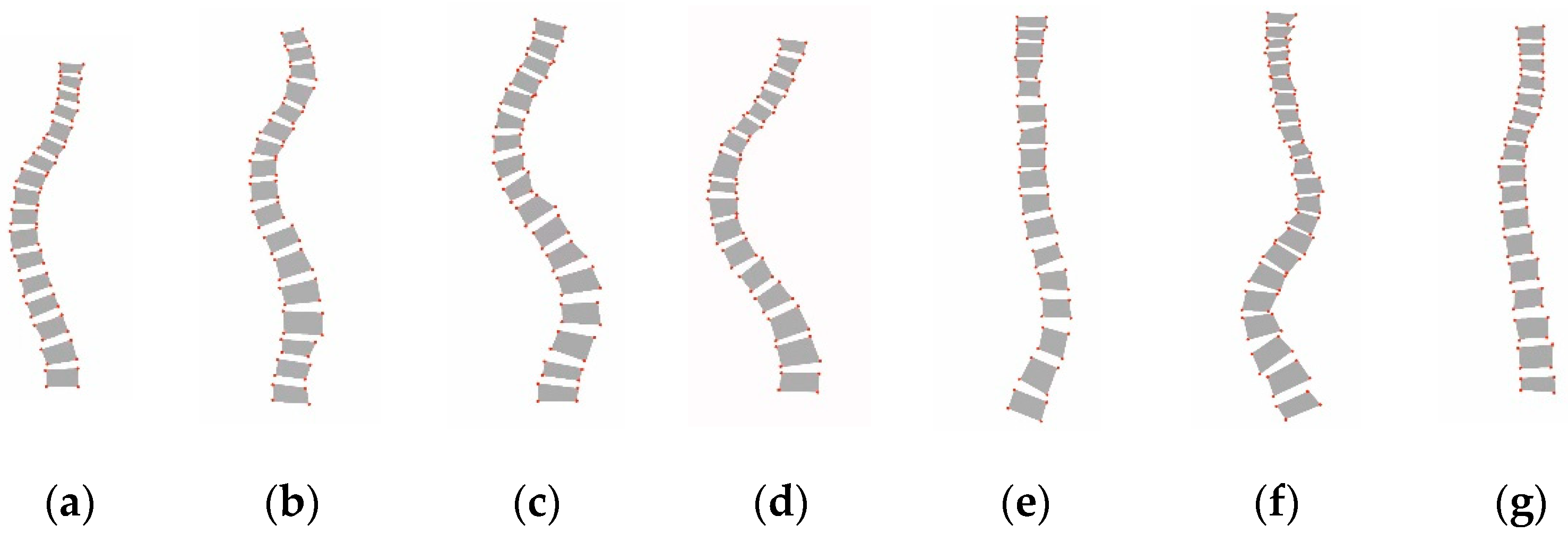
To further provide a visual comparison of the shape representation, we also conducted a content-based image retrieval experiment for the five compared shape descriptors. We input an original spine X-ray image as the query and retrieved the seven most similar results in the dataset using the proposed shape matching framework based segmentation network. The two groups of retrieval results are presented in Figure 16 and Figure 17, respectively.

From the above result, we can draw the following conclusions.

First, the proposed Lenke classification framework embedded with our adaptive shape descriptor achieves best results in all the evaluation indicators, which shows its outstanding performance compared with the other representative and latest methods. Specifically, compared with the shape context descriptor, we achieved an improvement of 35.8% in accuracy, 48.4% in precision, 37.5% in recall, and 43.1% in F1-score; compared with the Fourier descriptor, we achieved an improvement of 21.5% in accuracy, 20.9% in precision, 20.8% in recall, and 22.3% in F1-score. We also surpassed the other shape descriptors including CBoW and TAR for all metrics, and the improvement was markedly significant. This is mainly because our shape descriptor is especially designed for describing the microscopic shape distribution of the vertebrae, while the existing shape descriptors were mainly developed for objects with larger shape changes.

Second, we achieved superior results compared with deep learning classification methods. Specifically, compared with Resnet101, we achieved an improvement of 5.3% in accuracy, 20.8% in precision, 17.1% in recall, and 19.1% in F1-score. Compared to the recent transformer methods that demonstrated conspicuous performance in image classification, such as Swin transformer and vision transformer, we achieved more significant performance improvements. This demonstrates that the Lenke classification of scoliosis in X-rays is indeed challenging. It may be difficult to directly use an end-to-end deep learning method to the learn the small shape changes between different Lenke types, and our hand-designed method can better describe such shape differences. In addition, the small number of data samples affects the performance of transformers and other deep learning methods. We used deep leaning to segment and manually design the shape description and matching method to achieve a more efficient scoliosis classification.

Finally, by observing the content-based image retrieval results in Figure 16 and Figure 17, we found the proposed shape descriptor achieved the best results. Specifically, our method yielded the results that had the most Lenke types in common with the query. Using the query marked Lenke 4 in Figure 16 as an example, five of the seven most similar results by our method were Lenke 4, while, for the shape context, CBoW, TAR, and Fourier descriptor, there are four, four, three and two samples marked Lenke 4 were retrieved, respectively. For the results in Figure 17, our method also retrieved the most images, consistent with the Lenke type of the query. In addition, from the perspective of subjective observation, the results obtained using our method are more visually similar to the query, i.e., the shape of the spine obtained by our method is similar to that of the query. Even those results with different Lenke types from the query still have a certain similarity in the general outline shape. This implies that the proposed shape descriptor can describe the spine’s overall shape and local details well.

In summary, the proposed method achieved competitive performance in the Lenke classification of scoliosis.

3.6. Comparison of the Classification Framework Based on Cobb Angle Measurement and Shape Description

As shown in Figure 2, we present two alternative schemes for the Lenke classification of scoliosis. The first was to use Cobb angle measurement and classifying criteria (denoted as Cobb angle + criteria for short) based on the segmentation results, and the second was to use the shape description and KNN classifier (denoted as Shape + KNN for short) for the segmentation results. In this section, we conducted an experiment to compare the two schemes; the results are listed in

Table 7. Results of the classification framework based on Cobb angle measurement and shape description.

Compared Method	Segmentation Networks	Accuracy	Precision	Recall	F1-Score
Cobb angle + criteria	FPN	0.484	0.398	0.531	0.455
	PSPNet	0.428	0.376	0.691	0.487
	MANet	0.475	0.327	0.654	0.436
	Unet	0.486	0.388	0.559	0.458
	Segmenter	0.373	0.304	0.469	0.369
	Unet++	0.489	0.352	0.685	0.465
Shape descriptor + KNN	FPN	0.712	0.742	0.616	0.673
	PSPNet	0.675	0.758	0.517	0.615
	MANet	0.682	0.706	0.534	0.608
	Unet	0.697	0.715	0.616	0.662
	Segmebter	0.731	0.731	0.630	0.677
	Unet++	0.786	0.804	0.756	0.779

.

From Table 7, we note that the scheme using the shape description and KNN classifier achieved better experimental results than that using the Cobb angle and classifying criteria, where most of the indicators are significant. This is because the Lenke classification criteria built on the Cobb angle is very strict and is extremely dependent on the accuracy of the segmentation. However, the proposed automatic Lenke classification method based on the shape descriptor and KNN classifier achieved a considerable improvement and overcame the influence of the segmentation error caused by deep learning to a great extent.

3.7. Computational Complexity Analysis

In this section, we focus on computational complexity analysis for the proposed Lenke classification framework of scoliosis, which consists of two parts: segmentation using deep learning and classification using the shape descriptor and classifier.

First, we report the parameter memory as the evaluation indicator for the segmentation networks in

Table 8. Computational complexities of segmentation networks.

Networks	FPN	PSPNet	MANet	Unet	Segmenter	Unet++
Params	28.51 M	49.01 M	19.42 M	29.05 M	25.74 M	34.96 M

, in which the input and output image are resized to 256 * 256. To provide a more intuitive and comprehensive comparison, a schematic diagram of the computational complexity requirements vs. the classification performance is presented in Figure 18. From the above results, the MANet evidently has the smallest params. However, if we regard the classification performance as a comprehensive consideration, the Unet++ has a moderate param size and operation count. Therefore, based on a balance of the classification and time complexity, we recommend Unet++ as the preferred segmentation network.

Next, we performed computational complexity analysis for different classification methods, which mainly included feature extraction, training, and testing. From the results shown in

Table 9. Time consumption with different classification methods.

Methods	Feature Extraction	Training	Testing
Shape context	882.226 s	/	6.623 s
CBoW	12.021 s	98.53 s	2.157 s
TAR	52.175 s	/	6.248 s
Fourier descriptor	5.136 s	/	4.278 s
Swin transformer	/	447.10 s	0.137 s
Vision transformer	/	4979.01 s	0.132 s
Resnet101	/	933.02 s	0.130 s
OURS	0.983 s	/	0.889 s

, the proposed adaptive shape descriptor had minimum time consumption in the feature extraction among all shape descriptors and a moderate testing time. It is worth noting that shape context, TAR, and our method directly extracted features from a single image. Thus, there is no training process. For CBoW, the visual dictionary needs to be trained from the dataset, and the training time is relatively long. For deep learning methods, the feature extraction is included in the training time. Considering the actual performance and time complexity, we concluded that the proposed method is the best choice in the Lenke classification of scoliosis.

4. Conclusions and Future Perspectives

In this study, we mainly investigated the Lenke classification problem for scoliosis and proposed a novel automatic Lenke classification framework. First, we used deep networks such as Unet++ to segment the vertebrae in the spine X-ray images and employed an effective post-processing strategy to overcome the spots and adhesions caused by the segmentation errors. We then focused on the shape representation of the segmented spine, and a new shape descriptor was designed to describe the details of the spinal curvature. With shape feature extraction and matching, a new Lenke classification algorithm for scoliosis was constructed with a classifier. For comparison and application, we also built another alternative Lenke classification option based on the automatic measurement of the Cobb angle. Finally, multiple experiments were conducted on a public dataset, including evaluating the segmentation networks, evaluating the shape descriptors, evaluating the classification strategies, and performing ablation experiments. The experimental results indicated that the proposed method achieved the best Lenke classification performance for scoliosis among the compared methods. The ablation experiments demonstrated that the modules in our shape descriptor were organically connected and supported by each other.

To further highlight the technical improvements and contribution compared with the state-of-the-art methods, three aspects should be noted. First, we improved the overall framework and viewed the Lenke classification of scoliosis from the perspective of its microscopic shape on the basis of segmentation network. Second, we improved the shape representation through three novel strategies: the adaptive similarity matching based on key segment calculation, the tilt angle description, and the symmetric matching. These strategies are carefully designed for the needs of the Lenke classification of scoliosis, which can be used to obtain more shape details. Finally, a general post-processing method for vertebrae segmentation is proposed, which improved the segmentation results for all compared deep networks.

Although the proposed method achieved superior results in the Lenke classification of scoliosis, there is still much room for improvement in terms of the objective evaluation indicators. This is attributed to two reasons. First, different Lenke types have very similar shapes, which is very hard to distinguish with human judgment. The rules of the Lenke classification dictate that it requires a very high level of segmentation and fine-grained shape representation, which is a great challenge. In addition, for fairness of the comparison and reproducibility of the results, we evaluated our method on a publicly available dataset that only included coronal plane X-rays of scoliosis. In fact, sagittal plane X-rays are an important supplement for diagnosing of scoliosis. However, under the present case, our method still significantly improved the existing methods and yielded satisfactory results with smaller data requirements, faster computation, and full automation. Moreover, the proposed Lenke classification framework and adaptive shape descriptor are also applicable to evaluating the spinal curvature of the sagittal plane X-rays. Combining the coronal plane and sagittal plane X-rays can further improve the proposed method’s performance. One alternative solution is to assign the weights to the coronal and sagittal plane X-rays in the similarity matching of the two scoliosis cases. In future work, we will construct a clinical scoliosis dataset with both sagittal and coronal plane X-rays and fully utilize two kinds of plane information to further improve the Lenke classification of scoliosis.

References

1. Cheng, J.C.; Castelein, R.M.; Chu, W.C.; Danielsson, A.J.; Dobbs, M.B.; Grivas, T.B.; Gurnett, C.A.; Luk, K.D.; Moreau, A.; Newton, P.O.; et al. Adolescent idiopathic scoliosis. Nat. Rev. Dis. Prim. 2015, 1, 15030. [Google Scholar] [CrossRef] [Green Version]
2. Konieczny, M.R.; Senyurt, H.; Krauspe, R. Epidemiology of adolescent idiopathic scoliosis. J. Child. Orthop. 2013, 7, 3–9. [Google Scholar] [CrossRef] [PubMed] [Green Version]
3. Hresko, M.T. Idiopathic Scoliosis in Adolescents. N. Engl. J. Med. 2013, 368, 834–841. [Google Scholar] [CrossRef] [PubMed]
4. Lenke, L.G.; Betz, R.R.; Harms, J.; Bridwell, K.H.; Clements, D.H.; Lowe, T.G.; Blanke, K. Adolescent idiopathic scoliosis: A new classification to determine extent of spinal arthrodesis. J. Bone Jt. Surg. 2001, 83, 1169–1181. [Google Scholar] [CrossRef]
5. Ronneberger, O.; Fischer, P.; Brox, T. U-Net: Convolutional Networks for Biomedical Image Segmentation. In Proceedings of the International Conference on Medical Image Computing and Computer-Assisted Intervention, Munich, Germany, 5–9 October 2015; Springer: Cham, Switzerland, 2015; pp. 234–241. [Google Scholar]
6. Long, J.; Shelhamer, E.; Darrell, T. Fully Convolutional Networks for Semantic Segmentation. In Proceedings of the IEEE Conference on Computer Vision and Pattern Recognition, Boston, MA, USA, 7–12 June 2015; pp. 3431–3440. [Google Scholar]
7. Zhou, Z.; Siddiquee, M.M.R.; Tajbakhsh, N.; Liang, J. Unet++: Redesigning Skip Connections to Exploit Multiscale Features in Image Segmentation. IEEE Trans. Med. Imaging 2019, 39, 1856–1867. [Google Scholar] [CrossRef] [PubMed] [Green Version]
8. Fan, T.; Wang, G.; Li, Y.; Wang, H. MA-Net: A Multi-Scale Attention Network for Liver and Tumor Segmentation. IEEE Access 2020, 8, 179656–179665. [Google Scholar] [CrossRef]
9. Khan, R.A.; Luo, Y.; Wu, F.X. RMS-UNet: Residual multi-scale UNet for liver and lesion segmentation. Artif. Intell. Med. 2022, 124, 102231. [Google Scholar] [CrossRef]
10. Chi, J.; Han, X.; Wu, C.; Wang, H.; Ji, P. X-Net: Multi-branch UNet-like network for liver and tumor segmentation from 3D abdominal CT scans. Neurocomputing 2021, 459, 81–96. [Google Scholar] [CrossRef]
11. Li, Y.; Si, Y.; Tong, Z.; He, L.; Zhang, J.; Luo, S.; Gong, Y. MQANet: Multi-Task Quadruple Attention Network of Multi-Object Semantic Segmentation from Remote Sensing Images. Remote Sens. 2022, 14, 6256. [Google Scholar] [CrossRef]
12. Al Arif, S.M.M.R.; Knapp, K.; Slabaugh, G. Fully automatic cervical vertebrae segmentation framework for X-ray images. Comput. Methods Programs Biomed. 2018, 157, 95–111. [Google Scholar] [CrossRef] [Green Version]
13. Banerjee, S.; Lyu, J.; Huang, Z.; Leung, F.H.; Lee, T.; Yang, D.; Su, S.; Zheng, Y.; Ling, S.H. Ultrasound spine image segmentation using multi-scale feature fusion Skip-Inception U-Net (SIU-Net). Biocybern. Biomed. Eng. 2022, 42, 341–361. [Google Scholar] [CrossRef]
14. Payer, C.; Tern, D.; Bischof, H.; Urschler, M. Coarse to Fine Vertebrae Localization and Segmentation with Spatial Configuration-Net and U-Net. In Proceedings of the 15th International Joint Conference on Computer Vision, Imaging and Computer Graphics Theory and Applications, Valletta, Malta, 27–29 February 2020; Volume 100, pp. 124–133. [Google Scholar]
15. Sekuboyina, A.; Husseini, M.E.; Bayat, A.; Löffler, M.; Liebl, H.; Li, H.; Tetteh, G.; Kukačka, J.; Payer, C.; Štern, D.; et al. VerSe: A Vertebrae Labelling and Segmentation Benchmark for Multi-detector CT Images. Med. Image Anal. 2021, 73, 102166. [Google Scholar] [CrossRef]
16. Ranftl, R.; Bochkovskiy, A.; Koltun, V. Vision Transformers for Dense Prediction. In Proceedings of the IEEE/CVF International Conference on Computer Vision, Online, 11–17 October 2021; pp. 12179–12188. [Google Scholar]
17. Strudel, R.; Garcia, R.; Laptev, I.; Schmid, C. Segmenter: Transformer for Semantic Segmentation. In Proceedings of the IEEE/CVF International Conference on Computer Vision, Online, 11–17 October 2021; pp. 7262–7272. [Google Scholar]
18. Dosovitskiy, A.; Beyer, L.; Kolesnikov, A.; Weissenborn, D.; Zhai, X.; Unterthiner, T.; Dehghani, M.; Minderer, M.; Heigold, G.; Gelly, S.; et al. An Image is Worth 16 × 16 Words: Transformers for Image Recognition at Scale. In Proceedings of the International Conference on Learning Representations, Online, 3–7 May 2021. [Google Scholar]
19. Tao, R.; Liu, W.; Zheng, G. Spine-transformers: Vertebra labeling and segmentation in arbitrary field-of-view spine CTs via 3D transformers. Med. Image Anal. 2022, 75, 102258. [Google Scholar] [CrossRef]
20. Wang, L.; Xie, C.; Lin, Y.; Zhou, H.Y.; Chen, K.; Cheng, D.; Dubost, F.; Collery, B.; Khanal, B.; Khanal, B.; et al. Evaluation and Comparison of Accurate Automated Spinal Curvature Estimation Algorithms with Spinal Anterior-posterior X-ray Images: The AASCE2019 Challenge. Med. Image Anal. 2021, 72, 102115. [Google Scholar] [CrossRef]
21. Zhang, C.; Wang, J.; He, J.; Gao, P.; Xie, G. Automated vertebral landmarks and spinal curvature estimation using non-directional part affinity fields. Neurocomputing 2021, 438, 280–289. [Google Scholar] [CrossRef]
22. Lin, Y.; Zhou, H.Y.; Ma, K.; Yang, X.; Zheng, Y. Seg4Reg Networks for Automated Spinal Curvature Estimation. In Proceedings of the International Workshop and Challenge on Computational Methods and Clinical Applications for Spine Imaging, Shenzhen, China, 17 October 2019; pp. 69–74. [Google Scholar]
23. Kim, K.C.; Yun, H.S.; Kim, S.; Seo, J.K. Automation of spine curve assessment in frontal radiographs using deep learning of vertebral-tilt vector. IEEE Access 2020, 8, 84618–84630. [Google Scholar] [CrossRef]
24. Bayat, A.; Sekuboyina, A.; Hofmann, F.; Husseini, M.E.; Kirschke, J.S.; Menze, B.H. Vertebral labelling in radiographs: Learning a coordinate corrector to enforce spinal shape. In Proceedings of the International Workshop and Challenge on Computational Methods and Clinical Applications for Spine Imaging, Shenzhen, China, 17 October 2019; Springer: Cham, Switzerland, 2020; pp. 39–46. [Google Scholar]
25. Tan, Z.; Yang, K.; Sun, Y.; Wu, B.; Li, S.; Hu, Y.; Tao, H. An Automatic Classification Method for Adolescent Idiopathic Scoliosis Based on U-net and Support Vector Machine. J. Imaging Sci. Technol. 2019, 63, 60502. [Google Scholar] [CrossRef]
26. Yang, D.; Lee, T.; Lai, K.; Wong, Y.; Wong, L.; Yang, J.; Lam, T.; Castelein, R.; Cheng, J.; Zheng, Y. A novel classification method for mild adolescent idiopathic scoliosis using 3D ultrasound imaging. Med. Nov. Technol. Devices 2021, 11, 100075. [Google Scholar] [CrossRef]
27. Yang, D.; Lee, T.T.Y.; Lai, K.K.L.; Lam, T.P.; Castelein, R.M.; Cheng, J.C.Y.; Zheng, Y.P. Semi-automatic method for pre-surgery scoliosis classification on X-ray images using Bending Asymmetry Index. Int. J. Comput. Assist. Radiol. Surg. 2022, 17, 2239–2251. [Google Scholar] [CrossRef] [PubMed]
28. Gardner, A.; Berryman, F.; Pynsent, P. A cluster analysis describing spine and torso shape in Lenke type 1 adolescent idiopathic scoliosis. Eur. Spine J. 2021, 30, 620–627. [Google Scholar] [CrossRef] [PubMed]
29. Rothstock, S.; Weiss, H.R.; Krueger, D.; Paul, L. Clinical classification of scoliosis patients using machine learning and markerless 3D surface trunk data. Med. Biol. Eng. Comput. 2020, 58, 2953–2962. [Google Scholar] [CrossRef] [PubMed]
30. Zhang, J.; Shi, X.; Lv, L.; Wang, X.; Zhang, Y.; Guo, F. Computerized Lenke classification of scoliotic spine. In Proceedings of the 2013 35th Annual International Conference of the IEEE Engineering in Medicine and Biology Society (EMBC), Osaka, Japan, 3–7 July 2013; pp. 945–948. [Google Scholar]
31. Jin, C.; Wang, S.; Yang, G.; Li, E.; Liang, Z. A Review of the Methods on Cobb Angle Measurements for Spinal Curvature. Sensors 2022, 22, 3258. [Google Scholar] [CrossRef]
32. Logithasan, V.; Wong, J.; Reformat, M.; Lou, E. Using machine learning to automatically measure axial vertebral rotation on radiographs in adolescents with idiopathic scoliosis. Med. Eng. Phys. 2022, 107, 103848. [Google Scholar] [CrossRef] [PubMed]
33. Goldstein, M. k_n-nearest neighbor classification. IEEE Trans. Inf. Theory 1972, 18, 627–630. [Google Scholar] [CrossRef]
34. Canny, J. A Computational Approach to Edge Detection. IEEE Trans. Pattern Anal. Mach. Intell. 1986, 8, 679–698. [Google Scholar] [CrossRef] [PubMed]
35. Wu, H.; Bailey, C.; Rasoulinejad, P.; Li, S. Automatic landmark estimation for adolescent idiopathic scoliosis assessment using boostnet. In Proceedings of the Medical Image Computing and Computer Assisted Intervention, Quebec City, QC, Canada, 11–13 September 2017; pp. 127–135. [Google Scholar]
36. MMSegmentation: OpenMMLab Semantic Segmentation Toolbox and Benchmark. GitHub Repository. 2020. Available online: https://github.com/open-mmlab/mmsegmentation (accessed on 11 February 2023).
37. Iakubovskii, P. Segmentation Models Pytorch. GitHub Repository. 2019. Available online: https://github.com/qubvel/segmentation_models.pytorch (accessed on 11 February 2023).
38. Wang, Z.B.; Wang, E.; Zhu, Y. Image segmentation evaluation: A survey of methods. Artif. Intell. Rev. 2020, 53, 5637–5674. [Google Scholar] [CrossRef]
39. Kirillov, A.; Girshick, R.; He, K.; Dollár, P. Panoptic Feature Pyramid Networks. In Proceedings of the IEEE Conference on Computer Vision and Pattern Recognition (CVPR), Long Beach, CA, USA, 16–20 June 2019. [Google Scholar]
40. Zhao, H.; Shi, J.; Qi, X.; Wang, X.; Jia, J. Pyramid Scene Parsing Network. In Proceedings of the IEEE Conference on Computer Vision and Pattern Recognition (CVPR), Honolulu, HI, USA, 21–26 July 2017. [Google Scholar]
41. Belongie, S.J.; Malik, J.M.; Puzicha, J. Shape Matching and Object Recognition Using Shape Contexts. IEEE Trans. Pattern Anal. Mach. Intell. 2002, 24, 509–522. [Google Scholar] [CrossRef] [Green Version]
42. Ling, H.; Jacobs, D.W. Using the Inner-Distance for Classification of Articulated Shapes. In Proceedings of the IEEE Computer Society Conference on Computer Vision and Pattern Recognition, San Diego, CA, USA, 20–25 June 2005. [Google Scholar]
43. Alajlan, N.; Kamel, M.S.; Freeman, G.H. Geometry-Based Image Retrieval in Binary Image Databases. IEEE Trans. Pattern Anal. Mach. Intell. 2008, 30, 1003. [Google Scholar] [CrossRef]
44. Zeng, J.; Liu, M.; Fu, X.; Gu, R.; Leng, L. Curvature Bag of Words Model for Shape Recognition. IEEE Access 2019, 7, 57163–57171. [Google Scholar] [CrossRef]
45. Liu, H.; Rashid, T.; Habes, M. Cerebral Microbleed Detection Via Fourier Descriptor with Dual Domain Distribution Modeling. In Proceedings of the IEEE 17th International Symposium on Biomedical Imaging Workshops, Iowa City, IA, USA, 4 April 2020. [Google Scholar]
46. He, K.; Zhang, X.; Ren, S.; Sun, J. Deep residual learning for image recognition. In Proceedings of the IEEE Conference on Computer Vision and Pattern Recognition (CVPR), Las Vegas, NV, USA, 26 June–1 July 2016; pp. 770–778. [Google Scholar]
47. Liu, Z.; Lin, Y.; Cao, Y.; Hu, H.; Wei, Y.; Zhang, Z.; Lin, S.; Guo, B. Swin Transformer: Hierarchical Vision Transformer using Shifted Windows. In Proceedings of the IEEE/CVF International Conference on Computer Vision (ICCV), Online, 11–17 October 2021. [Google Scholar]
Figure 1. The normal spine and six Lenke types of scoliosis: (a) Lenke 1; (b) Lenke 2; (c) Lenke 3; (d) Lenke 4; (e) Lenke 5; (f) Lenke 6; and (g) normal.
Applsci 13 03905 g001
Figure 2. An overview of the proposed method.
Applsci 13 03905 g002
Figure 3. The deep network models for segmentation: (a) Unet architecture; (b) Unet++ architecture.
Applsci 13 03905 g003
Figure 4. The post-processing for segmentation result.
Applsci 13 03905 g004
Figure 5. An example for calculating average fluctuation angle of sampling points of the segmented vertebra. (a0, a1, …, a9) are sampled points; θ i j denotes the angle between ai and its j-th neighbor on the left and right; θ ¯ i denotes the average fluctuation angle of ai.
Applsci 13 03905 g005
Figure 6. Automatic measurement of Cobb angle. L1[i] denotes the slope of the straight line representing the superior endplate of the i-th vertebra; L2[i] denotes the slope of the straight line representing the inferior endplate of the i-th vertebra; H(i,j) denotes the angle between the superior endplate of the i-th vertebra and the the inferior endplate of the j-th vertebra.
Applsci 13 03905 g006
Figure 7. Outline representation using shape encoding. (a) Circular direction template; (b) outline representation of vertebrae.
Applsci 13 03905 g007
Figure 8. Examples for key segments in the segmented spinal image.
Applsci 13 03905 g008
Figure 9. Examples of vertebrae with different tilt angles.
Applsci 13 03905 g009
Figure 10. Example of symmetric matching.
Applsci 13 03905 g010
Figure 11. The automatic scoliosis Lenke classification algorithm based on Cobb angle measurement. PT c denotes the Cobb angle of proximal thoracic in the coronal plane; PT s denotes the Cobb angle of proximal thoracic in the sagittal plane; MT c denotes the Cobb angle of main thoracic in the coronal plane; MT s denotes the Cobb angle of main thoracic in the sagittal plane; TL c denotes the Cobb angle of thoracolumbar/lumbar in the coronal plane; TL s denotes the Cobb angle of thoracolumbar/lumbar in the sagittal plane.
Applsci 13 03905 g011
Figure 12. A block diagram of the calculation process of Lenke classification based on shape descriptor.
Applsci 13 03905 g012
Figure 13. The examples of original image samples.
Applsci 13 03905 g013
Figure 14. The visual comparison of different segmentation networks. GT: ground truth.
Applsci 13 03905 g014
Figure 15. The visual comparison of some examples to illustrate the effects of post-processing. GT: ground truth; Predict: without post-processing; OURS: the post-processing was used.
Applsci 13 03905 g015
Figure 16. Image retrieval example for different shape descriptors with the query of Lenke 4.
Applsci 13 03905 g016aApplsci 13 03905 g016b
Figure 17. Image retrieval example for different shape descriptors with the query of Lenke 0.
Applsci 13 03905 g017aApplsci 13 03905 g017b
Figure 18. Computational complexity requirements vs. classification performance. (a) Accuracy versus param size; (b) precision versus param size; (c) recall versus param size; and (d) F1-score versus param size.
Applsci 13 03905 g018