Formation of a Lightweight, Deep Learning-Based Weed Detection System for a Commercial Autonomous Laser Weeding Robot

Abstract

Weed management is becoming increasingly important for sustainable crop production. Weeds cause an average yield loss of 11.5% billion in Pakistan, which is more than PKR 65 billion per year. A real-time laser weeding robot can increase the crop’s yield by efficiently removing weeds. Therefore, it helps decrease the environmental risks associated with traditional weed management approaches. However, to work efficiently and accurately, the weeding robot must have a robust weed detection mechanism to avoid physical damage to the targeted crops. This work focuses on developing a lightweight weed detection mechanism to assist laser weeding robots. The weed images were collected from six different agriculture farms in Pakistan. The dataset consisted of 9000 images of three crops: okra, bitter gourd, sponge gourd, and four weed species (horseweed, herb paris, grasses, and small weeds). We chose a single-shot object detection model, YOLO5. The selected model achieved a mAP of 0.88@IOU 0.5, indicating that the model predicted a large number of true positive (TP) with much less prediction of false positive (FP) and false negative (FN). While SSD-ResNet50 achieved a mAP of 0.53@IOU 0.5, the model predicted fewer TP with significant outcomes as FP or FN. The superior performance of the YOLOv5 model made it suitable for detecting and classifying weeds and crops within fields. Furthermore, the model was ported to an Nvidia Xavier AGX standalone device to make it a high-performance and low-power computation detection system. The model achieved an FPS rate of 27. Therefore, it is highly compatible with the laser weeding robot, which takes approximately 22.04 h at a velocity of 0.25 feet per second to remove weeds from a one-acre plot.

1. Introduction

Agriculture plays a vital role in the economy of Pakistan, contributing to around 23.13% of the GDP [1]. It employs 43.5% of the workforce and contributes significantly to the country’s socioeconomic development [2]. A variety of biotic and abiotic factors limit crop yields around the world [3]. The most damaging biotic constraints to agricultural production are weeds. It competes with crops for moisture, nutrients, and sunlight, which ultimately reduces crop yield [3]. Global grain production is currently 2.1 billion tons. Weeds cause a 10% decrease in overall yield each year [4]. Depending on their species and densities, weeds cause an average yield loss of 11.5% in Pakistan, which is over PKR 65 billion annually [5].

Although traditional weed removal technology is playing its role in the control of weeds in agricultural fields [6]. Weeds can reduce production by more than 90% if they are not controlled. When traditional weed removal technology is used, grain production losses average 10–15% [7]. However, they have raised significant concerns because of their impact on the environment and their labor-intensive nature [8]. In chemical-based weed control, a single pesticide dose is sprayed over the entire field, uniformly covering the soil, crops, and weeds [9]. This widespread and uniform application of herbicides not only causes air pollution but also enters human and animal bodies through the food chain [10], therefore causing significant ecological and health damage. Glyphosate, a widely used herbicide, has been classified as carcinogenic for humans by the World Health Organization (WHO) in 2015 [6]. Assessing the damage caused by chemical weeding technology, there is a pressing need to create a robust weed management system that is efficient, cost-effective, and environmentally friendly [11].

Artificial intelligence has revolutionized several industries, including agriculture, since the start of the Fourth Industrial Revolution [12]. Many advanced, nondestructive techniques for agricultural field management have been developed [13]. Presently, computer vision and global positioning system (GPS) technology are used to perform many agriculture tasks smartly [14]. Some of these are crop yield prediction, plant disease detection, species identification, water, and soil conservation. As a result, variable rate input applications and precise and timely field action are now possible [15]. Recently, deep learning (DL) techniques have been used to detect weeds within and between crop rows. Weed detection and classification are complicated by the fact that in their early stages, weeds and crops have extremely similar colors and textures [16]. ML-based systems are being proposed to distinguish crops from weeds in real time. These systems help to control weeds effectively, but they cannot be fully adopted by a grass-roots farmer until low-cost, precise weed-detection systems are developed [17]. Crop damage can result from poor precision [18].

Machine learning algorithms extract features from input data, such as shape, texture, and color [19]. Conventional ML techniques need substantial domain knowledge to construct a feature extractor based on the shape and texture associated with each type of weed [20]. The deep learning approach on the other hand, employs a representational learning method [21]. In DL, a machine recognizes discriminative features from input data and extracts the features that are best for automatic classification and object detection tasks [22]. Due to their strong feature learning abilities, DL algorithms have a number of advantages over typical machine learning methods. Convolutional neural networks (CNNs) and recurrent neural networks (RNNs) are two commonly used and high-performing network architectures available in DL [22]. CNN is built on a stack of convolutional layers. Each layer takes in the incoming data, transforms or convolves it, and then sends it to the next layer [23]. To date, approaches based on CNNs, such as object detection models, are the most efficient models for weed detection [24]. The most advanced CNN-based object detection models can be divided into two categories: (a) a two-stage approach; and (b) a one-stage approach [24]. A one-stage approach, as compared to a two-stage approach, only needs one pass through the neural network to predict all the bounding boxes [25]. This is much faster and more suitable for real-time applications [25]. You only look once (YOLO) is a one-stage object detection system that generates bounding boxes and class predictions after only one image evaluation [26]. Another one-stage objection detection model that has been used in the literature is the single-shot multibox detector residual network (SSD-Resnet) [27].

A DL-based lightweight weed detection system is presented to address the practical challenges of detecting weeds in real-time within crops.The system will detect and classify weeds in fields to assist an autonomous laser-based weed-killing vehicle. The main contributions of the work are as follows:

• A lightweight deep learning model is developed for a commercial autonomous laser weeding robot to kill weeds in real time.
• A large dataset was created by visiting several local farming fields in the area of Gadap town in Karachi, with the goal of collecting data of the most common weeds and the crops of Gadap town. As a result, a model trained on this data is more robust for this selected field.
• Single-shot object detection models, YOLOv5 and SSD-RestNet, are used to detect and classify crops and weeds. The YOLO model’s high performance in terms of its inference time in frame extraction and detection makes it an ideal model for weed detection systems.
• The model is implemented on a Nvidia Xavier AGX embedded device [28] to make it a high-performance and low-power standalone detection system.

2. Literature Review

This section provides an extensive review of machine learning techniques used for the development of weed detection and classification systems.

Many cutting-edge deep learning models for weed classification, such as VGG-16, CNN, NN, and random forest regression, have been proposed [29,30,31,32]. Sethia et al. proposed a system for weed detection and image processing. The convolutional neural network (VGG16) was used, which shows 99.5% precision while classifying leaf species. The system generated good results, but there is room for development. Plant identification can be improved with a more robust algorithm that can distinguish more species of leaves regardless of color or form [29]. To identify weed locations in the field for precise killing without damaging the crops, a faster RCNN network, an object detection model, was applied by Longzhe et al. for distinguishing weed and maize seedlings. The model detected weeds with 97.71% precision under three conditions: full-cycle, multi-weather and multi-angle. The model can only be used on maize farms, which limits its application. Furthermore, the detection speed of Faster RCNN was 7 frames per second, which is low for real-time weed detection [33].

YOLO is a one-stage approach for detecting objects. It improves object detection speed by performing a CNN architecture on the image to determine the position and type of the objects in the image. The first YOLO version was introduced by Wang et al. in 2015 [34]. Many improved versions of YOLO, such as YOLOv1, YOLOv2, YOLOv3, YOLOv4, and YOLOv5, have been developed in recent years [35]. There are various improvements in architecture from YOLOv1 to YOLOv5. The first version of YOLO was detected through grid division but had low confidence. YOLO2 works with k-means anchor boxes. Whereas YOLO3 uses the feature pyramid network (FPN), YOLO4 is added with the generalized intersection over union (GIOU) loss function, the MISH activation function, and data enhancement through the mosaic mixup method [35]. YOLO5 is distinct from all previous releases. The most significant enhancements are mosaic data augmentation and auto-learning bounding box anchors [34].

Previous versions of YOLO have been extensively studied for application in weed detection. Mahmoud et al. implemented a deep weed detector/classifier for precision agriculture using the YOLOv2 fused with the ResNet-50 object detection model. Except for the sedge weed, their model achieved precision and recall of over 94% for each weed class. As they used an older version of YOLO2, it lacks an auto-learning bounding box anchor [36]. Sanchez et al. compared three one-staged object detection models: YOLO-V4, YOLO5, and SSD MobileNet V2. The dataset consisted of 153 RGB images of onion plants. According to the study, YOLO5 performed significantly well. It consumed significantly fewer resources, making it suitable for real-time weed detection. At 0.195 mAP, it showed less mean inference time of 7.72 milliseconds as compared to the other two models. This study demonstrated that up-sizing the data through sample augmentation will produce better results [37].

In 2022, Xiojun Jin et al. evaluated three cutting-edge CNN-based architectures, You Only Look Once-v3 (YOLO3), CenterNet, and Faster R-CNN, for bok choy, also known as Chinese white cabbage, detection. The most accurate model for vegetable recognition was YOLO3, which had the highest F1 score of 0.971 as well as high precision and recall values of 0.971 and 0.970, respectively. YOLO3 had a similar inference time to CenterNet, but was substantially faster than Faster R-CNN. Overall, YOLO3 had the best accuracy and computational efficiency of the deep-learning architectures studied [38].

Scott et al. compared the performance of the SSD model with the faster RCNN in 2020. The dataset contained UAV images of weeds collected from mid to late-season soybean fields. The models were evaluated based on values of mean intersection over union (IoU) and inference speed. The study concluded that the SSD model had similar precision, recall, f1 score, IoU, and inference time values compared to the Faster RCNN. However, the optimal SSD confidence threshold was found to be 0.1, indicating that this model has less confidence when weed objects are detected. Moreover, the SSD model incorrectly identified a row of herbicide-damaged soybean fields as weeds. Additionally, SSD was unable to identify the weeds on the image’s left vertical edge. These failures identify the susceptibility of the SSD model in the border areas of the image [39].

Olaniyi et al. used a single-shot multi-box detector (SSD) for detecting weeds in the fields. The overall system accuracy was 86%. In addition, the algorithm had a 93% system sensitivity and an 84% precision value. However, the model struggled to detect very small weeds that appeared in the corners of the images [40].

YOLOv5 achieves real-time performance [41], which is selected in this study by comparing its performance with another object detection model, SSD-ResNet. The performance of YOLOv5 in detecting and classifying weeds and crops makes it a suitable model for the system.

3. Methodology

The mechanism of the weed detection system is discussed in this section.The steps followed in the development of the weed detection system are illustrated in Figure 1. Each head is described in detail in the subsequent sections of the paper.

3.1. Data Acquisition

To begin, field surveys were conducted in six agriculture fields across Pakistan, including Thatta, Mirpur Khas, Darsano Chano, Gaddap, Quetta, and Rahim Yar Khan. The goal was to connect with farmers, gain an understanding of the surrounding environment, and collect images of weeds in the fields.

Establishment of the Real-Time Experimental Setup for Data Acquisition

The primary data came from the Agro Living Lab (ALL), located in the Gadap region of Karachi. The purpose of establishing ALL was to allow researchers to collect authentic data without encountering obstacles. It can be difficult to obtain permission from farmers and landowners to photograph their fields. The Living Lab also facilitated quantifying and analyzing the types of weeds that are commonly found and the crops that are commonly cultivated in that particular land of Gadap town. Furthermore, the furrow irrigation system was designed to allow weeding robots to move freely without harming crops.

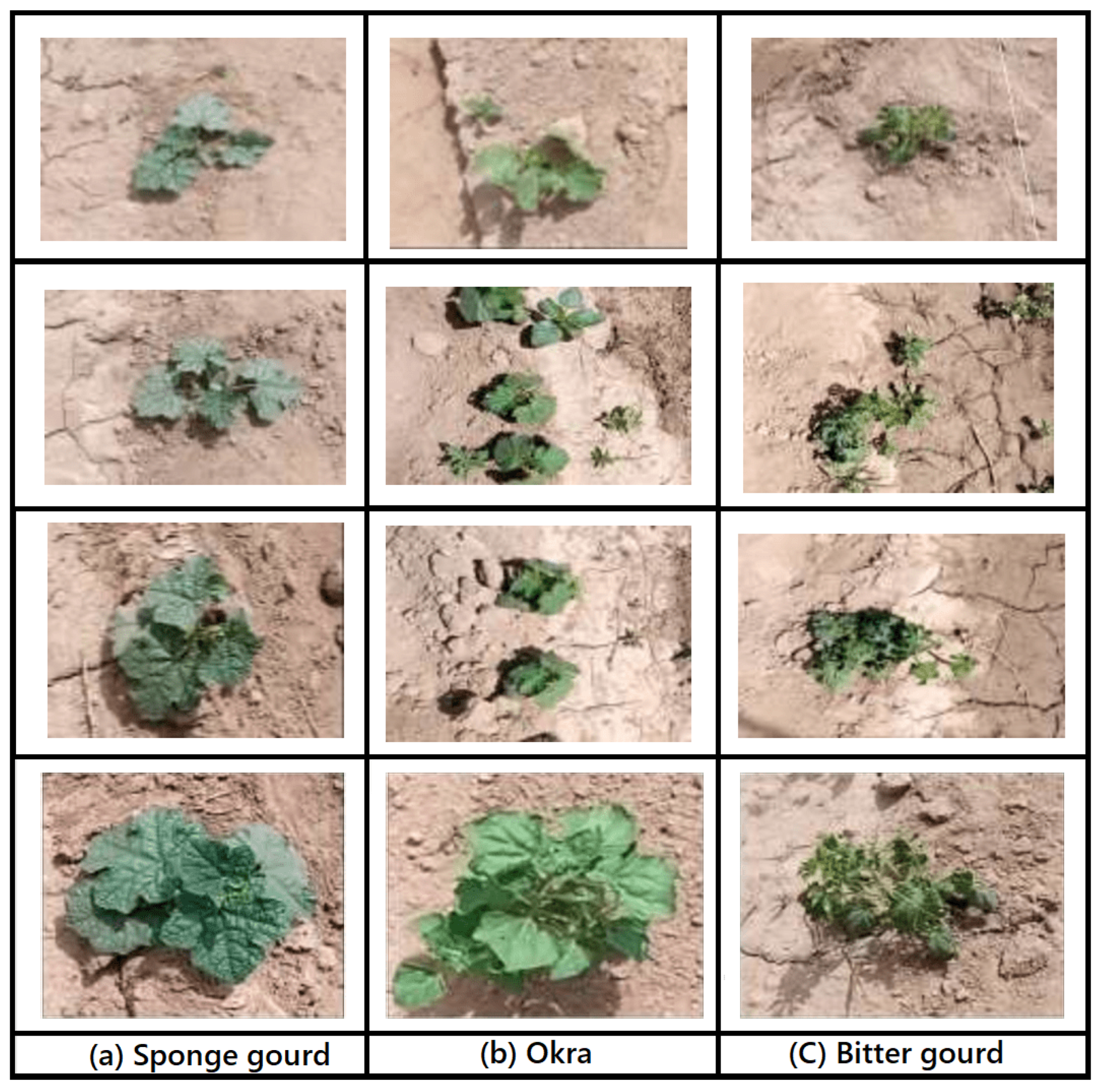
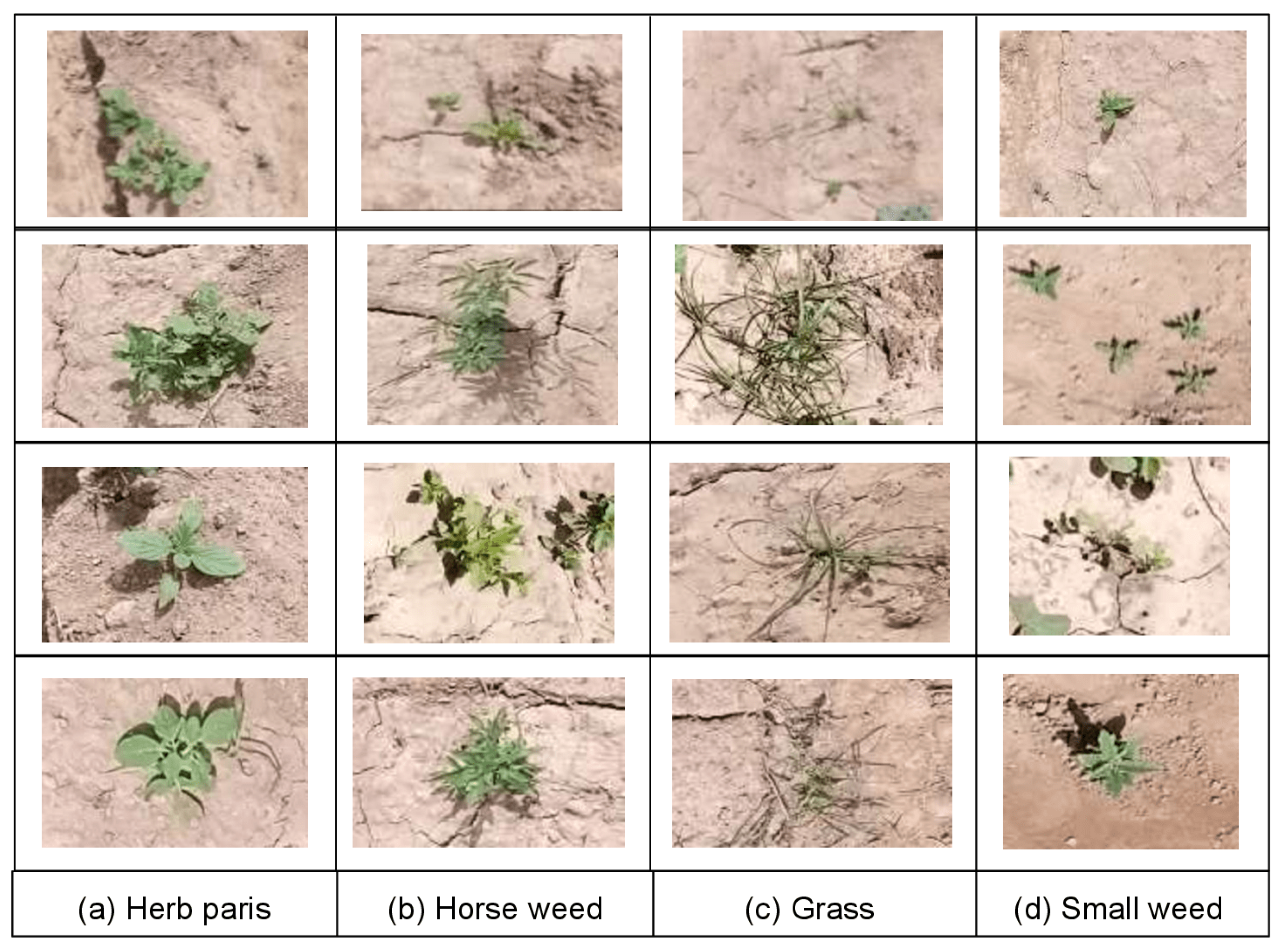
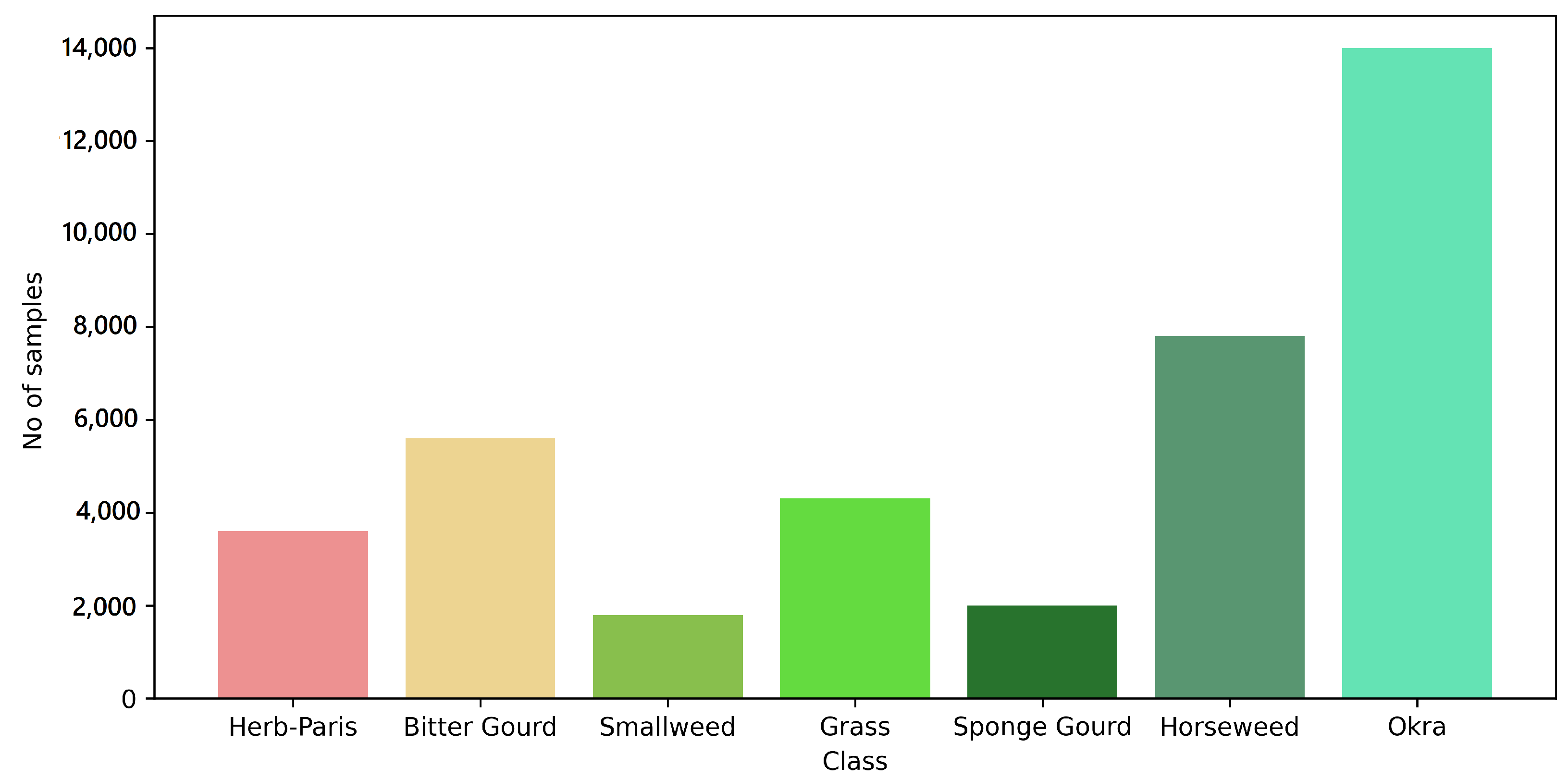
The dataset was collected in the form of videos, and 12,000 frames were extracted from the videos acquired through a 60 fps camera. The resolution of the camera was 1280 × 1024. During data collection, the shooting distance was maintained at approximately 1 m. The images extracted from the video contained a top view of weeds and crops, which is ideal for autonomous weeding robots, as they will pass over the canopy of several crops in a row to detect weeds. Data collected for this study focused on the most commonly cultivated crops, which include okra, sponge gourd, and bitter gourd. After analyzing the data, it was observed that there are four species of weeds commonly found in these crops, including horseweed, Herb Paris, grasses, and small weeds. Figure 2 and Figure 3 depict the visuals of the crops and weed species, respectively. Figure 4 shows a bar graph that illustrates the frequency of crops and weeds present in the dataset.

3.2. Data Preprocessing and Annotation

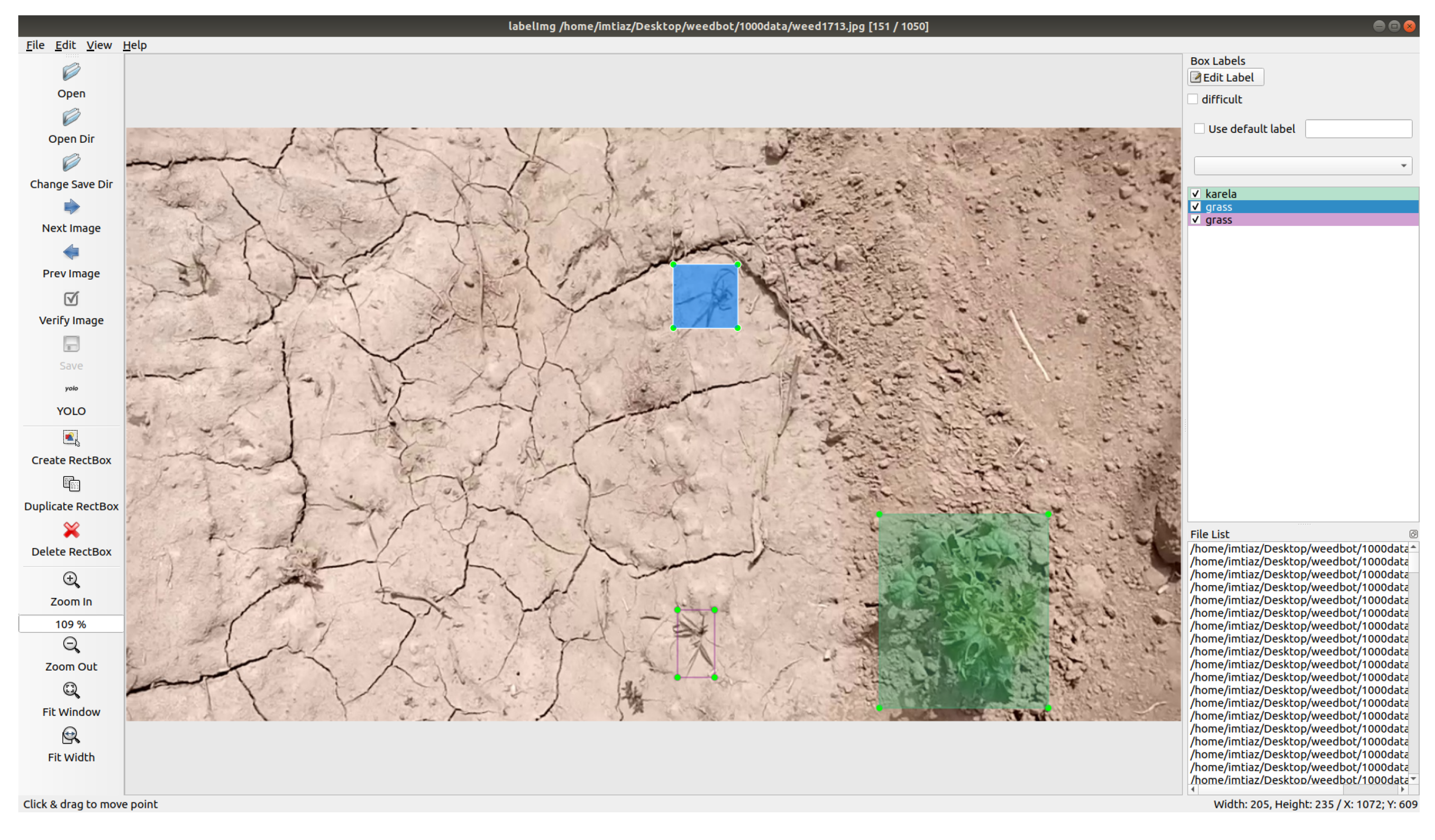
To obtain the best possible quality data extracted from the videos, noisy and blurry frames were manually removed during data cleaning. Effective data cleaning can increase both the efficiency of inferring models and their accuracy [42]. After removing noisy images from the 12,000 frames, the remaining data were 9000. The dataset obtained after preprocessing is annotated using LabelImg. It is an open-source tool for graphical image annotation that creates boxes around objects and labels them. In order to annotate an image, the image is loaded. The total number of classes is identified, which in our case is 7. After the image is loaded, the user draws a rectangular box around the images and assigns a label to it. After drawing rectangular boxes and labeling each object in the image, a text file is saved. This text file contains a bounding box and class name for every bounding box. Figure 5 shows a sample of an annotated image.

3.3. Model Development

In this study, a deep learning-based weed detection model is selected by comparing two single-stage object detection models. The performance of the selected DL models, integrated with different feature extractors, is analyzed on the images obtained after preprocessing. The total dataset consisted of 9000 images of which 1500 were chosen at random as the test set, 1500 for validation, and the remaining 6000 were used for training, respectively.

Object detection modeling is accomplished by combining localization and classification. Finding the precise location of one or more items in an image and drawing a bounding box around them is the process of localization. Image classification is the process of giving an object a label or class. Previously, object detection was performed in two stages, making the detection process difficult. In two-stage object detection, regions of interest (RoIs) were classified and regressed in two different stages. However, with recent advancements, a single-stage detector instantly classifies and regresses the anchor boxes by eliminating the RoI extraction step. YOLO5, a one-stage object detection model, is used in this study. The performance of YOLOv5 in detection and classification is then compared to that of another one-stage object detection model, SSD-Resnet. To perform real-time object detection, YOLOv5 required the least amount of inference time. Therefore, it is a suitable model for the development of a lightweight weed detection system to be mounted on a laser-based weeding robot. The section that follows provides an overview of the YOLOv5 working mechanism and its suitability for detecting and classifying weeds and crops in real-time complex agricultural environments.

3.4. YOLOv5 Network

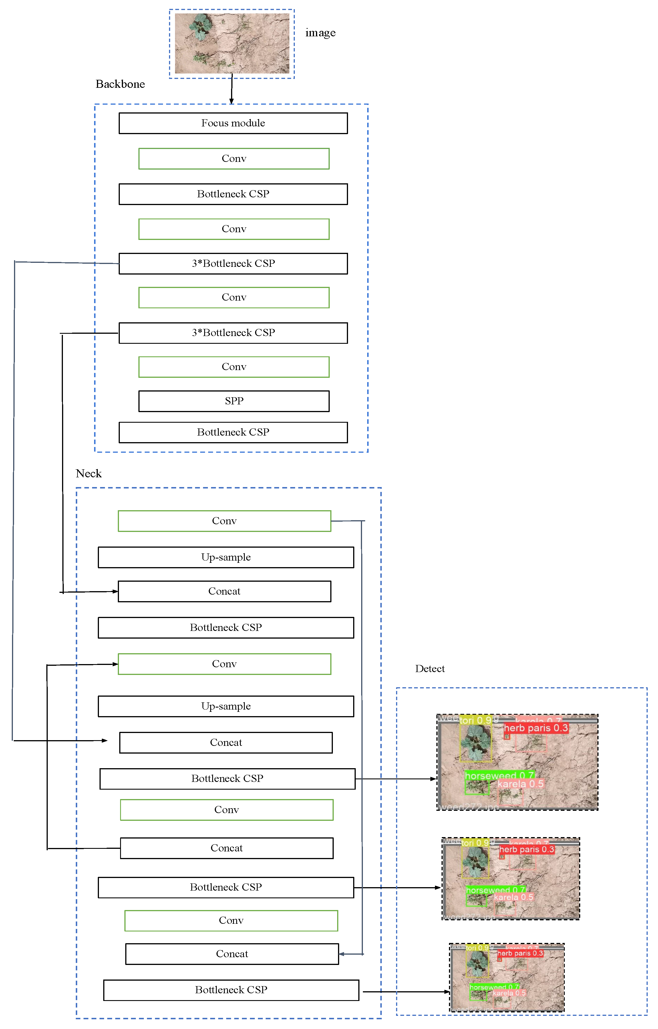
The backbone network, neck network, and detect network are the three main components of YOLO5s framework. These networks included the Focus module, the CBL module, the CSP module, the SPP module, the Concat module, and the Upsample module. Figure 6 depicts the network structure of the YOLO V5s. The YOLO5 network model has a high detection accuracy and a high inference rate, with the fastest detection rate of up to 140 frames per second. The size of the YOLOv5 pre-trained weight is 90% smaller than the size of the YOLOv4 pre-trained weight, indicating that the YOLOv5 model is suitable for deployment to embedded devices for real-time detection. The PyTorch framework is accessible and easy to train the dataset with compared to the Darknet framework used in YOLO V4. Other performance improvement features of YOLO v5 include easy integration of computer vision technologies, quick model training, and easy environment configuration. YOLO5s, YOLO5m, YOLO5l, and YOLOv5x are the four architectures that make up the YOLO5 architecture, respectively. The distinctive features of YOLO5 architectures are the depth multiplier control model and the size of the convolution cores. Both YOLO5s and YOLO5l have depth multiples of 0.33 and 1, respectively. The recognition model had to adhere to strict real-time performance and lightweight requirements because the study’s focus was the detection and classification of seven different objects, of which there were three crop types and four weed species. Therefore, after careful examination and analysis of the accuracy, efficiency, and size of the detection model, the weed detection system for precise and real-time laser-based killing in fields was made by using the YOLO5s model [43].

3.5. SSD-ResNet Network

The working mechanism of the SSD-ResNet model is nearly the same as YOLO5. It creates a set of bounding boxes with a specified size and predicts a confidence score of the object’s category within the bounding boxes. The SSD design combines the pyramidal feature hierarchy structure with the CNN model of ResNet network as a backbone structure to predict many scales of feature maps with various resolutions [44].

3.6. Performance Metrics

We used popular metrics, such as precision, recall, average precision, and mean average precision, to assess the performance of object detection models YOLOv5s and SSD-ResNet. These metrics are as follows:

3.6.1. Precision

Precision is a standard metric to evaluate performance of a model. It is defined as the ratio of values accurately predicted as positive to all values predicted as positive. A higher precision indicates a lower rate of false positives [45]. The formula for precision is given in Equation (1) [46]:

$$P=\frac{TP}{TP+FP},$$

(1)

where $TP$ and $FP$ refer to true positives and false positives, respectively.

3.6.2. Recall

Recall is calculated as the ratio of values correctly predicted as positive to all positive samples in the dataset. It determines the ability of a model to predict a positive as shown in Equation (2) [45].

$$R=\frac{TP}{TP+FN},$$

(2)

where $TP$ and $FN$ refer to true positives and false negatives, respectively.

3.6.3. Average Precision (AP) and Mean Average Precision mAP

AP (average precision) is calculated by averaging the precision for recall value over 0 to 1. In other words, AP is the area under curve for a precision–recall curve [45]. The equation for AP is given in Equation (3) [46]:

$$A{P}_i={\int }_0^{1}P\left(R\right)d\left(R\right)$$

(3)

where P and R denote precision and recall, respectively. Finding the mean of AP for all classes gives us the mAP Equation (4) [46]:

$$mAP=\frac{1}{cls}\sum _{i=cls}AP\left(i\right)$$

(4)

where cls represents the number of classes.

4. Results

4.1. Model Training Setup

The weights of Yolov5s, which is the most lightweight model in the YOLOV5 family, were used as the initial weights. The model was trained for 15 epochs. Because of the memory constraints, the batch size was set to 4. The stochastic gradient descent (SGD) was used for optimization. The learning rate $lr$ was set to $0.01$.

The training was performed using a computer system with a 4GB 5124 Volta GPU desktop computer graphics card with 4 GB of GPU, and 32 GB of RAM was used. The model was trained on the Linux operating system using the Pytorch framework. The model with the mAP value was saved and chosen to be employed on the real-time laser weeding robot. To reduce the computational complexity of the training, each input image was scaled to 640 × 640.

4.2. Training Results

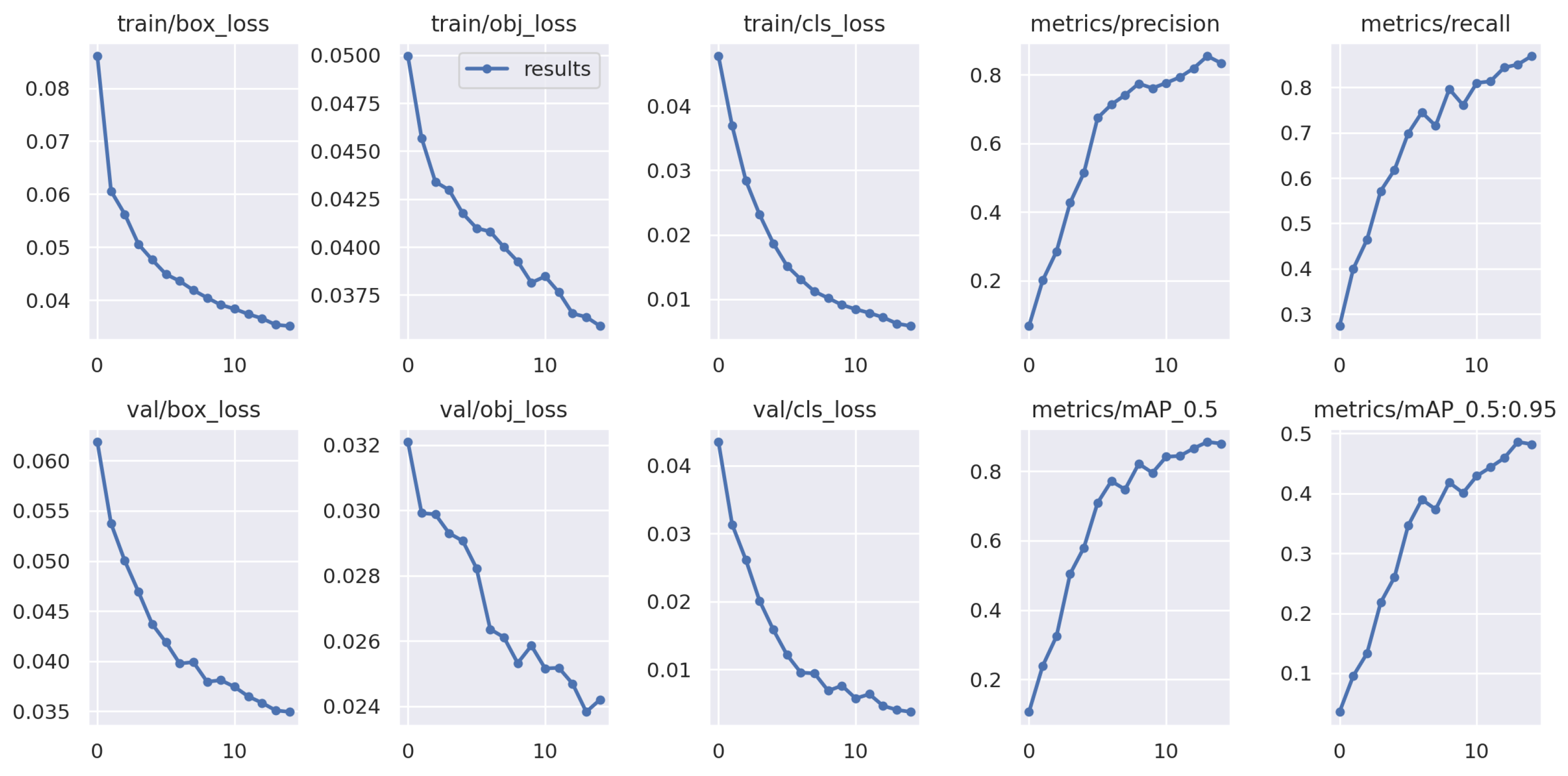
The different loss functions and evaluation metrics for the training of the YOLOv5s can be seen in Figure 7. The curves in the figure illustrate three distinct forms of loss functions: box loss, object loss, and classification loss. The predictive bounding box coverage of the target object is measured in terms of box loss. Essentially, abjectness measures how likely it is that a specific object will be found in a particular region of interest. High objectivity shows whether an object is present in a certain image window. The discrepancy between a prediction box object’s actual class and the anticipated class is known as classification loss. It is evident from the figure that the model’s performance gets better over every epoch. Moreover, we can see that precision and recall for both training and testing keep increasing, which suggests that the model is not over-fitting. Furthermore, we can see that near the 15 epochs, the model training and testing loss are converging.

4.3. Test Results

Better training results do not always imply that the model has learned more effectively, as sometimes, over-fitted models have high training accuracy. As a result, the test dataset is used to evaluate the model on previously unseen data.

Table 1. Validation metrics for YOLOv5.

mAP@IOU 0.5	mAP@IOU 0.95	Precision	Recall
0.88	0.48	0.83	0.86

shows the various validation metrics for the proposed YOLO5 model.

Prediction of the model on a test dataset can be seen in Figure 8. Prediction boxes represent each of the three crop types and four weed species, and the network’s final output includes the probability of each category’s inclusion as well as their locations.

Confusion Matrix

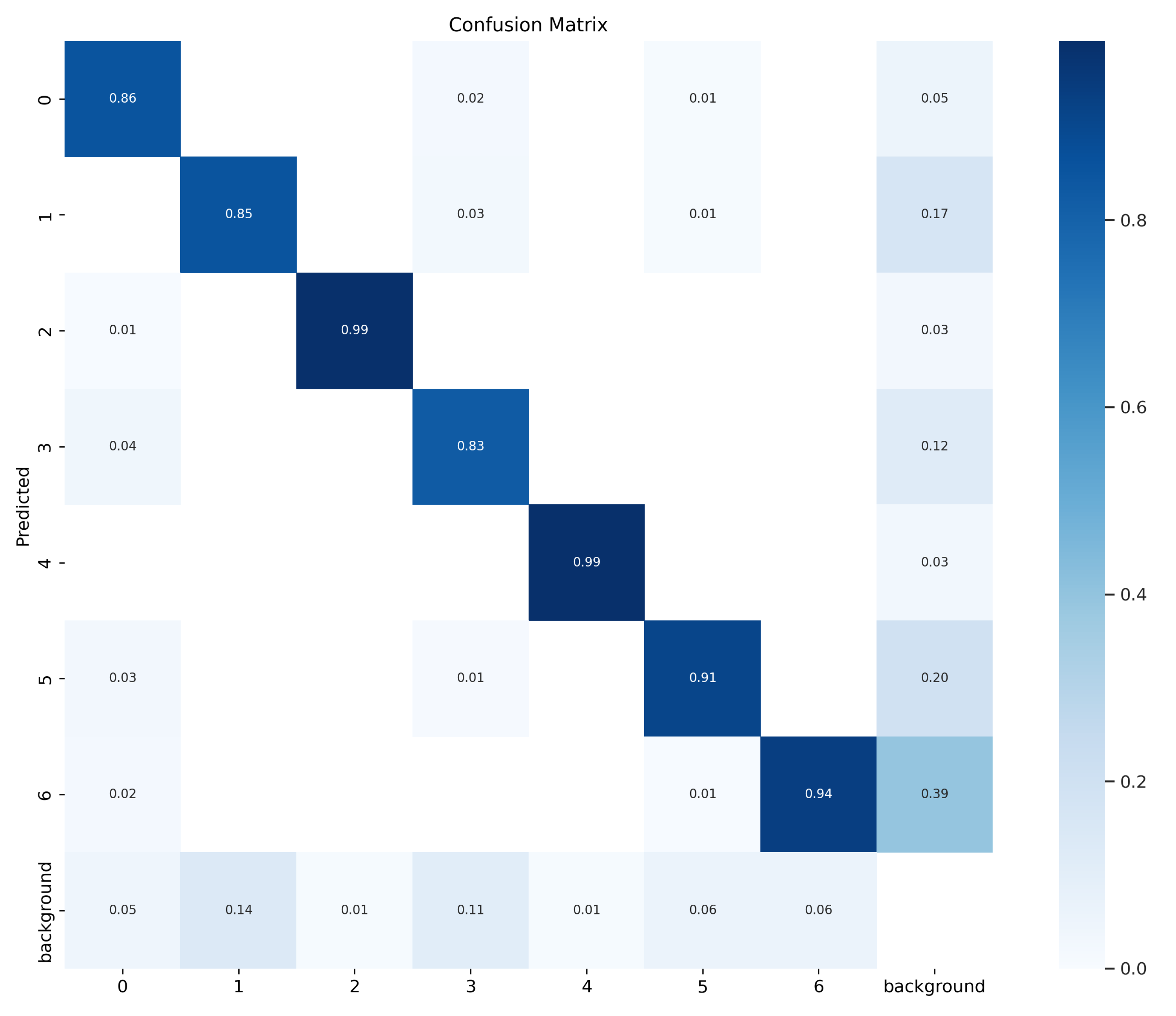
After testing the YOLO5 model with the collected dataset, a confusion matrix (shown in Figure 9) was created, and the results were evaluated based on the accuracy of classification for four weed species and three crop types. At the time of the annotation, all 7 classes, including crops and weeds, were assigned code numbers. Herb Paris is coded as 0, bitter gourd is coded as 1, small weed is coded as 2, grass class is coded as 3, sponge gourd is coded as 4, horseweed is coded as 5, and okra is coded as 6. The results of the matrix revealed that the model performed exceptionally well for object localization and classification, with the highest prediction accuracy for sponge gourd and small weed at 99%, okra at 94%, and horseweed at 91%. Low prediction accuracy rates were obtained for Herb Paris (86%), bitter gourd (85%) and grass (83%). In numerous instances, the model incorrectly identified grass as bitter gourd because of its similar physical features, such as leaf size, shape, and color. Figure 9 depicts a confusion matrix of a single validation batch.

4.4. Comparison of the Models, YOLOv5 and SSD-ResNet

For evaluating the performance of YOLO5, another one-stage object detection model, SSD-ResNet is trained to compare the precision score and inference time. In the SSD-ResNet model, the performance slightly declines when the object size is very small. This model seems to work well in identifying large objects, but its performance and accuracy are somewhat compromised while detecting very small objects. YOLO5, on the other hand, is an excellent choice for detecting small objects. As in our study, the object to be detected is a mixture of weeds and crops grown in the same field. Weeds are typically very small in size in their early stages; they should be detected and killed before they grow into large bushes, as they consume all of the crop nutrients. In comparison to the SSD-ResNet model, which performed at a rate of 30 frames per second, YOLO5 accurately and quickly detected small weeds and crops from the image at a rate of 40 frames per second. The outperformance of the YOLO5 model in detecting weeds and crops made it suitable for detecting and classifying weeds and crops within fields. A comparison of performance charts in terms of mAP values and inference time is shown in

Table 2. Performance comparison of YOLOv5 and SSD-ResNet.

Model	mAP@IOU 0.5	mAP@IOU 0.95	FPS (Frame per Second)
YOLO v5	0.88	0.48	40
SSD	0.53	0.25	30

. Additionally, the total loss function curve for the SSD-ResNet model after 15 training epochs is shown in Figure 10.

4.5. Deployment on the Standalone Embedded Device

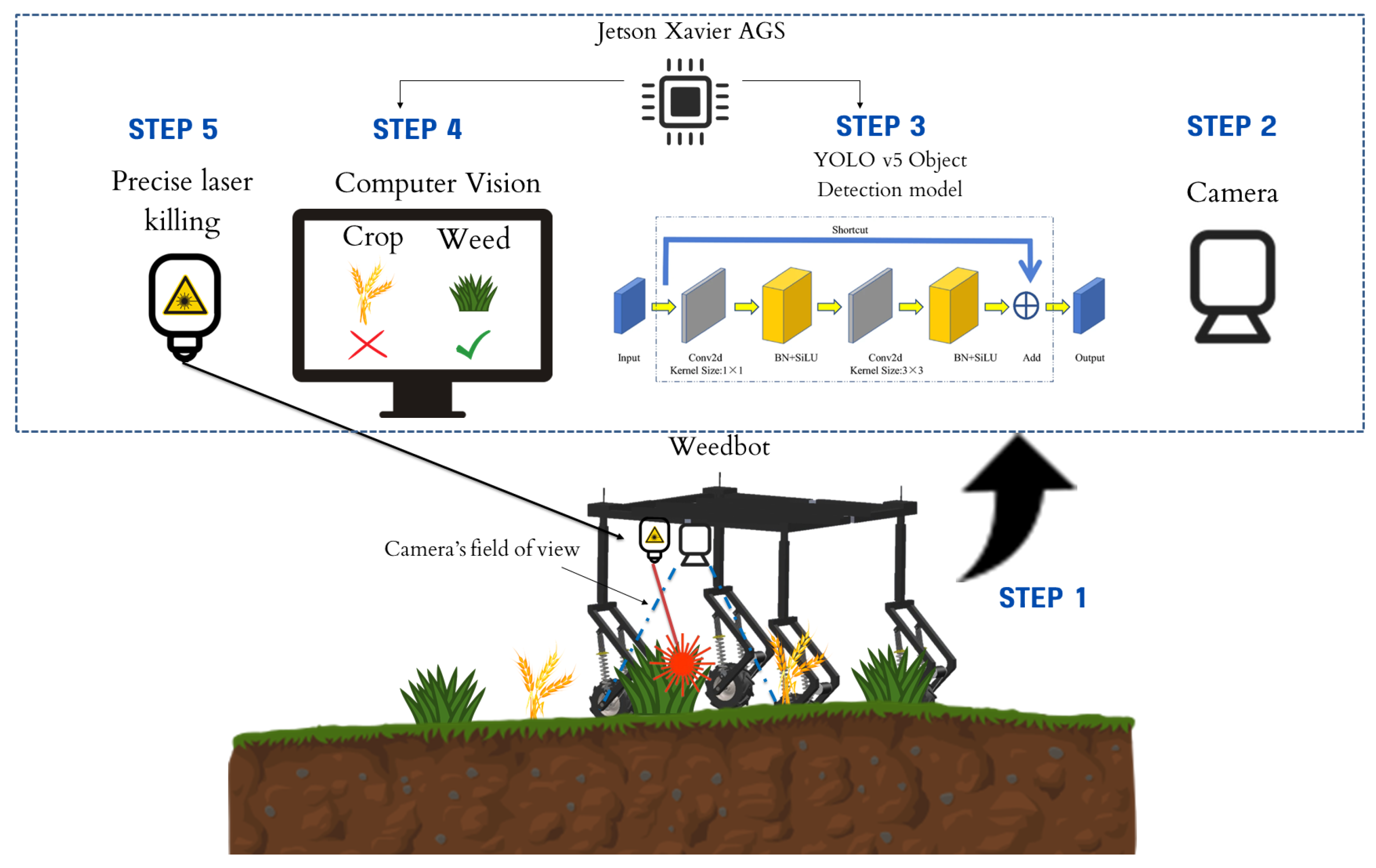
In order to make the detection system robust, the trained YOLO5 model was further tested on a standalone embedded device, the Nvidia Xavier AGX. NVidia Jetson devices are embedded AI computing platforms that provide high-performance, low-power computing support for deep learning models. The trained YOLO5 model was tested and deployed on an Nvidia Xavier AGX (the latest module in the series), which has a 4GB 5124 Volta GPU with Tensorboards. The model was running at 27 FPS (frames per second), which can be used for real-time applications. Figure 11 shows the working mechanism of a real-time, laser-based weed detection system.

5. Conclusions and Future Work

The study aimed to build, analyze, and evaluate a deep learning model for providing machine vision to autonomous weeding robots. To develop a weed detection system, the deep learning-based single-stage object detection model YOLO5 is used. The model is then compared with another single-shot detector SSD-ResNet to assess its performance.

The dataset was created by visiting multiple Agri farm fields in different parts of Pakistan. The videos yielded a total of 12,000 frames (images). Following the removal of noisy images, the remaining 9000 images contained three different crops and four weed species. A total of 1500 photos were selected at random as the test set, with the remaining 7500 serving as the test set. The training was set for 15 epochs. YOLO5 accurately and quickly detected weeds and crops in images at a rate of 40 frames per second with a detection speed of 0.02 s per image and mAP [email protected] of 0.88. On the other hand, SSD ResNet detected weeds and crops in the images at a rate of 30 FPS with a speed of 0.046 s and a mAP [email protected] of 0.53. The superior performance of the YOLO5 model makes it a suitable DL model for detecting and classifying weeds and crops within fields. In order to make the detection system robust, the trained YOLO5 model was further tested on a standalone embedded device, the Nvidia Xavier AGX. Based on the performance of the developed weed detection system, it can be commercially employed on an autonomous laser weeding vehicle for real-time site-specific weed management without causing crop damage.

The future work will focus on collecting more data for the given crops and weed species, as the accuracy for Herb Paris, bitter gourd, and the grass was relatively low. Furthermore, data will be collected for more crops and weed species, as, being an agricultural country, Pakistan produces a wide variety of crops. Therefore, collecting data for a wider variety of crops and weed species could help improve the accuracy and effectiveness of object detection models for agricultural applications in Pakistan.

References

1. Distribution of Gross Domestic Product (GDP) across Economics Sector 2020. 15 February 2022. Available online: https://www.statista.com/statistics/383256/pakistan-gdp-distribution-across-economic-sectors/ (accessed on 19 August 2022).
2. Ali, H.H.; Peerzada, A.M.; Hanif, Z.; Hashim, S.; Chauhan, B.S. Weed management using crop competition in Pakistan: A review. Crop Prot. 2017, 95, 22–30. [Google Scholar] [CrossRef]
3. Fennimore, S.A.; Slaughter, D.C.; Siemens, M.C.; Leon, R.G.; Saber, M.N. Technology for automation of weed control in specialty crops. Weed Technol. 2016, 30, 823–837. [Google Scholar] [CrossRef]
4. Chauhan, B.S. Grand challenges in weed management. Front. Agron. 2020, 1, 3. [Google Scholar] [CrossRef]
5. Weeds Cause Losses Amounting to Rs65b Annually. 20 July 2017. Available online: https://tribune.com.pk/story/1461870/weeds-cause-losses-amounting-rs65b-annually (accessed on 19 August 2022).
6. Bai, S.H.; Ogbourne, S.M. Glyphosate: Environmental contamination, toxicity and potential risks to human health via food contamination. Environ. Sci. Pollut. Res. 2016, 23, 18988–190017. [Google Scholar] [CrossRef]
7. Chauhan, B.S. Weed ecology and weed management strategies for dry-seeded rice in Asia. Weed Technol. 2012, 26, 1–13. [Google Scholar] [CrossRef]
8. Bronson, K. Smart Farming: Including Rights Holders for Responsible Agricultural Innovation. Technol. Innov. Manag. Rev. 2018, 8, 7–14. [Google Scholar] [CrossRef] [Green Version]
9. Dammer, K.H. Real-time variable-rate herbicide application for weed control in carrots. Weed Res. 2016, 56, 237–246. [Google Scholar] [CrossRef]
10. Dar, M.A.; Kaushik, G.; Chiu, J.F.V. Pollution status and biodegradation of organophosphate pesticides in the environment. In Abatement of Environmental Pollutants; Elsevier: Amsterdam, The Netherlands, 2020; pp. 25–66. [Google Scholar]
11. Westwood, J.H.; Charudattan, R.; Duke, S.O.; Fennimore, S.A.; Marrone, P.; Slaughter, D.C.; Swanton, C.; Zollinger, R. Weed management in 2050: Perspectives on the future of weed science. Weed Sci. 2018, 66, 275–285. [Google Scholar] [CrossRef] [Green Version]
12. Mhlanga, D. Artificial intelligence in the industry 4.0, and its impact on poverty, innovation, infrastructure development, and the sustainable development goals: Lessons from emerging economies? Sustainability 2021, 13, 5788. [Google Scholar] [CrossRef]
13. Ali, M.M.; Bachik, N.A.; Muhadi, N.A.; Yusof, T.N.T.; Gomes, C. Non-destructive techniques of detecting plant diseases: A review. Physiol. Mol. Plant Pathol. 2008, 108, 101426. [Google Scholar] [CrossRef]
14. Mavridou, E.; Vrochidou, E.; Papakostas, G.A.; Pachidis, T.; Kaburlasos, V.G. Machine vision systems in precision agriculture for crop farming. J. Imaging 2019, 5, 89. [Google Scholar] [CrossRef] [Green Version]
15. Eli-Chukwu, N.C. Applications of artificial intelligence in agriculture: A review. Eng. Technol. Appl. Sci. Res. 2019, 9, 4377–4383. [Google Scholar] [CrossRef]
16. Di Cicco, M.; Potena, C.; Grisetti, G.; Pretto, A. Automatic model based dataset generation for fast and accurate crop and weeds detection. In Proceedings of the 2017 IEEE/RSJ International Conference on Intelligent Robots and Systems (IROS), Vancouver, BC, Canada, 24–28 September 2017; pp. 5188–5195. [Google Scholar]
17. Hasan, A.M.; Sohel, F.; Diepeveen, D.; Laga, H.; Jones, M.G. A survey of deep learning techniques for weed detection from images. Comput. Electron. Agric. 2018, 184, 106067. [Google Scholar] [CrossRef]
18. Firmansyah, E.; Suparyanto, T.; Hidayat, A.A.; Pardamean, B. Real-time Weed Identification Using Machine Learning and Image Processing in Oil Palm Plantations. In IOP Conference Series: Earth and Environmental Science; IOP Publishing: Bristol, UK, 2022. [Google Scholar]
19. Pushpanathan, K.; Hanafi, M.; Mashohor, S.; Fazlil Ilahi, W.F. Machine learning in medicinal plants recognition. Artif. Intell. Rev. 2021, 30, 823–837. [Google Scholar] [CrossRef]
20. Cope, J.S.; Corney, D.; Clark, J.Y.; Remagnino, P.; Wilkin, P. Plant species identification using digital morphometrics: A review. Expert Syst. Appl. 2012, 39, 7562–7573. [Google Scholar] [CrossRef]
21. Le-Khac, P.H.; Healy, G.; Smeaton, A.F. Contrastive representation learning: A framework and review. J. Framew. Rev. 2020, 10, 193907–193934. [Google Scholar] [CrossRef]
22. Lee, S.H.; Chan, C.S.; Mayo, S.J.; Remagnino, P. How deep learning extracts and learns leaf features for plant classification. Pattern Recognit. 2017, 71, 1–13. [Google Scholar] [CrossRef] [Green Version]
23. Chang, J.; Sitzmann, V.; Dun, X.; Heidrich, W.; Wetzstein, G. Hybrid optical-electronic convolutional neural networks with optimized diffractive optics for image classification. Sci. Rep. 2018, 8, 7562–7573. [Google Scholar] [CrossRef] [Green Version]
24. Sultana, F.; Sufian, A.; Dutta, P. A review of object detection models based on convolutional neural network. In Intelligent Computing: Image Processing Based Applications; Springer: Berlin, Germany, 2020; pp. 1–16. [Google Scholar]
25. Chen, W.; Huang, H.; Peng, S.; Zhou, C.; Zhang, C. YOLO-face: A real-time face detector. Vis. Comput. 2021, 37, 805–813. [Google Scholar] [CrossRef]
26. Tan, Y.; Cai, R.; Li, J.; Chen, P.; Wang, M. Automatic detection of sewer defects based on improved you only look once algorithm. Autom. Constr. 2021, 131, 103912. [Google Scholar] [CrossRef]
27. Liu, W.; Anguelov, D.; Erhan, D.; Szegedy, C.; Reed, S.; Fu, C.Y.; Berg, A.C. Ssd: Single shot multibox detector. In European conference on Computer Vision; Springer: Cham, Switzerland, 2016; pp. 21–37. [Google Scholar]
28. Deploy AI-Powered Autonomous Machines at Scale. Available online: https://www.nvidia.com/en-us/autonomous-machines/embedded-systems/jetson-agx-xavier/ (accessed on 31 October 2022).
29. Sethia, G.; Guragol, H.K.S.; Sandhya, S.; Shruthi, J.; Rashmi, N.; Sairam, H.V. Automated Computer Vision based Weed Removal Bot. In Proceedings of the 2020 IEEE International Conference on Electronics, Computing and Communication Technologies (CONECCT), Bangalore, India, 2–4 July 2020. [Google Scholar]
30. Smith, L.N.; Byrne, A.; Hansen, M.F.; Zhang, W.; Smith, M.L. Weed classification in grasslands using convolutional neural networks. Appl. Mach. Learn. 2019, 11139, 334–344. [Google Scholar]
31. Bakhshipour, A.; Jafari, A. Evaluation of support vector machine and artificial neural networks in weed detection using shape features. Comput. Electron. Agric. 2018, 145, 153–160. [Google Scholar] [CrossRef]
32. Alam, M.; Alam, M.S.; Roman, M.; Tufail, M.; Khan, M.U.; Khan, M.T. Real-time machine-learning based crop/weed detection and classification for variable-rate spraying in precision agriculture. In Proceedings of the 2020 7th International Conference on Electrical and Electronics Engineering (ICEEE), Antalya, Turkey, 14–16 April 2020. [Google Scholar]
33. Quan, L.; Feng, H.; Lv, Y.; Wang, Q.; Zhang, C.; Liu, J.; Yuan, Z. Maize seedling detection under different growth stages and complex field environments based on an improved Faster R–CNN. Biosyst. Eng. 2019, 184, 1–23. [Google Scholar] [CrossRef]
34. Wang, Z.; Liu, J. A review of object detection based on convolutional neural network. In Proceedings of the 2017 36th Chinese Control Conference (CCC), Dalian, China, 26–28 July 2017; pp. 11104–11109. [Google Scholar]
35. Jiang, P.; Ergu, D.; Liu, F.; Cai, Y.; Ma, B. A Review of Yolo algorithm developments. Procedia Comput. Sci. 2022, 199, 1066–1073. [Google Scholar] [CrossRef]
36. Abdulsalam, M.; Aouf, N. Deep weed detector/classifier network for precision agriculture. In Proceedings of the 2020 28th Mediterranean Conference on Control and Automation (MED), Saint-Rapha, France, 15–18 September 2020. [Google Scholar]
37. Sanchez, P.R.; Zhang, H.; Ho, S.S.; De Padua, E. Comparison of one-stage object detection models for weed detection in mulched onions. In Proceedings of the 2021 IEEE International Conference on Imaging Systems and Techniques (IST), Kaohsiung, Taiwan, 24–26 August 2021. [Google Scholar]
38. Jin, X.; Sun, Y.; Che, J.; Bagavathiannan, M.; Yu, J.; Chen, Y. A novel deep learning-based method for detection of weeds in vegetables. Pest Manag. Sci. 2022, 78, 1861–1869. [Google Scholar] [CrossRef]
39. Veeranampalayam Sivakumar, A.N.; Li, J.; Scott, S.; Psota, E.; Jhala, A.J.; Luck, J.D.; Shi, Y. Comparison of object detection and patch-based classification deep learning models on mid-to late-season weed detection in UAV imagery. Pest Manag. Sci. 2022, 78, 2136. [Google Scholar] [CrossRef]
40. Olaniyi, O.M.; Daniya, E.; Abdullahi, I.M.; Bala, J.A.; Olanrewaju, E. Weed recognition system for low-land rice precision farming using deep learning approach. In Proceedings of the International Conference on Artificial Intelligence & Industrial Applications, Meknes, Morocco, 19–20 March 2020; pp. 385–402. [Google Scholar]
41. YOLOv5: The Friendliest AI Architecture You’ll Ever Use. 2022. Available online: https://ultralytics.com/yolov5 (accessed on 22 November 2022).
42. Zhou, L.; Pan, S.; Wang, J.; Vasilakos, A.V. Machine learning on big data: Opportunities and challenges. Neurocomputing 2017, 237, 350–361. [Google Scholar] [CrossRef] [Green Version]
43. Xu, R.; Lin, H.; Lu, K.; Cao, L.; Liu, Y. A forest fire detection system based on ensemble learning. Forests 2017, 12, 217. [Google Scholar] [CrossRef]
44. Lu, X.; Kang, X.; Nishide, S.; Ren, F. Object detection based on SSD-Ren. In Proceedings of the 2019 IEEE 6th International Conference on Cloud Computing and Intelligence Systems (CCIS), Singapore, 19–21 December 2019. [Google Scholar]
45. Confusion Matrix, Accuracy, Precision, Recall, F1 Score. 2019. Available online: https://medium.com/analytics-vidhya/confusion-matrix-accuracy-precision-recall-f1-score-ade299cf63cd (accessed on 10 December 2019).
46. Padilla, R.; Netto, S.L.; Da Silva, E.A. A survey on performance metrics for object-detection algorithms. In Proceedings of the 2020 International Conference on Systems, Signals and Image Processing (IWSSIP), Niteroi, Brazil, 1–3 July 2020. [Google Scholar]
Figure 1. Workflow for the development of the weed detection mechanism.
Applsci 13 03997 g001
Figure 2. Visuals of various crops collected in the dataset. Each column contains different sample images of the crops in the collected data. Column (a) represents sponge gourd, (b) okra, and (c) bitter gourd, respectively.
Applsci 13 03997 g002
Figure 3. Visuals of the commonly occurred weeds in the fields. Multiple images of each weed species are arranged in columns.
Applsci 13 03997 g003
Figure 4. The dataset is represented in a bar graph, where the frequency of each class is depicted. The graph reveals that okra has the most number of samples, while smallweed and sponge gourd have a lower count of instances.
Applsci 13 03997 g004
Figure 5. An annotated sample image using an open source tool LabelImg.
Applsci 13 03997 g005
Figure 6. Architecture of the single-shot YOLOv5s model showing its three main components, i.e., the backbone network, neck network, and detect network.
Applsci 13 03997 g006
Figure 7. Distinct forms of loss functions and performance metrics, that include boxloss, objectloss, precision, recall and mAP.
Applsci 13 03997 g007
Figure 8. The figure depicts the bounding boxes generated by the YOLOv5s model, as well as the class label and confidence value. Bitter gourd coded as 1, small weed coded as 2, grass class coded as 3, sponge gourd coded as 4, horseweed coded as 5, and okra coded as 6. Okra with class label 6 received a confidence score of 0.9 on the provided data, indicating that the model correctly predicted the okra class with 90% confidence.
Applsci 13 03997 g008
Figure 9. Confusion matrix for YOLOV5 on validation data.
Applsci 13 03997 g009
Figure 10. The total loss function curve for the SSD-RestNet model.
Applsci 13 03997 g010
Figure 11. Functioning of a real-time, laser-based weed detection system.
Applsci 13 03997 g011