Article

Modelling the Wind Speed Using Exponentiated Weibull Distribution: Case Study of Poprad-Tatry, Slovakia

by
Ivana Pobočíková
1,*,
Mária Michalková
1,
Zuzana Sedliačková
1 and
Daniela Jurášová
2
1
Department of Applied Mathematics, Faculty of Mechanical Engineering, University of Žilina, Univerzitná 8215/1, 010 16 Žilina, Slovakia
2
Department of Building Engineering and Urban Planning, Faculty of Civil Engineering, University of Žilina, Univerzitná 8215/1, 010 16 Žilina, Slovakia
*
Author to whom correspondence should be addressed.
Appl. Sci. 2023, 13(6), 4031; https://doi.org/10.3390/app13064031
Submission received: 20 February 2023 / Revised: 13 March 2023 / Accepted: 17 March 2023 / Published: 22 March 2023
(This article belongs to the Section Environmental Sciences)

Abstract

:
In the paper, we statistically analysed data on the average hourly wind speed obtained from the meteorological station Poprad (located at the Poprad-Tatry airport, the Prešov region, Northern Slovakia) for the period 2005–2021. High altitude and rough mountainous terrain influence the weather conditions considerably and are a source of occasional weather risks. Finding an appropriate wind speed distribution for modelling the wind speed data is therefore important to determine the wind profile at this particular location. In addition to the commonly used two- and three-parameter Weibull distribution, a more flexible exponentiated Weibull (EW) distribution was applied to model the wind speed. Based on the results of the goodness-of-fit criteria (the Kolmogorov–Smirnov test, the Anderson–Darling test, Akaike’s and Bayesian information criteria, the root mean square error, and the coefficient of determination), the EW distribution obtained a significantly better fit to seasonal and monthly wind speed data, especially around the peaks of the data. The EW distribution also proved to be a good model for data with high positive skewness. Therefore, we can recommend the EW distribution as a flexible distribution for modelling a dataset with extremely strong winds or outliers in the direction of the right tail. Alongside the wind speed analysis, we also provided the wind direction analysis, finding out that the most prevailing direction was west (W)—with an occurrence rate of 34.99%, and a mean wind speed of 3.91 m/s, whereas the northern (N) direction featured the lowest occurrence rate of only 4.45% and the mean wind speed of 1.99 m/s.

1. Introduction

The wind speed is extremely variable; at a given location it varies with time and height while also depending on the shape and roughness of the terrain (surrounding landscape, vegetation, and structures). The wind speed decreases with a rougher surface, but it can accelerate on steep hills, reaching its maximum at the crest and then splitting into zones of turbulent air flow. Its fluctuating nature requires appropriate means for its description, and right here the probability distributions can provide a useful tool in modelling the wind speed. Wind speed modelling via probability distributions, which is based on long-term observations, is relatively stable and based on long-term statistical characteristics of wind [1,2]. Because strong winds are known to be rare, whilst mild and fresh winds are more common, the probability distributions more suitable for wind speed modelling are those skewed to the right. The two-parameter Weibull distribution is often presented as the first choice for modelling many wind sites since it can provide a good agreement with the experimental data [3]. This probability distribution has many advantages, such as a simple form, high flexibility, the probability density function and the cumulative distribution function are described in a closed form, and a relatively simple estimation of the parameters. It was first introduced by the Swedish scientist Walodi Weibull (1887–1979), who used it in the theory of reliability. The Weibull distribution appears to be a powerful tool for statistical analysis of data in many areas, such as engineering, materials science, quality, physics, medicine, meteorology, and hydrology. The use of the Weibull distribution to describe the wind speed has a long history. This distribution was first applied to wind speed data by Davenport in [4]. Since then, it has been successfully used for modelling the wind speed in many sites, for example, in India [5], Pakistan [6,7], South Korea [8], West Africa [9], U.S.A. [10], Cook Islands [11], Palestine [12], Iraq [13], Nigeria [14], United Kingdom [15], Austria [16], Slovakia [17], and many more. Therefore, the Weibull distribution is commonly used as a wind speed distribution and is implemented in many commercial programs [18]. However, the two-parameter Weibull distribution is not universal and it does not suit all the existing wind regimes [19]. As previous studies have shown, the two-parameter Weibull distribution is less effective in fitting low wind speeds, especially when the probability of null wind is significant—null wind speed data needs to be removed before fitting, making it impossible to characterise some of the existing wind regimes [18,20]. As an alternative to the two-parameter Weibull distribution, the three-parameter Weibull distribution has also been used in some studies, and it has been found to provide a greater flexibility than the classical two-parameter Weibull function [21,22]. It proved to better fit the wind speed (compared to the two-parameter Weibull function) when there is a higher frequency of lower values of wind speed, including null wind [18]. This has motivated authors to successfully apply other known probability distributions, for example, Extreme Value [23], Gamma [24], Gumbel [25], Nakagami [26], Birnbaum–Saunders [27], Wakeby and Kappa [28], Lindley [29], and many more. Furthermore, it propelled many authors to search for more flexible and better fitting probability distributions using generalizations of classical probability distributions. Several methods to improve the flexibility by adding one or more parameters to the distributions have been proposed and such generalizations have been made through different approaches [30]: the transformation method [31,32], the composition of two or more distributions, the compounding of distributions, and the mixture of classical distributions [33,34,35,36,37].
In this study, we dealt with the exponentiated Weibull distribution as an alternative to the widely used wind speed distributions, namely the two-parameter and three-parameter Weibull distributions. An exponentiated probability distribution was created by exponentiation of the classical distribution. Specifically, the cumulative distribution function of a probability distribution was raised to an additional parameter. It was studied in [38] where authors investigated several exponentiated probability distributions in detail. Exponentiated Weibull distribution as a generalization of the Weibull distribution was introduced by Mudholkar a Srivastava in [39]. Its properties were studied in [40,41,42,43,44,45,46]. This distribution has been commonly used for modelling data in various fields, such as reliability, finance, medicine, and environmental studies [47,48].
Considering the limitation of the two-parameter and three-parameter Weibull distributions in modelling the wind speed, here, it was investigated whether the exponentiated Weibull distribution is sufficiently flexible and adaptable to accommodate different shapes of the wind speed data. The number of papers dedicated to application of the exponentiated Weibull distribution on fitting the wind speed data is rather limited. Shittu and Adepoju in [49] used the two-parameter Weibull and the exponentiated Weibull distribution, respectively, to model wind speeds in Southwestern Nigeria using long-term observations covering the period of years 1992–2012. Based on the values of the Akaike’s information criterion, they demonstrated a much better fit of the exponentiated Weibull distribution as compared to the performance of the Weibull distribution. Gül Akgül and Şenoğlu in [50] modelled the wind speed in six stations located on the Aegean coast, Turkey. They compared nine different probability distributions, namely the Rayleigh, the inverse Weibull, the Burr Type III, the Extreme value, the Gamma, the inverse Gamma, the Marshall–Olkin extended Lindley, the generalized Extreme value, and the exponentiated Weibull distribution, since these distributions represent suitable alternatives to the Weibull distribution in modelling the wind speed. According to the values of the model evaluation criteria (the root mean square error, the coefficient of determination, the Akaike’s information criterion, the Bayesian information criterion, and the Kolmogorov–Smirnov test statistic), the exponentiated Weibull distribution outperformed the rest of the considered distributions. Both of the mentioned papers focused on modelling the wind speed in stations located in the coastal area with low altitudes. To the best of our knowledge, there has not been published a paper focusing on the application of the exponentiated Weibull distribution to model the wind speed in a location with a higher altitude, laying inland. For this purpose, the hourly wind speed data from meteorological station Poprad, located at the Poprad-Tatry airport, Northern Slovakia, was modelled by two-parameter, three-parameter, and exponentiated Weibull distributions, respectively.
The city of Poprad is the administrative, economic, and cultural centre of the region under the Tatras. With a population of 49,430 (31.12.2021), it is the second largest city in the Prešov region and the tenth largest city in Slovakia. Thanks to its location, it was given the epithet “The gateway to the High and Low Tatras”, where there are well-known centres for winter sports and summer tourism. The High Tatras are the only high mountains that are located on the territory of Slovakia and Poland and are also included in the UNESCO Biosphere Reserve. The highest peak of the High Tatras as well as of the entire Carpathians is the Gerlach peak (2654.4 m above sea level). The territory of the biosphere reserve includes two national parks, one of which is in Slovakia. The tourism sector in the Tatra Biosphere Reserve provides the main form of employment [51]. The Poprad-Tatry airport plays an important role in the local economic dependence on tourism. Weather risks and wind directly affect the safety of air transportation and the operations at the airport. Therefore, it is important to investigate and analyse the influence of the mountain environment on the course of meteorological phenomena. In this article, we examine the wind speed and direction in this location because they are important for the safety of the airport operations. Based on the long-term observations, it is possible to predict how the wind speed and direction will develop in a given location. Accurate wind speed forecasts are necessary for both short- and long-term warning planning and decision-making in these applications.
The parameters of the considered probability distributions were estimated using the maximum likelihood method (MLM) and the calculations were performed in the statistical software STATISTICA and software MATLAB R2020b. The computations carried out in the Matlab software were based on functions available in the Statistics and Machine Learning Toolbox, customized by the authors. In order to assess the goodness-of-fit (GOF) of the selected probability distributions, the commonly used GOF tests—the Kolmogorov–Smirnov (KS) test and the Anderson–Darling (AD) test—were applied. Moreover, the root mean square error (RMSE), the coefficient of determination (R2), and the information criteria—Akaike’s information criterion (AIC) and Bayesian information criterion (BIC)—were used to assess the suitability of the considered probability distributions and to compare their performances.
The rest of this article is organized as follows: in “Description of studied area”, we briefly describe the geographical conditions of the studied area of the Poprad-Tatry airport and characterise the meteorological station situated there. The section “Wind speed description and analysis” provides characteristics of the datasets along with their descriptive statistics. The section “Wind Direction Analysis” summarises the results of the analysis in the form of wind roses. In “Methods”, we give a summary of the modelled probability distributions, of the parameter estimation method, and of the GOF and model selection criteria. The section “Results and discussion” summarises and discusses the obtained results. The section “Conclusion” recapitulates our findings and provides recommendations for the application of the exponentiated Weibull distribution.

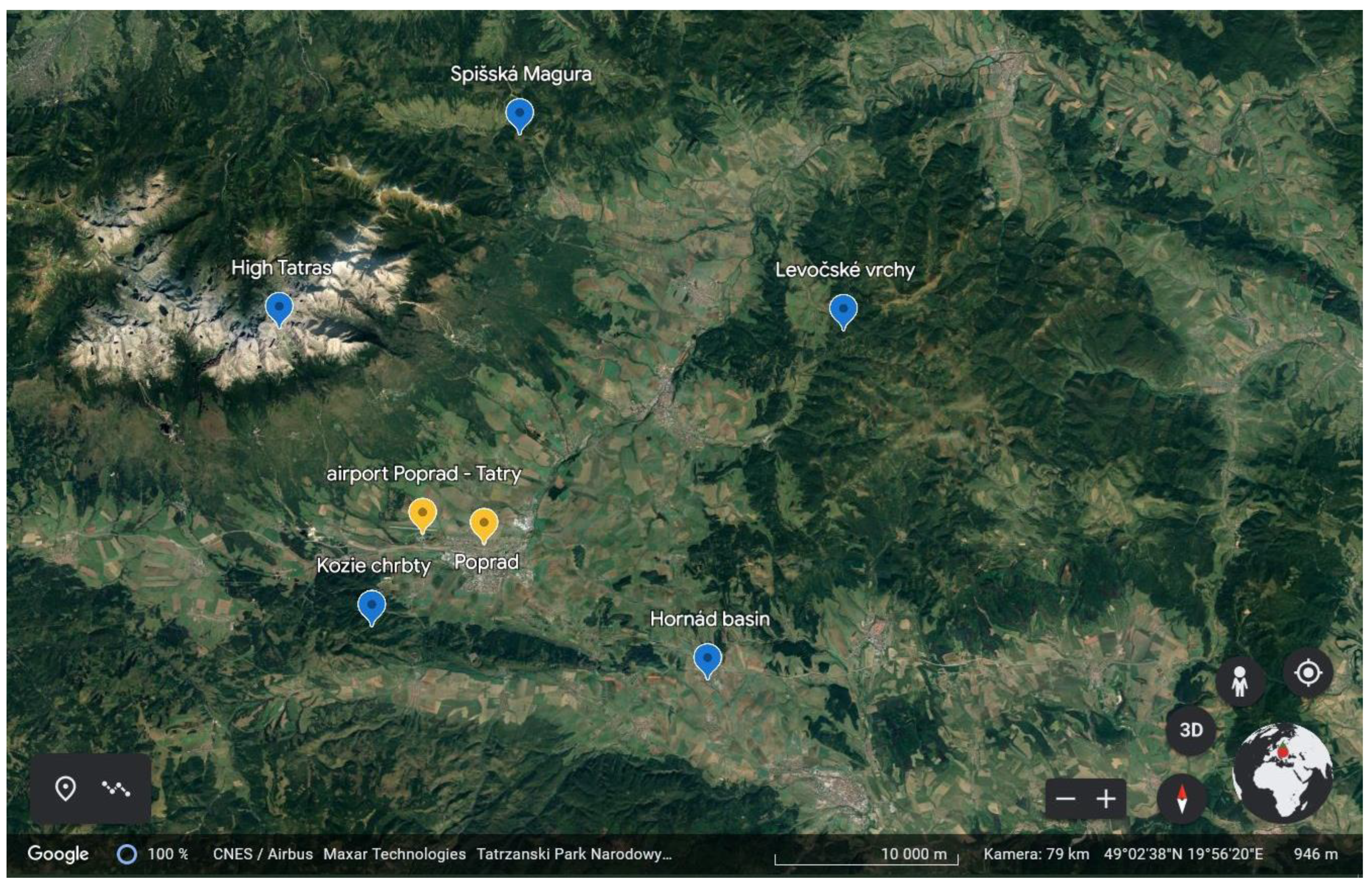
2. Description of Studied Area

The international airport Poprad-Tatry is situated on the outskirts of the town Poprad, in the region of Prešov, Northern Slovakia (Figure 1). Poprad lies in the Poprad basin that is surrounded from the north by the High Tatras and the mountain range Spišská Magura, from the east by the mountain range Levočské vrchy and from the south by the mountain range Kozie chrbty and the Hornád basin. From the west, the Poprad basin continues to the Liptov basin (Figure 2). With an altitude of 570 m above sea level (the bottom of the basin), the Poprad basin is the highest intermountain basin in Slovakia. The airport itself is situated at an altitude of 718 m above sea level, which is what makes it one of the highest-placed airports in Europe. The massive and rugged mountain terrain that encircles the basin influences the climatic conditions in the area significantly. The orientation of the basin, its openness to the west, as well as the mountain barrier of the High Tatras determine the major direction of wind blowing in this region [52].
The meteorological station Poprad (indication 11,934) lies in close proximity to the airport. The mast for wind measurements is within the measuring plot of standard dimensions—20 × 20 m. The GPS coordinates are 49.06806, 20.24972 (refers to the measuring plot); the altitude of the station is 694 m above sea level. According to the internal instruction of the Slovak Hydrometeorological Institute (SHMI), the measuring plot must be flat, without depressions, covered with grass. The weather station is surrounded by a big garden; the general surroundings are absolutely free. The height for measuring the wind direction and speed, respectively, at the monitoring station was standardised to 10 m above the ground. For measuring the wind characteristics, there are currently used Vaisala automatic instruments and GILL ultrasonic instruments. The anemometers have a 2-year calibration interval. In meteorological practice, the direction and the power of a wind vector are recorded separately as the wind direction and the wind speed. The direction of wind is determined by the direction from which the wind blows. It is measured by wind vanes at meteorological stations and recorded as the average direction of wind in the past 10 min [53].

3. Wind Speed Data Characteristics and Analysis

Usually, a 30-year period is considered necessary to estimate the long-term wind conditions at a certain location, but a period of at least 10 years may be sufficient to obtain an acceptable estimate [55]. The data used in this study were collected over a 17-year period (2005–2021) and counted a total of 148,001 wind speed measured data. Throughout the quality check, errors and missing data were removed from the analysis. After the check, the percentage of data removed was very low—0.68%; this indicates a high reliability of the monitoring system.
The data were analysed and modelled as a whole. Further, they were split into groups by months and seasons—these datasets were analysed and modelled, too. Table 1, Table 2 and Table 3 present the descriptive statistics of the monthly, seasonal, and total wind speed, including the mean, minimum, maximum, standard deviation, upper and lower quartile, median, coefficient of variation, skewness, and kurtosis.
Monthly wind speed analysis (Table 1): It was observed that during the studied period, the lowest monthly mean wind speed with value of 2.75 m/s was in August, while in March there was the highest mean wind speed with value of 3.85 m/s. The standard deviation was used to assess the variability in the wind speed. Here, the standard deviation varied from 1.86 m/s in August to 2.87 m/s in January. In general, the winter and spring months have a higher mean wind speed and variability in the wind speed than the summer and autumn months. The coefficient of variation (CV) is useful for identifying months with a higher variability in the wind speed. According to [56], the value of the CV > 40% is classified as a very high variability and CV > 70% indicates an extremely high variability in the wind speed. The coefficient of variation ranged from 66.10% in June to 86.49% in January. Based on this, the results imply that the wind speed in all months could be classified as having very high variability. During the months of September–March, there was an observed extremely high variability in the wind speed in this location. Skewness and kurtosis measure the asymmetry and the peakness of the wind speed distribution, respectively. The coefficients of skewness ranged from 0.95 in March to 1.31 in November, indicating that all distributions were right skewed. Because skewness for all months was greater than 1, the wind speed data could be regarded as highly right skewed, except for March, when the skewness of 0.95 corresponded to a moderately right skewed distribution. The coefficient of kurtosis ranged from 3.31 in March to 4.57 in August. This indicated a highly leptokurtic distribution when compared to the normal distribution.
Seasonal wind speed analysis (Table 2): The results show that the highest seasonal mean wind speed was observed in spring with value of 3.56 m/s, whereas in autumn, there was observed the lowest mean wind speed with value of 2.97 m/s. CV ranged from 67.81% to 85.27% what indicates a very high variability of wind speed in this location. The coefficient of skewness for all seasons ranged from 1.10 to 1.32. That implies that distributions are highly right skewed. The coefficient of kurtosis ranged from 3.91 to 4.44, therefore the distributions can be regarded as highly leptokurtic distributions.
Analysis of wind speed data as a whole (Table 3): The mean wind speed of 3.19 m/s was observed with a standard deviation of 2.41 m/s. The CV of 75.56%, skewness of 1.25, and kurtosis of 4.32 revealed that the wind speed data had extremely high variability in terms of the wind speed, were highly right skewed, and highly leptokurtic.

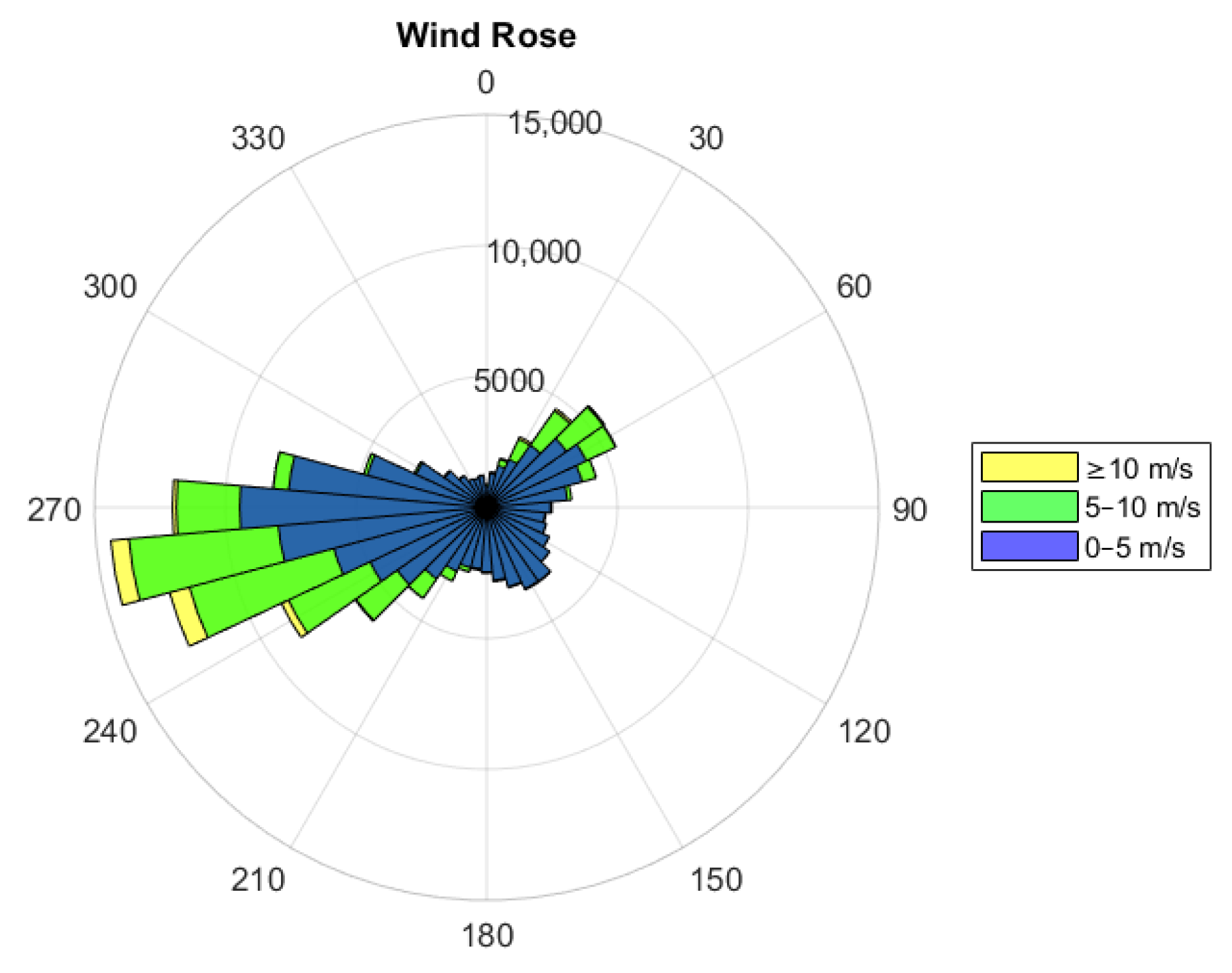
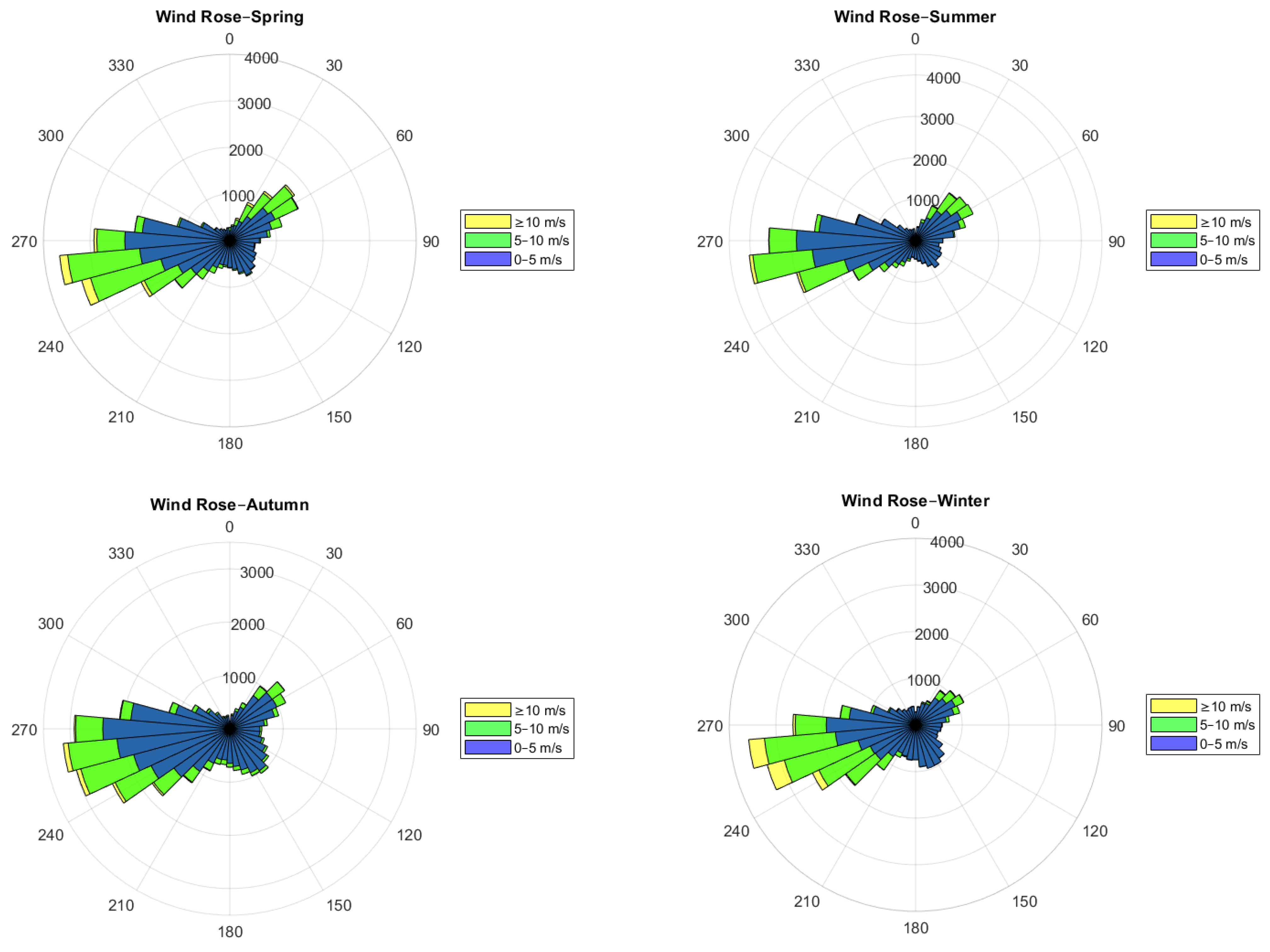
4. Wind Direction Analysis

Based on the available wind data, the wind directions were analysed. The wind rose diagrams show the temporal distribution of the wind direction at a given location. Here, the common form of the wind rose diagram was used, consisting of 36 evenly spaced sectors that were prepared using [57]. The wind rose was drawn for each season and for the whole studied period 2005–2021, as shown in Figure 3 and Figure 4.
As we may see in Figure 3, the most prevailing direction was west (W), with an occurrence rate of 34.99% and mean wind speed of 3.91 m/s during the whole study period 2005–2021. On the other hand, wind blowing from the north (N) featured the lowest occurrence rate among all directions, with only 4.45%, and a mean wind speed of 1.99 m/s. A large difference of up to 1.92 m/s can be observed between the mean wind speed blowing from the west and from the north. As it is obvious from Figure 4, the western wind direction was dominant in all seasons, with an occurrence rate ranging from 33.02% in the winter to 38.73% in the summer.

5. Methods

In this section, we provide brief information about selected probability distributions; further, the estimation method (maximum likelihood method) is characterised and the equations for the estimation of parameters of each respective distribution are given. Finally, we summarise the criteria that are applied to assess the goodness-of-fit.

5.1. Probability Distributions

A random variable X, here the wind speed, is said to have the 2-parameter Weibull distribution W(a, b) with parameters a > 0, b > 0 if its probability density function (PDF) for x ≥ 0 is given by,
f ( x ) = a b a x a 1   exp ( (   x b   ) a   )
and cumulative distribution function (CDF) is given by,
F ( x ) = 1 exp ( (   x b   ) a   )
where a is the dimensionless shape parameter and b is the scale parameter in units of the wind speed, here in m/s. The parameter a specifies the shape of the Weibull distribution, which sets the width of the wind speed data distribution. The shape factor determines the consistency of the wind speed at a particular location. It is known that, generally, a varies from 1.5 to 3 for most wind speed conditions in the world [58,59]. Small values of a signify very variable winds, while less variable winds are characterised by higher values of a. The scale parameter b determines the abscissa scale of the wind speed data distribution. It is proportional to the mean wind speed, with higher values for the locations with strong wind and lower values for still locations.
A random variable X is said to have the 3-parameter Weibull distribution W(a, b, c) with parameters a > 0, b > 0, c ≥ 0 if its PDF for xc is given by,
f ( x ) = a b a ( x c ) a 1 exp ( (   x c b   ) a   )
and its CDF is given by,
F ( x ) = 1 exp ( (   x c b   ) a   )
where a is the dimensionless shape parameter, b is the scale parameter, and c is the location parameter.
The exponentiated distribution is obtained by raising the base CDF to the positive parameter γ. A random variable X is said to have the exponentiated distribution if its CDF F(x) and PDF f(x) are given by,
F ( x ) = [ G ( x ) ] γ ,
f ( x ) = γ [ G ( x ) ] γ 1 g ( x )  
where γ > 0, and G(x) and g(x) are CDF and PDF of the base distribution, respectively. Mudholkar and Srivastava in [39] applied exponentiation to the 2-parameter Weibull distribution to obtain the exponentiated Weibull distribution. A random variable X is said to have the exponentiated Weibull distribution E W ( a ,   b , γ ) with parameters a > 0 , b > 0 ,   γ > 0 if its PDF for x > 0 is given by,
f ( x ) = γ a b ( x b ) a 1 [ 1 exp ( (   x b   ) a   ) ] γ 1 exp ( ( x b ) a )
and its CDF is given by,
F ( x ) = [ 1 exp ( (   x b   ) a   ) ] γ .
Here both a, γ are shape parameters and b is a scale parameter. For γ = 1, we obtain the 2-parameter Weibull distribution. The more detailed explanation and further information for the EW distribution can be found in [39,42,45].
In further text, we will use the following abbreviations for the probability distributions: 2-parameter Weibull—W2, 3-parameter Weibull—W3, and exponentiated Weibull—EW.

5.2. Parameter Estimation

Among various methods for estimating the parameters of the probability distribution, the maximum likelihood method (MLM) is the most preferred one due to its good asymptotic properties, including efficiency and consistency. Chang in [60] compared six methods for estimating the parameters of the Weibull distribution and showed that the MLM provided more accurate estimates than other methods in both the simulated and observed datasets. Azad et al. in [61] proposed the method of moments (MOM) and the MLM as the most efficient methods for estimating the parameters of W2 based on a comparative study of seven estimation methods. Shoaib et al. in [62] compared the MLM with the modified MLM and the Energy pattern factor method (EPF) in estimating the parameters of W2 using ten-minute averaged wind speed data from Jhampir, Pakistan. Based on the results of the root mean square error, the coefficient of determination and the χ2 test, they demonstrated better performance of the MLM as compared to the others. Many authors have used the MLM as the method for parameter estimation when modelling the wind speed using various probability distributions, for example, in [63,64]. Therefore, the MLM was utilised for estimating the parameters in this study.
The log-likelihood function ln L = ln L ( x 1 , x 2 ,   , x n ; θ ) of the probability distribution with PDF f ( x , θ ) is defined as,
ln L ( x 1 , x 2 ,   , x n ; θ ) = i = 1 n ln f ( x i ; θ )
where θ Θ is the unknown parameter (in general, it is a vector parameter), and x 1 , x 2 , , x n is a realization of the random sample X 1 ,   X 2 ,   ,   X n of size n from the distribution with PDF f ( x , θ ) . After taking the partial derivatives of the log-likelihood function ln L with respect to each parameter and equating each derivative to zero, the likelihood equations are obtained. The solution to these equations is called the maximum likelihood estimate of the parameters. The log-likelihood functions of the W2, W3, and EW distributions, respectively, and their likelihood equations are given in Table 4. As we may see, in the majority of cases the likelihood equations need to be solved iteratively.

5.3. Goodness-of-Fit and Model Selection Criteria

After estimating the parameters of the probability distribution model, it is necessary to assess the goodness-of-fit (GOF) of this model. The GOF criteria show how well the selected model fits the wind speed data, and they also indicate the applicability of the model to describe the behaviour of the data at given locations. Assessing the performance of different probability distribution models is necessary to provide more accurate information about their performance and to compare these models among themselves. Finding a more precise model helps to better understand the wind speed at a given location. In this study, we applied commonly used GOF tests—the Kolmogorov–Smirnov (KS) test and the Anderson–Darling (AD) test. Further, the information criteria, namely Akaike’s information criterion (AIC) and Bayesian information criterion (BIC), the root mean square error (RMSE), and the coefficient of determination (R2) were used. Employed GOF tests and model selection criteria are briefly described below.
The GOF tests were used to decide whether the data followed the specified theoretical distribution. The Kolmogorov–Smirnov (KS) test exploits the CDF of the probability distribution. The KS test statistic represents the largest vertical difference between the theoretical and the empirical CDF:
D = max 1 i n [ | F ^ ( x ( i ) ) i 1 n | , | i n F ^ ( x ( i ) ) | ]
where F ^ ( x ) is the estimated cumulative distribution function, x ( 1 ) ,   x ( 2 ) ,   ,   x ( n ) are observations in ascending order, i.e., x ( 1 ) x ( 2 )   x ( n ) , and F n ( x ) = 1 n   i = 1 n I ( x ( i ) x ) is the empirical distribution function, where I ( x ( i ) x ) is an indicator function assuming the value 1 if x ( i ) x and 0 otherwise. The null hypothesis that the data follow the distribution under test, is rejected at the chosen significance level α if the test statistic D > D ( α ) , where D ( α ) is a critical value of the KS test. The smaller the value of the test statistic D , the better the fit.
The Anderson–Darling (AD) test is a modification of the KS test. This test is considered to be a better GOF test because it gives more weight to the tails of the distribution than the KS test does. According to studies [65,66], the AD test was ranked as one of the most powerful tests for detecting deviations from the Weibull and the extreme value distributions. The AD test statistic is defined as follows:
A 2 = n i = 1 n 2 i 1 n [ ln ( F ^ ( x ( i ) ) ) + ln ( 1 F ^ ( x ( n + 1 i ) ) ) ] .
The null hypothesis that data follow the specified distribution, is rejected at the significance level α if the test statistic A2 is greater than the critical value of the AD test. Again, the smaller value of the test statistic A2 indicates a better fit.
The application of the maximum likelihood method (MLM) for the parameter estimation allows us to use the information criteria—Akaike’s information criterion (AIC) and Bayesian information criterion (BIC)—to decide the GOF for the distributions. The AIC and the BIC are defined as follows [67,68]
A I C = 2 ln L + 2 k ,
B I C = 2 ln L + k ln n
where ln L is the maximum value of the log-likelihood function for the estimated model, k is number of estimated parameters, and n is the sample size. Furthermore, the coefficient of determination (R2) and the root mean square error (RMSE) are considered to decide on the best fitting model. The RMSE determines the accuracy of the model by calculating the average of the square difference between the observed and the predicted probabilities of the theoretical distribution. The R2 is used to measure the linear relationship between the observed and the predicted probabilities of the theoretical distribution. The RMSE and R2 are calculated by:
R M S E = ( 1 n i = 1 n [ F n ( x i ) F ^ ( x i ) ] 2 ) 1 2 ,
R 2 = i = 1 n [ F ^ ( x i ) F ¯ ] 2 i = 1   n [ F ^ ( x i ) F ¯ ] 2 + i = 1 n [ F n ( x i ) F ^ ( x i ) ] 2  
where F ¯ = 1 n   i = 1 n F ^ ( x i ) .
In general, lower values of KS, AD, AIC, BIC, RMSE, and a higher value of R2 indicate better fit of the theoretical distribution to the wind speed data as compared to the others.

6. Results and Discussion
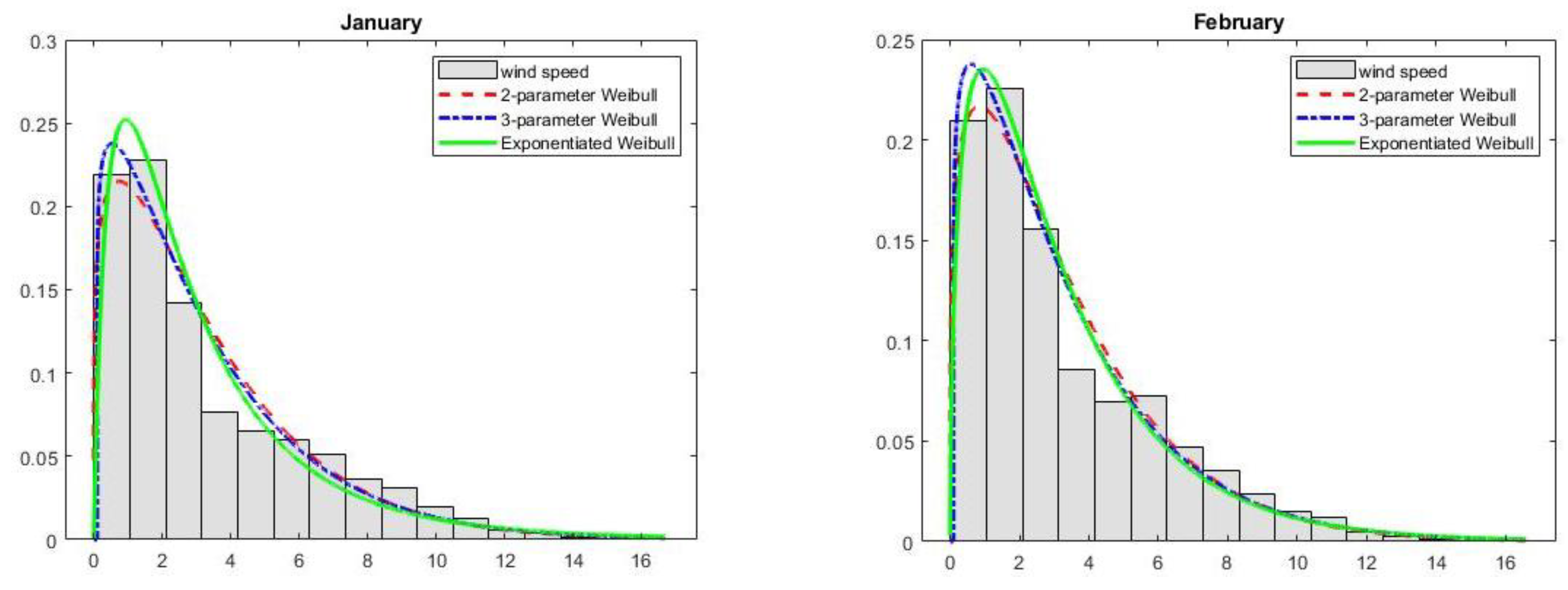
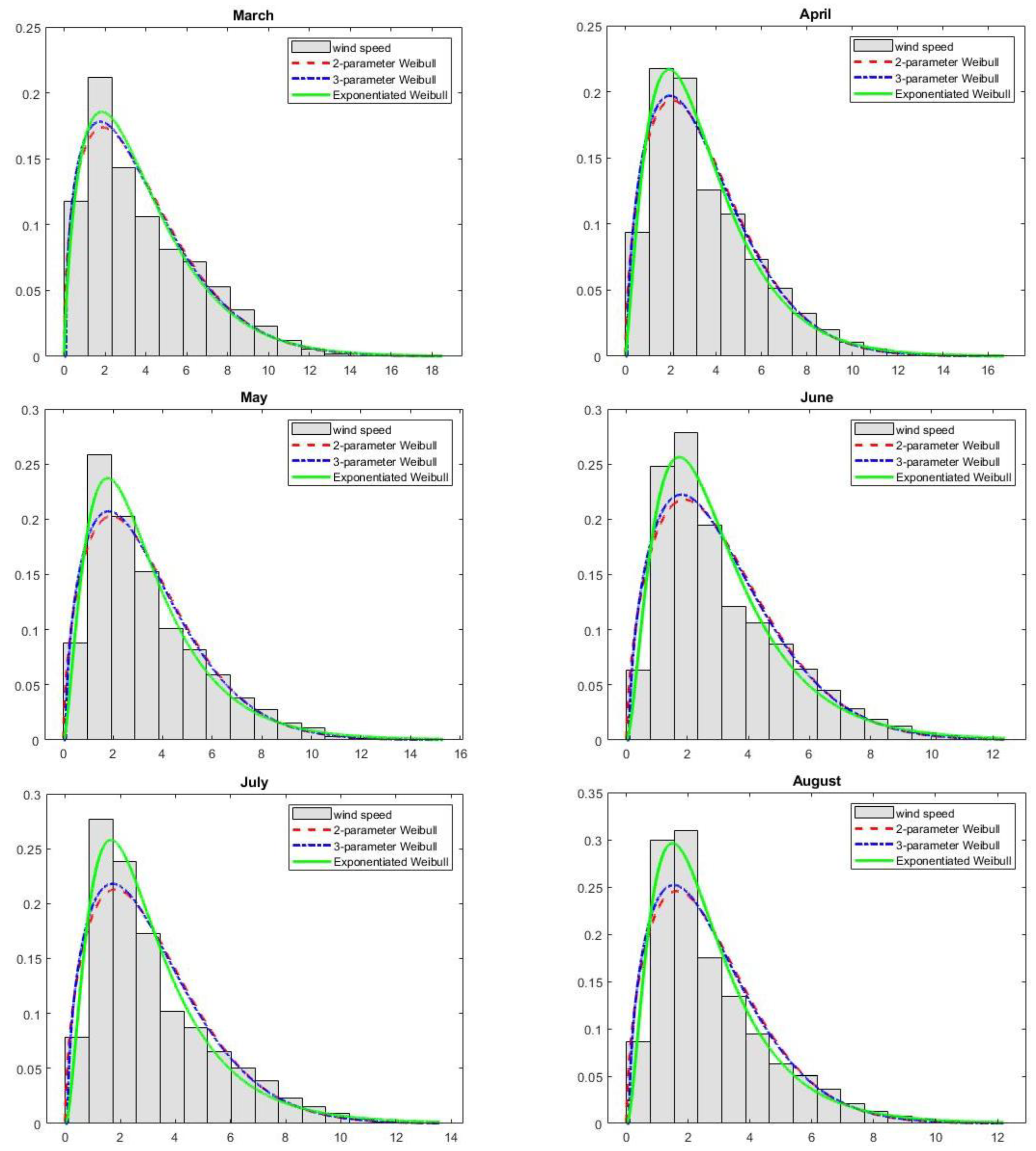
Three probability distributions, namely 2-parameter Weibull, 3-parameter Weibull, and exponentiated Weibull, were applied to fit the wind speed data from the meteorological station Poprad, located at the Poprad-Tatry airport. Their performance was compared in terms of how well these distributions matched the observed wind speed data. Applying the maximum likelihood method, we obtained the parameter estimates for all discussed probability distributions. The evaluation of each model was done by the GOF tests and the model selection criteria described in Section 5.3. The estimated parameters as well as test statistics of the KS and the AD tests, respectively, and of the other assessing criteria are summarised below in Table 5, Table 6, Table 7 and Table 8—for the estimated parameters of the probability distributions see Table 5 (the entire period and the seasons) and Table 7 (respective months); for the GOF tests and model selection criteria see Table 6 (the entire period and the seasons), and Table 8 (respective months).
Figure 5, Figure 6 and Figure 7 illustrate how appropriately the considered probability distributions describe the wind speed data.
From the obtained results and their visualizations, we can conclude the following:
  • Respective months:
For eight out of the twelve months (April–November), the EW distribution achieved the best results in terms of all GOF tests and the model selection criteria. In February and March, W3 performed better, but the EW was the second best. In January and December, the EW and the W3 distribution ranked the same, but the EW performed better in terms of the KS and the AD test, as well as in terms of R2, and RMSE. In this case, when some GOF tests and model selection criteria favoured the EW distribution, whereas the others the W3 distribution, we made a conclusion according to the value of the AD test since the AD test is considered as a more powerful GOF test. Furthermore, according to conclusions drawn in [69], R2 appears to be more informative than the other indicators in such cases. Therefore, when choosing the most suitable distribution for a given month, the probability distribution with the smallest value of the AD test and the highest R2 value was selected as the best fitting distribution for the wind speed data in that month. According to this, the EW distribution was more suitable for January and December. Such assumptions agree with the visualization in Figure 7, where the theoretical distributions fitted to the observed data in the months January and December show that the EW distribution was closer to the empirical distribution than the W3 distribution.
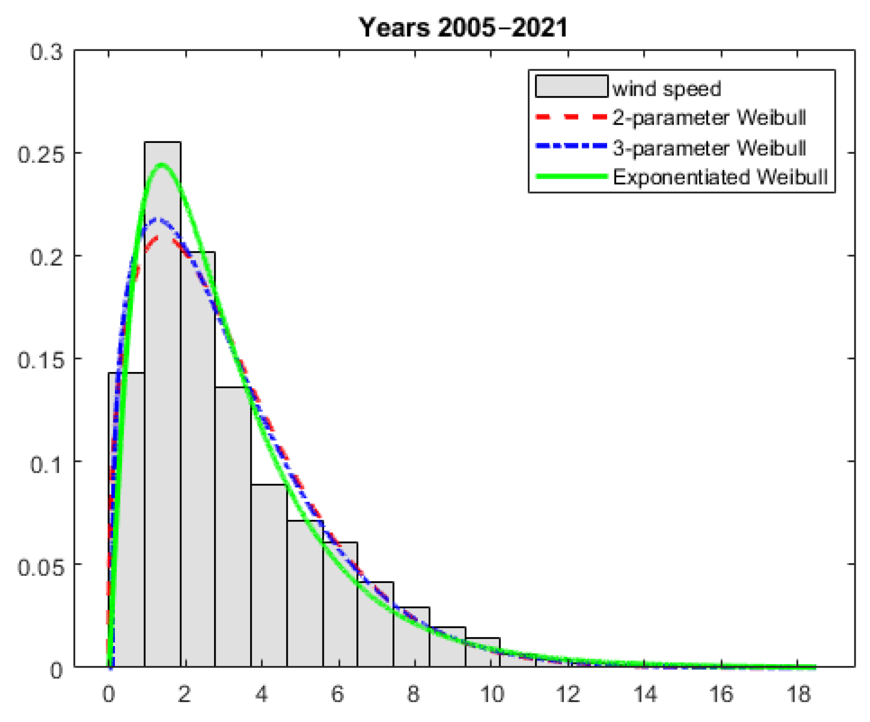
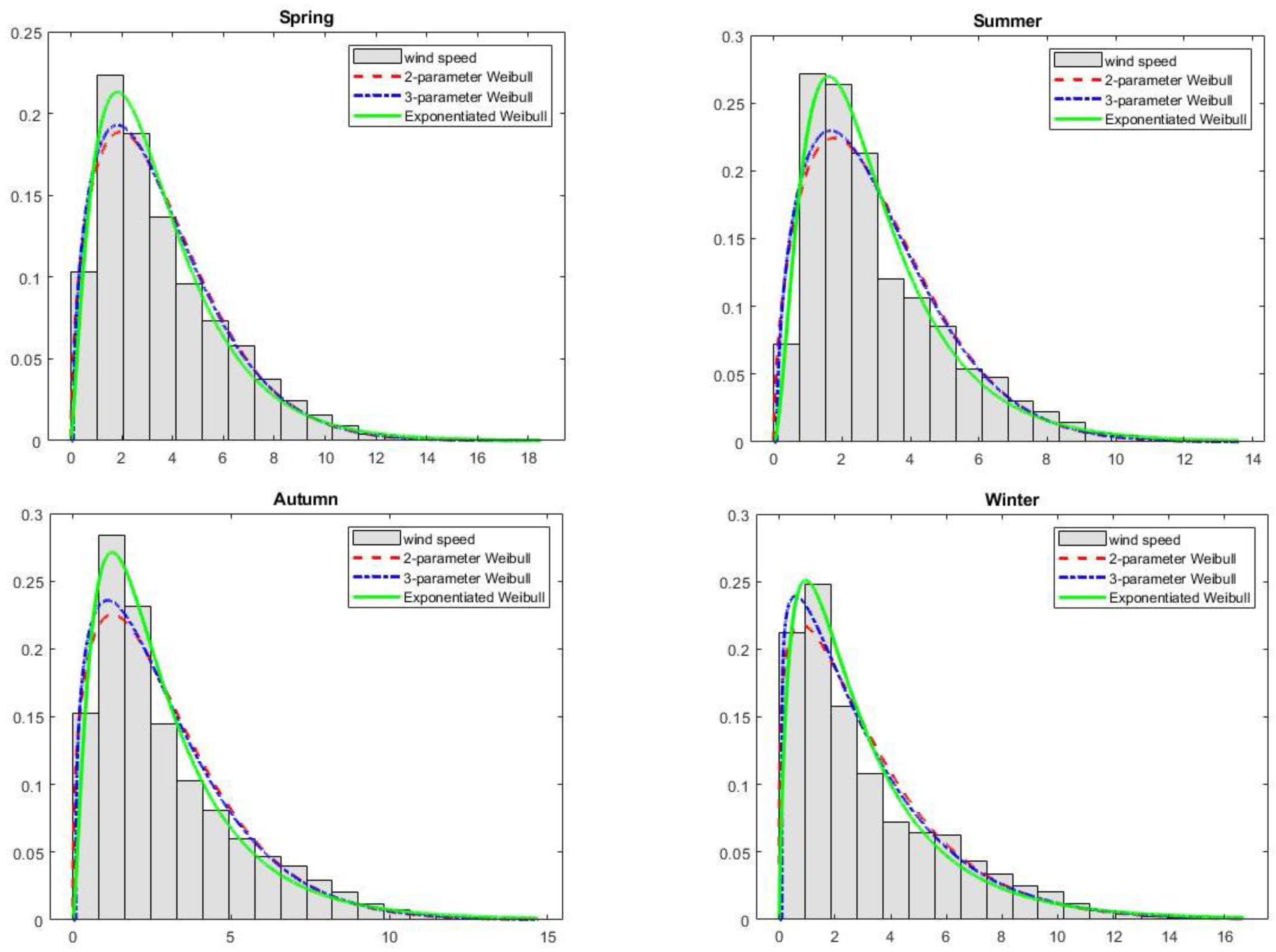
  • The entire period and the seasons:
After the visual inspection of Figure 5 and Figure 6, we see that the EW distribution was closer to the empirical distribution than the other two distributions. This observation was supported by the results of the GOF tests and of the model selection criteria (Table 6), where the EW distribution obtained the highest value of R2 and the lowest values of all the other criteria, except for the winter. In the winter, the W3 distribution obtained better results for the information criteria. However, the EW distribution had the highest value of the coefficient of determination and the lowest values of the AD test and the RMSE among the discussed distributions. This indicated that the EW distribution demonstrated a better fit than the other two distributions. Thus, the EW distribution was more suitable for modelling the wind speed in this location for the entire studied period and for all the seasons. According to the criteria, W3 performed as the second best.
We may conclude that for the considered datasets the EW distribution exhibited a significantly better fit to the wind speed data than the W2 and W3 distributions. It is obvious, that the EW distribution had superiority over the W2 and W3 distribution in modelling the peakness of the data. Further, because the EW distribution had larger right tail probability than the W2 and W3 distributions, this provided more flexibility for the EW distribution to model datasets where extreme strong winds or outliers in the direction of the right tail occurred.
When we compare our findings with those in [49,50], we can notice several similarities:
  • The datasets in both other papers had high values of kurtosis—in the dataset from [49], the kurtosis was 2.502; in the datasets from [50], the values of kurtosis ranged from 3.877 to 8.806. The datasets here, with the EW distribution as the most suitable one, also possessed high values of the coefficient of kurtosis, ranging from 3.31 to 4.57.
  • The datasets in both other papers had positive values of skewness—in the dataset from [49], the skewness was 0.633; in the datasets from [50], the values of skewness ranged from 0.888 to 2.014. The datasets, modelled here, also had values of the coefficient of skewness ranging from 0.95 to 1.31. All of these datasets can be regarded as moderate to highly right skewed.
Thus, the EW distribution can be used as a theoretical probability distribution for modelling the datasets of the wind speed with high positive skewness and kurtosis.

7. Conclusions

The determination of an appropriate wind speed distribution for modelling wind speed data is important for determining the wind profile in a specific location. In this work, we proposed the use of the exponentiated Weibull distribution to describe the wind speed data obtained from the location Poprad airport. The position of the airport at the altitude of 718 m above sea level at the foothills creates specific conditions that influence the operation and safety of the flights. In the article, we examined the wind speed in this location. Based on long-term observations, it is possible to predict how the wind speed will develop in a given location. Here, we showed that the EW distribution is more appropriate for modelling the wind speed data than the W2 and W3 distributions, which are commonly used in the literature. This result is based on the values of six GOF indicators—the KS test, the AD test, AIC, BIC, RMSE, and R2. The EW distribution performed the best (in comparison to values of the indicators for the W2 and W3 distributions, respectively) and provided a better fit to the seasonal and monthly wind speed data, except for February and March, when the W3 performed better, but the EW was the second best. Therefore, the EW distribution can be considered as a suitable wind speed distribution and can be applied to forecast and estimate the wind speed at the meteorological station Poprad. Based on the character of the studied data in terms of their skewness, we can also recommend the EW distribution as a good model for highly right skewed data. In addition, the EW distribution is flexible enough in terms of modelling the peakness of the data. To sum it up, the EW distribution proved to be a good alternative to the W2 and W3 distributions due to its flexibility in modelling the data of the wind speed with high positive skewness and kurtosis.

Author Contributions

Conceptualization, I.P. and M.M.; methodology, I.P. and M.M.; software, Z.S. and M.M.; validation, I.P., M.M. and D.J.; investigation, I.P., M.M. and Z.S.; resources, D.J.; data curation, I.P. and Z.S.; writing—original draft preparation, I.P.; writing—review and editing, M.M.; visualization, Z.S. and M.M.; supervision, I.P.; project administration, I.P.; funding acquisition, I.P. All authors have read and agreed to the published version of the manuscript.

Funding

This research was funded by the Cultural and Educational Grant Agency of the Ministry of Education, Science, Research, and Sport of the Slovak Republic KEGA, grant number 029ŽU-4/2022.

Institutional Review Board Statement

Not applicable.

Informed Consent Statement

Not applicable.

Data Availability Statement

The meteorological data used in the article will be fully available by request, in order to contribute to transparency. They are not accessible publicly (only for research and publications).

Acknowledgments

The authors gratefully acknowledge the Slovak Hydrometeorological Institute for providing us with measured wind speed data, namely Peter Kajaba.

Conflicts of Interest

The authors declare no conflict of interest. The funders had no role in the design of the study; in the collection, analyses, or interpretation of data; in the writing of the manuscript; or in the decision to publish the results.

References

  1. Safari, B.; Gasore, J. A statistical investigation of wind characteristics and wind energy potential based on the Weibull and Rayleigh models in Rwanda. Renew. Energy 2010, 35, 2874–2880. [Google Scholar] [CrossRef]
  2. Chen, H.; Birkelund, Y.; Anfinsen, S.N.; Staupe-Delgado, R.; Yuan, F. Assessing probabilistic modelling for wind speed from numerical weather prediction and observation in the Artic. Sci. Rep. 2021, 11, 7613. [Google Scholar] [CrossRef] [PubMed]
  3. Lun, I.Y.F.; Lam, J.C. A study of Weibull parameters using long-term wind observations. Renew. Energy 2000, 20, 145–153. [Google Scholar] [CrossRef]
  4. Davenport, A.G. The relationship of wind structure to wind loading. In Proceedings of the Symposium No. 16—Wind Effects on Buildings and Structures, Teddington, UK, 26–28 June 1963; pp. 53–111. [Google Scholar]
  5. Hemanth Kumar, M.B.; Saravanan, B.; Sanjeevikumar, P.; Holm-Nielsen, J.B. Wind Energy Potential Assessment by Weibull Parameter Estimation Using Multiverse Optimization Method: A Case Study of Tirumala Region in India. Energies 2019, 12, 2158. [Google Scholar] [CrossRef] [Green Version]
  6. Abbas, G.; Gu, J.; Asad, M.U.; Balas, V.E.; Farooq, U.; Khan, I.A. Estimation of Weibull Distribution Parameters by Analytical Methods for the Wind Speed of Jhimpir, Pakistan—A Comparative Assessment. In Proceedings of the 2022 International Conference on Emerging Trends in Electrical, Control, and Telecommunication Engineering (ETECTE), Lahore, Pakistan, 2–4 December 2022. [Google Scholar]
  7. Hussain, I.; Haider, A.; Ullah, Z.; Russo, M.; Casolino, G.M.; Azeem, B. Comparative Analysis of Eight Numerical Methods Using Weibull Distribution to Estimate Wind Power Density for Coastal Areas in Pakistan. Energies 2023, 16, 1515. [Google Scholar] [CrossRef]
  8. Kang, S.; Khanjari, A.; You, S.; Lee, J.-H. Comparison of different statistical methods used to estimate Weibull parameters for wind speed contribution in nearby an offshore site, Republic of Korea. Energy Rep. 2021, 7, 7358–7373. [Google Scholar] [CrossRef]
  9. Salami, A.A.; Ouedraogo, S.; Kodjo, K.M.; Ajavon, A.S.A. Influence of the random data ampling in estimation of wind speed resource: Case study. Int. J. Renew. Energy Dev. 2022, 11, 133–143. [Google Scholar] [CrossRef]
  10. Dhakal, R.; Sedai, A.; Pol, S.; Parameswaran, S.; Nejat, A.; Moussa, H. A Novel Hybrid Method for Short-Term Wind Speed Prediction Based on Wind Probability Distribution Function and Machine Learning Models. Appl. Sci. 2022, 12, 9038. [Google Scholar] [CrossRef]
  11. Singh, K.A.; Khan, M.G.M.; Ahmed, M.R. Wind Energy Resource Assessment for Cook Islands with Accurate Estimation of Weibull Parameters Using Frequentist and Bayesian Methods. IEEE Access 2022, 10, 25935–25953. [Google Scholar] [CrossRef]
  12. Alsamamra, H.R.; Salah, S.; Shoqeir, J.A.H.; Manasra, A.J. A comparative study of five numerical methods for the estimation of Weibull parameters for wind energy evaluation at Eastern Jerusalem, Palestine. Energy Rep. 2022, 8, 4801–4810. [Google Scholar] [CrossRef]
  13. Al-Hussieni, A.J.M. A prognosis of wind energy potential as a power generation source in Basra city, Iraq state. Eur. Sci. J. 2014, 10, 163–176. [Google Scholar]
  14. Okakwu, I.; Akinyele, D.; Olabode, O.; Ajewole, T.; Oluwasogo, E.; Oyedeji, A. Comparative Assessment of Numerical Techniques for Weibull Parameters’ Estimation and the Performance of Wind Energy Conversion Systems in Nigeria. IIUM Eng. J. 2023, 24, 138–157. [Google Scholar] [CrossRef]
  15. Shu, Z.R.; Jesson, M. Estimation of Weibull parameters for wind energy analysis across the UK. J. Renew. Sustain. Energy 2021, 13, 023303. [Google Scholar] [CrossRef]
  16. Truhetz, H.; Krenn, A.; Winkelmeier, H.; Müller, S.; Cattin, R.; Eder, T.; Biberacher, M. Austrian Wind Potential Analysis (AuWiPot). In Proceedings of the 12. Symposium Energieinnovation, Graz, Austria, 15–17 February 2012. [Google Scholar]
  17. Pobočíková, I.; Sedliačková, Z.; Šimon, J.; Jurášová, D. Statistical analysis of the wind speed at mountain site Chopok, Slovakia, using Weibull distribution. IOP Conf. Ser. Mater. Sci. End. 2020, 776, 012114. [Google Scholar] [CrossRef]
  18. Wais, P. A review of Weibull functions in wind sector. Renew. Sust. Energ. Rev. 2017, 70, 1099–1107. [Google Scholar] [CrossRef]
  19. Carta, J.A.; Ramírez, P.; Velázquez, S. A review of wind speed probability distributions used in wind energy analysis: Case studies in the Canary Islands. Renew. Sust. Energ. Rev. 2009, 13, 933–955. [Google Scholar] [CrossRef]
  20. Akgül, F.G.; Şenoğlu, B.; Arslan, T. An alternative distribution to Weibull for modeling the wind speed data: Inverse Weibull distribution. Energy Convers. Manag. 2016, 114, 234–240. [Google Scholar] [CrossRef]
  21. Sukkiramathi, K.; Seshaiah, C. Analysis of wind power potential by the three-parameter Weibull distribution to install a wind turbine. Energy Explor. Exploit. 2020, 38, 158–174. [Google Scholar] [CrossRef] [Green Version]
  22. Pobočíková, I.; Sedliačková, Z.; Michalková, M. Application of four probability distributions for wind speed modeling. Procedia Eng. 2017, 192, 713–718. [Google Scholar] [CrossRef]
  23. Sarkar, A.; Singh, S.; Mitra, D. Wind climate modeling using Weibull and extreme value distribution. Int. J. Eng. Sci. Technol. 2011, 3, 100–106. [Google Scholar] [CrossRef]
  24. Morgan, E.C.; Lackner, M.; Vogel, R.M.; Baise, L.G. Probability distributions for offshore wind speeds. Energy Convers. Manag. 2011, 52, 15–26. [Google Scholar] [CrossRef]
  25. Kang, D.; Ko, K.; Huh, J. Determination of extreme wind values using the Gumbel distribution. Energy 2015, 86, 51–58. [Google Scholar] [CrossRef]
  26. Alavi, O.; Mohammadi, K.; Mostafaeipour, A. Evaluating the suitability of wind speed probability distribution models: A case study of east and southeast parts of Iran. Energy Convers. Manag. 2016, 119, 101–108. [Google Scholar] [CrossRef]
  27. Mohammadi, K.; Alavi, O.; McGowan, J.G. Use of Birnbaum-Saunders distribution for estimating wind speed and wind power probability distributions: A review. Energy Convers. Manag. 2017, 143, 109–122. [Google Scholar] [CrossRef]
  28. Jung, C.; Schindler, D. Global comparison of the goodness-of-fit of wind speed distributions. Energy Convers. Manag. 2017, 133, 216–234. [Google Scholar] [CrossRef]
  29. Kantar, Y.M.; Usta, I.; Arik, I.; Yenilmez, I. Wind speed analysis using the Extended Generalized Lindley Distribution. Renew. Energy 2018, 118, 1024–1030. [Google Scholar] [CrossRef]
  30. Ahmad, Z.; Mahmoudi, E.; Roozegarz, R.; Hamedani, G.G.; Butt, N.S. Contributions towards new families of distributions: An investigation, further developments, characterizations and comparative study. Pak. J. Stat. Oper. Res. 2022, 18, 99–120. [Google Scholar] [CrossRef]
  31. Marshall, A.W.; Olkin, I. A new method for adding a parameter to a family of distributions with application to the exponential and Weibull families. Biometrika 1997, 84, 641–652. [Google Scholar] [CrossRef]
  32. ul Haq, M.A.; Rao, G.S.; Albassam, M.; Aslam, M. Marshall-Olkin Power Lomax distribution for modeling of wind speed data. Energy Rep. 2020, 6, 1118–1123. [Google Scholar] [CrossRef]
  33. Carta, J.A.; Ramírez, P. Analysis of two-component mixture Weibull statistics for estimation of wind speed distributions. Renew. Energy 2007, 32, 518–531. [Google Scholar] [CrossRef]
  34. Akpinar, S.; Akpinar, E.K. Estimation of wind energy potential using finite mixture distribution models. Energy Convers. Manag. 2009, 50, 877–884. [Google Scholar] [CrossRef]
  35. Kollu, R.; Rayapudi, S.R.; Narasimham, S.V.L.; Pakkurthi, K.M. Mixture probability distribution functions to model wind speed distributions. Int. J. Energy Environ. Eng. 2012, 3, 27. [Google Scholar] [CrossRef] [Green Version]
  36. Ouarda, T.B.M.J.; Charron, C. On the mixture of wind speed distribution in a Nordic region. Energy Convers. Manag. 2018, 174, 33–44. [Google Scholar] [CrossRef]
  37. Mahbudi, S.; Jamalizadeh, A.; Farnoosh, R. Use of finite mixture models skew-t-normal Birnbaum-Saunders components in the analysis of wind speed: Case studies in Ontario, Canada. Renew. Energy 2020, 162, 196–211. [Google Scholar] [CrossRef]
  38. Gupta, R.C.; Gupta, P.L.; Gupta, R.D. Modeling failure time data by Lehman alternatives. Commun. Stat.-Theory Methods 1998, 27, 887–904. [Google Scholar] [CrossRef]
  39. Mudholkar, G.S.; Srivastava, D.K. Exponentiated Weibull family for analysing bathtub failure-rate data. IEEE Trans. Reliab. 1993, 42, 299–302. [Google Scholar] [CrossRef]
  40. Mudholkar, G.S.; Srivastava, D.K.; Freimer, M. The exponentiated Weibull family: A reanalysis of the bus-motor-failure data. Technometrics 1995, 37, 436–445. [Google Scholar] [CrossRef]
  41. Mudholkar, G.S.; Hutson, A.D. The exponentiated Weibull family: Some properties and a flood data application. Commun. Stat.-Theory Methods 1996, 25, 3059–3083. [Google Scholar] [CrossRef]
  42. Nassar, M.M.; Eissa, F.H. On the exponentiated Weibull distribution. Commun. Stat.-Theory Methods 2003, 32, 1317–1336. [Google Scholar] [CrossRef]
  43. Nassar, M.M.; Eissa, F.H. Bayesian estimation for the exponentiated Weibull model. Commun. Stat.-Theory Methods 2004, 33, 2343–2362. [Google Scholar] [CrossRef]
  44. Alizadeh, M.; Bagheri, S.F.; Baloui Jamkhaneh, E.; Nadarajah, S. Estimates of the PDF and the CDF of the exponentiated Weibull distribution. Braz. J. Probab. Stat. 2015, 29, 695–716. [Google Scholar] [CrossRef]
  45. Nadarajah, S.; Kotz, S. On the moments of the exponentiated Weibull distribution. Commun. Stat.-Theory Methods 2005, 34, 253–256. [Google Scholar] [CrossRef]
  46. Salem, A.M.; Abo-Kasem, O.E. Estimation for the parameters of the exponentiated Weibull distribution based on progressive hybrid censored samples. Int. J. Contemp. Math. Sci. 2011, 6, 1713–1724. [Google Scholar]
  47. Pal, M.; Ali, M.M.; Woo, J. Exponentiated Weibull distribution. Statistica 2006, 66, 136–147. [Google Scholar] [CrossRef]
  48. Barrios, R.; Dios, F. Exponentiated Weibull distribution family under aperture averaging for Gaussian beam waves. Opt. Express 2012, 20, 13055–13064. [Google Scholar] [CrossRef] [Green Version]
  49. Shittu, O.I.; Adepoju, K.A. On the exponentiated Weibull distribution for modeling wind speed in South Western Nigeria. J. Mod. Appl. Stat. Methods 2014, 13, 431–445. [Google Scholar] [CrossRef] [Green Version]
  50. Akgül, F.G.; Şenoğlu, B. Comparison of wind speed distributions: A case study for Aegean coast of Turkey. Energy Sources A Recovery Util. Environ. Eff. 2019, 45, 2453–2470. [Google Scholar] [CrossRef]
  51. Unesco. Tatra Transboundary Biosphere Reserve, Poland/Slovakia. Available online: https://www.unesco.org/en/man-and-biosphere/tatra-transboundary-biosphere-reserve-poland/slovakia-0 (accessed on 11 March 2023).
  52. Ilčin, J. Problematics of Flight in Mountainous Terrain. Bachelor’s Thesis, Brno University of Technology, Brno, Czech Republic, 2017. [Google Scholar]
  53. Bochníček, O.; Hrušková, K.; Zvara, I. Climate Atlas of Slovakia, 1st ed.; Slovak Hydrometeorological Institute: Bratislava, Slovakia, 2015; p. 131. [Google Scholar]
  54. Google Earth. Available online: https://earth.google.com/web/search/Poprad,+Slovakia/@49.05877989,20.29744794,672.117089a,24378.01462403d,35y,0h,0t,0r/data=CnsaURJLCiUweDQ3M2UzYTk0YmNmZGExOTE6MHg5Mzk3NGEwYWVmODZiOTIwGSrNQSuLhkhAIdHHfECgSzRAKhBQb3ByYWQsIFNsb3Zha2lhGAIgASImCiQJI8yHUE9QNUARIcyHUE9QNcAZKLUxbvu7QkAhhILfAjV3UMA (accessed on 8 March 2023).
  55. Manwell, J.F.; McGowan, J.G.; Rogers, A.L. Wind Energy Explained: Theory, Design and Application, 2nd ed.; Wiley: Chichester, UK, 2010; p. 704. [Google Scholar]
  56. Hare, W. Assessment of Knowledge on Impacts of Climate Change—Contribution to the Specification of Art. 2 of the UNFCCC: Impacts on Ecosystems, Food Production, Water and Socio-Economic Systems; External Expertise Report for German Advisory Council on Global Change: Berlin, Germany, 2003; p. 104. [Google Scholar]
  57. Al Mac. Wind_Rose (Wind_Direction, Wind_Speed). MATLAB Central File Exchange. Available online: https://www.mathworks.com/matlabcentral/fileexchange/65174-wind_rose-wind_direction-wind_speed (accessed on 13 February 2023).
  58. Akpinar, E.K.; Akpinar, S. Determination of the wind energy potential for Maden-Elazig, Turkey. Energy Convers. Manag. 2004, 45, 2901–2914. [Google Scholar] [CrossRef]
  59. Akdag, S.A.; Dinler, A. A new method to estimate Weibull parameters for wind energy applications. Energy Convers. Manag. 2009, 50, 1761–1766. [Google Scholar] [CrossRef]
  60. Chang, T.P. Performance comparison of six numerical methods in estimating Weibull parameters for wind energy application. Appl. Energy 2011, 88, 272–282. [Google Scholar] [CrossRef]
  61. Azad, A.K.; Rasul, M.G.; Yusaf, T. Statistical Diagnosis of the Best Weibull Methods for Wind Power Assessment for Agricultural Applications. Energies 2014, 7, 3056–3085. [Google Scholar] [CrossRef] [Green Version]
  62. Shoaib, M.; Siddiqui, I.; Rehman, S.; Khan, S.; Alhems, L.M. Assessment of wind energy potential using wind energy conversion system. J. Clean. Prod. 2019, 216, 346–360. [Google Scholar] [CrossRef]
  63. Al-Mhairat, B.; Al-Quraaan, A. Assessment of Wind Energy Resources in Jordan Using Different Optimization Techniques. Processes 2022, 10, 105. [Google Scholar] [CrossRef]
  64. Chang, T.P. Estimation of wind energy potential using different probability density functions. Appl. Energy 2011, 88, 1848–1856. [Google Scholar] [CrossRef]
  65. Evans, J.W.; Johnson, R.A.; Green, D.W. Two- and Three-Parameter Weibull Goodness-of-Fit Tests; Res. Pap. FPL-RP-493; U.S. Department of Agricultural, Forest Service, Forest Products Laboratory: Madison, WI, USA, 1989; p. 27.
  66. Krit, M.; Gaudoin, O.; Remy, E. Goodness-of-fit tests for the Weibull and extreme value distributions: A review and comparative study. Commun. Stat.-Simul. Comput. 2021, 50, 1888–1911. [Google Scholar] [CrossRef]
  67. Akaike, H. A new look at the statistical model identification. IEEE Trans. Automat. Contr. 1974, 19, 716–723. [Google Scholar] [CrossRef]
  68. Schwarz, G. Estimating the Dimension of a Model. Ann. Stat. 1978, 6, 461–464. [Google Scholar] [CrossRef]
  69. Chicco, D.; Warrens, M.J.; Jurman, G. The coefficient of determination R-squared is more informative than SMAPE, MAE, MAPE, MSE and RMSE in regression analysis evaluation. PeerJ Comput. Sci. 2021, 7, e623. [Google Scholar] [CrossRef]
Figure 1. The location of the meteorological station in Slovakia (upper); in Poprad (lower). Source: [53,54].
Applsci 13 04031 g001
Figure 2. The topography of the Poprad basin and its surroundings. Source [54].
Applsci 13 04031 g002
Figure 3. Wind rose diagram for the whole studied period 2005–2021.
Applsci 13 04031 g003
Figure 4. Wind rose diagrams for the seasons.
Applsci 13 04031 g004
Figure 5. Modelled probability distributions fitted to the histogram of the wind speed data–the entire considered period.
Applsci 13 04031 g005
Figure 6. Modelled probability distributions fitted to the histogram of the wind speed data—the seasons.
Applsci 13 04031 g006
Figure 7. Modelled probability distributions fitted to the histogram of the wind speed data—the respective months.
Applsci 13 04031 g007aApplsci 13 04031 g007bApplsci 13 04031 g007c
Table 1. Descriptive statistics of respective months.
PeriodMeanStandard DeviationMinMaxLower QuartileMedianUpper QuartileCoefficient of Variation (%)SkewnessKurtosis
January3.312.870.116.71.12.25.086.491.213.78
February3.232.700.116.61.22.34.783.691.234.13
March3.852.730.118.51.73.15.571.040.953.31
April3.492.330.116.71.72.94.866.751.124.15
May3.332.260.115.31.62.74.567.771.174.21
June3.122.060.112.41.62.54.366.101.144.05
July3.162.170.113.61.62.54.368.461.183.99
August2.751.860.112.21.42.23.767.621.284.57
September2.922.110.114.11.42.33.972.411.294.47
October2.962.250.114.71.32.24.175.971.28 4.38
November3.032.520.114.31.12.14.283.151.314.23
December3.152.690.114.91.12.24.682.271.284.17
Table 2. Descriptive statistics of seasons.
PeriodMeanStandard DeviationMinMaxLower QuartileMedianUpper QuartileCoefficient of Variation (%)SkewnessKurtosis
Spring3.562.460.118.51.72.94.969.141.103.91
Summer3.012.040.113.61.52.44.167.811.214.24
Autumn2.972.300.114.71.32.24.177.441.324.44
Winter3.232.760.116.71.12.24.885.271.244.02
Table 3. Descriptive statistics of the whole dataset.
PeriodMeanStandard DeviationMinMaxLower QuartileMedianUpper QuartileCoefficient of Variation (%)SkewnessKurtosis
Total3.192.410.118.51.42.44.575.561.254.32
Table 4. Log-likelihood functions and likelihood equations of selected probability distributions.
DistributionMLM Estimate
W2Log-likelihood function ln L = n ln a b a 1 b a i = 1 n x i a + ( a 1 ) i = 1 n ln x i
Likelihood equations 1 a i = 1 n x i a ln x i   i = 1 n x i a + 1 n i = 1 n ln x i = 0
b = [ 1 n i = 1 n x i a ] 1 / a
W3Log-likelihood function ln L = n ln a b a 1 b a i = 1 n ( x i c ) a + ( a 1 ) i = 1 n ln ( x i c )
Likelihood equations 1 a i = 1 n ( x i c ) a ln ( x i c )   i = 1 n ( x i c ) a + 1 n i = 1 n ln ( x i c ) = 0
b = [ 1 n i = 1 n ( x i c ) a ] 1 / a
a 1 a 1 n i = 1 n ( x i c ) a i = 1 n ( x i c ) a 1 i = 1 n 1 x i c = 0
EWLog-likelihood function ln L = n ln ( γ a b a ) 1 b a i = 1 n x i a + ( a 1 ) i = 1 n ln x i + ( γ 1 ) i = 1 n ln [ 1 exp ( ( x i b ) a ) ]
Likelihood equations n a i = 1 n ( x i b ) a ln ( x i b ) + i = 1 n ln ( x i b ) + ( γ 1 ) i = 1 n exp ( ( x i b ) a ) ( x i b ) a ln ( x i b ) [ 1 exp ( ( x i b ) a ) ] = 0
n a b + a b i = 1 n ( x i b ) a a b ( γ 1 ) i = 1 n exp ( ( x i b ) a ) ( x i b ) a [ 1 exp ( ( x i b ) a ) ] = 0
γ = n i = 1 n [ 1 exp ( ( x i b ) a ) ]
Table 5. Maximum likelihood estimates of parameters of the modelled distributions—the entire considered period and the seasons.
DistributionEstimated
Parameters
Entire
Period
SpringSummerAutumnWinter
W2a1.38931.51461.56801.36501.2059
b3.51333.95963.36963.25923.4510
W3a1.32631.45911.50461.29781.1305
b3.38023.83833.24793.12163.2817
c0.08940.08750.09140.09190.0945
EWa0.87261.03400.88230.77910.7642
b1.68472.35911.38941.22941.5294
γ2.54512.10453.37323.21792.4516
Table 6. The GOF tests and model selection criteria for the entire considered period and for the seasons.
PeriodDistributionKSADln LAICBICR2RMSE a
Entire
period
W20.059662.6−308,150.5616,305.0616,324.80.99090.028
W30.050470.5−306,925.1613,856.2613,885.90.99360.023
EW0.034243.3−306,288.0612,582.0612,611.80.99700.016
SpringW20.053124.4−80,074.0160,152.1160,169.10.99330.024
W30.04792.7−79,880.8159,767.6159,793.10.99500.021
EW0.03554.6−79,757.7159,521.4159,547.00.99720.016
SummerW20.067227.4−73,395.1146,794.3146,811.40.98730.032
W30.061179.7−73,121.5146,248.9146,274.50.98990.029
EW0.03754.3−72,601.7145,209.5145,235.00.99720.015
AutumnW20.066218.7−74,507.1149,018.2149,035.20.98800.032
W30.057156.8−74,116.8148,239.7148,265.30.99150.027
EW0.03364.5−73,827.2147,660.4147,685.90.99700.016
WinterW20.063215.2−78,083.0156,170.0156,187.00.98840.032
W30.049143.7−77,557.3155,120.5155,146.00.99270.025
EW0.046130.6 −77,737.6 155,481.1 155,506.6 0.99360.024
a The best results of the GOF tests and of the model selection criteria are highlighted in bold.
Table 7. Maximum likelihood estimates of parameters of the modelled distributions—the respective months.
DistributionEstimated
Parameters
Jan.Feb.Mar.Apr.MayJune
W2a1.18621.21711.44761.57251.55991.6024
b3.52403.45464.25393.90583.72213.4978
W3a1.11331.13601.39281.51991.50091.5403
b3.35073.28604.12663.79683.59843.3781
c0.09610.09030.08750.08030.09250.0910
EWa0.70440.92921.17451.09700.95010.9537
b1.30782.28203.29002.45191.81601.6601
γ2.83591.65141.46152.01942.75142.9133
DistributionEstimated
Parameters
JulyAug.Sept.Oct.Nov.Dec.
W2a1.55231.57651.46561.38731.26501.2178
b3.53633.08183.24303.25433.27423.3750
W3a1.49181.50821.40011.31981.19641.1473
b3.41312.96173.11753.12033.12143.2118
c0.09220.09050.08880.09020.09530.0963
EWa0.85300.88410.85860.83060.65980.6786
b1.37251.26091.37941.39900.89141.0755
γ3.56423.43733.05352.85753.99393.3284
Table 8. The GOF tests and model selection criteria for the respective months.
PeriodDistributionKSADln LAICBICR2RMSE a
Jan.W20.06993.9−27,316.854,637.654,652.40.98550.036
W30.05665.3−27,117.354,240.554,262.80.99030.029
EW0.05157.6−27,174.554,355.054,377.30.99200.027
Feb.W20.05342.2−24,131.048,266.048,280.60.99240.026
W30.03828.8−24,000.848,007.548,029.50.99580.019
EW0.04130.0−24,089.748,185.548,207.50.99500.021
Mar.W20.05239.2−27,971.655,947.155,962.00.99380.023
W30.04530.0−27,911.055,828.055,850.30.99530.020
EW0.04231.8−27,946.255,898.555,920.80.99510.021
Apr.W20.05335.7−25,790.851,585.751,600.50.99390.023
W30.04827.3−25,743.851,493.651,515.80.99540.020
EW0.03513.5−25,687.651,381.351,403.50.99770.014
MayW20.05653.3−26,080.952,165.752,180.60.99160.026
W30.05040.5−25,999.152,004.252,026.50.99360.023
EW0.03415.4−25,890.751,787.451,809.70.99770.014
JuneW20.06559.4−24,247.748,499.448,514.20.99000.029
W30.05946.4−24,170.148,346.348,368.50.99220.025
EW0.03717.7−24,045.048,095.948,118.10.99710.016
JulyW20.07189.1−25,472.550,949.150,964.00.98530.035
W30.06572.4−25,380.150,766.150,788.50.98800.032
EW0.04125.4−25,198.150,402.150,424.50.99620.018
Aug.W20.06877.2−23,489.946,983.846,998.70.98710.032
W30.06260.0−23,391.646,789.246,811.50.98990.028
EW0.03514.3−23,197.746,401.446,423.70.99780.014
Sept.W20.07077.2−23,997.547,999.148,013.90.98640.033
W30.06359.7−23,899.747,805.447,827.60.98950.029
EW0.04020.8−23,766.247,538.447,560.60.99670.017
Oct.W20.06166.0−25,246.650,497.250,512.10.98940.030
W30.05247.0−25,127.550,261.050,283.30.99260.025
EW0.03321.8−25,051.850,109.550,131.90.99700.016
Nov.W20.06889.8−25,124.750,253.450,268.30.98580.035
W30.05763.5−24,947.649,901.249,923.40.99020.029
EW0.04033.8−24,869.749,745.449,767.60.99550.020
Dec.W20.06685.5−26,617.753,239.353,254.20.98710.034
W30.05558.5−26,418.752,843.452,865.80.99130.027
EW0.04846.7−26,426.652,859.352,881.60.99350.024
a The best results of the GOF tests and of the model selection criteria are highlighted in bold.
Disclaimer/Publisher’s Note: The statements, opinions and data contained in all publications are solely those of the individual author(s) and contributor(s) and not of MDPI and/or the editor(s). MDPI and/or the editor(s) disclaim responsibility for any injury to people or property resulting from any ideas, methods, instructions or products referred to in the content.

