Article

Speed Limit of Linear Induction Motor Subway Trains Running through 65 m Radius Curves on Yard Line

1
State Key Laboratory of Traction Power, Southwest Jiaotong University, Chengdu 610031, China
2
School of Mechanical Engineering, Southwest Jiaotong University, Chengdu 610031, China
*
Author to whom correspondence should be addressed.
Appl. Sci. 2023, 13(7), 4163; https://doi.org/10.3390/app13074163
Submission received: 8 February 2023 / Revised: 4 March 2023 / Accepted: 21 March 2023 / Published: 24 March 2023
(This article belongs to the Section Mechanical Engineering)

Abstract

:
Linear induction motor (LIM) subway yard line often have very-small-radius curves and small turnouts with “S”-shaped curves in the middle. The lateral stability of the train is low, and wheel-climb (slipway) derailments often occur at a speed of 10 km/h. To study the derailment safety and speed limit of a linear motor subway train running through yard line, a coupling dynamic model of the train-track system is established, fully considering the driving characteristics of the linear motor, characteristics of the linear motor train, and track structure. The safety of train derailment is judged by the over-limit time of the derailment coefficient. Under the premise of a safe operation, the variations in the derailment coefficient, out-of-limit time, wheel unloading rate, and wheel-axle lateral force with the train running speed are studied. When the train runs at speeds below 25 km/h, for both new and worn rails, the derailment coefficient and lateral force of the wheel axle at each speed exceed the safety limits, and are less affected by changes in the speed. The duration of the derailment coefficient is within the safety limit because the speed of crossing the curve is low, and thus the train will not overturn and derail. Rail wear reduces the train derailment safety through the yard line, while the wheel wear improves the train derailment safety through the yard line. Considering the actual state of the yard line (wheel-rail wear, irregularity, etc.), the speed of the linear motor subway train running through the yard line should be limited to below 15 km/h.

1. Introduction

The urban transportation system is one of the important parts supporting the operation and development of cities. In recent modern times, a consensus has been reached that the urban transportation system prioritises the development of urban public transportation with rail transit as a backbone [1]. With the development of urban economy and scale, new characteristics of urban rail transit emerge: the urban traffic line density increases, the new line selection is faced with a large slope of a vertical section and small curve of a horizontal section, the distance between stations and travel interval during peak operation hours become smaller, the acceleration of starting and braking increases, the reduction in civil construction cost investment requires lighter and smaller vehicle bodies, etc. In this context, the extension of the linear induction motor (LIM) to the field of urban rail transit has attracted public interest.
The main advantages of the LIM subway over the conventional subway are as follows [2,3,4,5,6]. ① The starting and braking are not subject to adhesion, an electromagnetic force is used for longitudinal traction, and the climbing capacity is increased from 30‰ to 80‰ for conventional vehicles. ② The motor structure is simplified, the lower limit of the vehicle becomes smaller, and the tunnel section is only 60% of that of conventional vehicles, which can significantly reduce the civil engineering investment. ③ The axle box does not transmit force; thus, it can realise flexible positioning, improving the curve passing capacity and making the route selection more flexible.
To ensure a safe operation of subway trains, the subway vehicle needs to be regularly serviced and cleaned in a garage. As garages are usually built in or near large cities, the constraints of location, size, and terrain lead to a high line density and small curve radius. The yard line often consists of multiple curves and small turnouts, as shown in Figure 1. Even at lower speeds, wheel climb derailment on the yard line sometimes occurs, which severely impacts the safety of train operation.
A series of studies have been carried out on dynamic performances of LIM trains. Hobbs et al. [7] carried out an experimental study on the dynamic characteristics of LIM trains. Feng et al. [8] established a LIM train-track coupled model to study the dynamic response characteristics of the train-track system and analyse the variation law of the LIM air gap under deterministic irregularities. Liao [9] established a LIM train-turnout spatial coupling dynamic model, and studied the vibration characteristics of the train-turnout system and behaviours of the main vehicle and track design parameters of the system when the vehicle crosses the turnout laterally and directly. Li et al. [10] established a LIM train-track coupling dynamic model to analyse the effect of wheel polygons on the dynamic behaviour of the system. Liu [11] established a classical electromagnetic mechanical finite-element model of the LIM and multi-rigid-body dynamic model of the train system, which considered the influences of the end effect and air gap, and analysed the effects of different motor suspension methods. Jang et al. [12] proposed a numerical analysis model for the LIM by combining experimental data. Xiong [13] studied the influences of the curve, wheel-rail transverse and longitudinal profile changes, and secondary conductive plate installation tolerance changes on the dynamic behaviour of LIM trains by a LIM train-slab-track coupling system numerical model. Liu [14] stated that the influence of electromagnetic forces on the dynamic behaviour of the train cannot be neglected. Based on the vehicle-track coupling dynamic theory, Yang [15] established vehicle dynamic models of the LIM and rotary motor, and compared and analysed their dynamic characteristics for operation in a curve section. Zang et al. [16] studied the effect of curve section line conditions on the dynamic responses of LIM vehicles.
In summary, the dynamics of LIM vehicles and their dynamic characteristics in the main line have been extensively studied, while no extensive studies have been carried out on the dynamic behaviour, derailment safety, and speed limits of a LIM subway vehicle on a yard line. In addition, sometimes, wheel climb derailments (or lateral slide derailments) on the yard line have occurred. Thus, it is necessary to study the operational safety and speed limit of a LIM train on the yard line.
We use the established LIM subway train-track dynamic model to study the dynamic behaviour and operational safety of linear motor subway trains on the yard line while considering the structural characteristics of the yard line, and to provide a reference for setting of the speed limit for a safe operation on the yard line.

2. Train-Track Coupling Dynamic Model

We use the established LIM subway train-track (including the secondary conductive plate) coupled dynamic six-group model. This model fully considers the influence of LIM drive characteristics and structure characteristics of the LIM vehicle and track. The train-track model is shown in Figure 2.
The train-track coupled system dynamic model mainly includes the train system (including primary winding and secondary conductive plate), vehicle end connection system, track system, wheel-rail interaction system, primary winding and secondary conductive plate system, and electromagnetic interaction system.

2.1. Train System

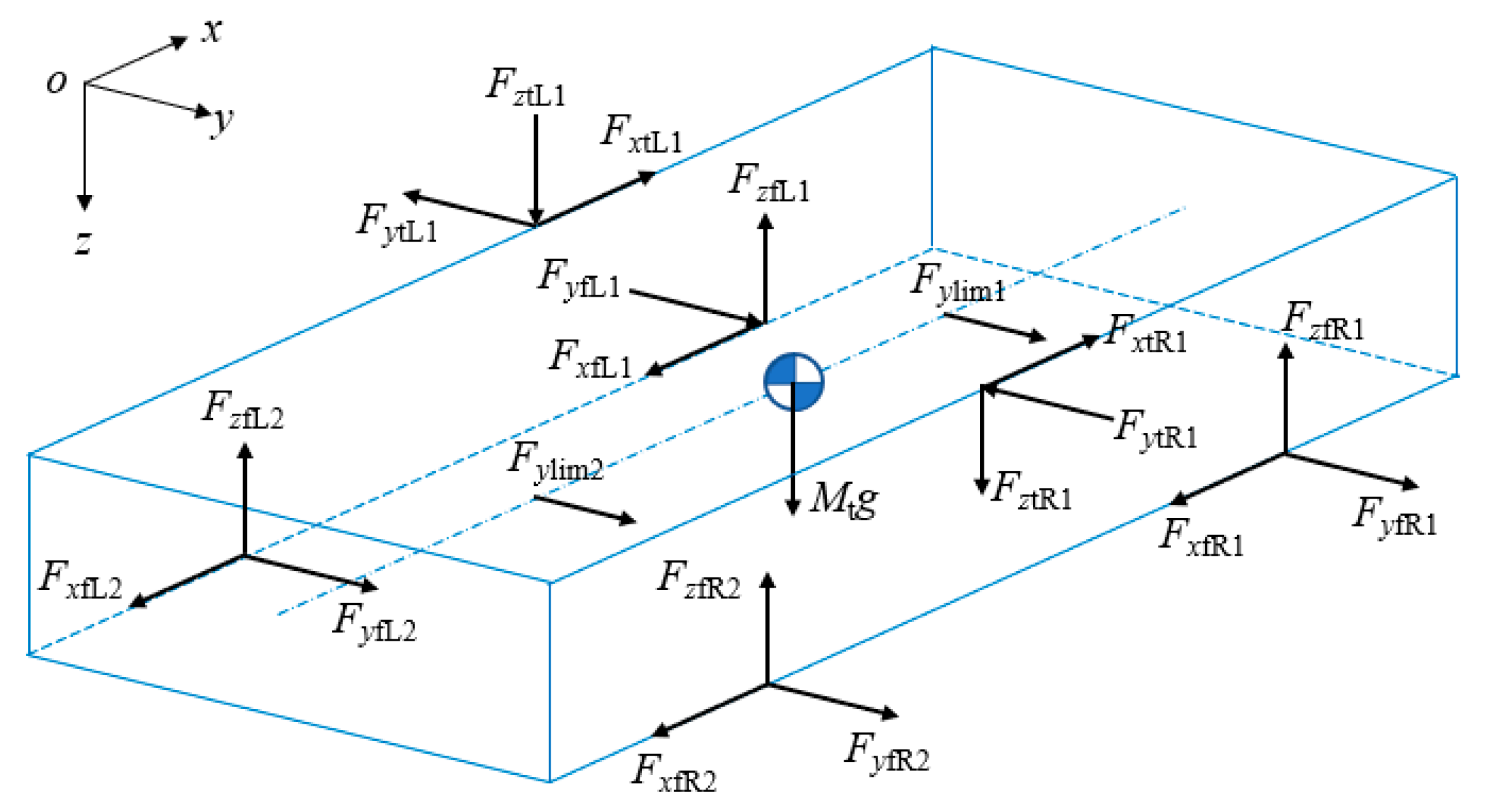
2.1.1. Vehicle System

The vehicle system was simplified into one car body, two bogie frames, and four wheelsets, each part of which was regarded as rigid body. The LIM was simplified into Euler beam. All parts are connected through the vehicle suspension system and simulated by a spring-damping connection unit. The degree of freedom contained in the LIM vehicle system is shown in Table 1.
Force analysis is carried out on each vehicle component, as shown in Figure 3, Figure 4 and Figure 5. Based on the force analysis, motion differential equations of each part are established.
Equation of car body motion:
Longitudinal motion:
M c X ¨ c = F x tL 1 F x tR 1 F x tL 2 F x tR 2 F x cf F x cb
Lateral motion:
M c Y ¨ c + v 2 R c + r 0 + H tw + H Bt + H cB ϕ ¨ sec = F y tL 1 + F y tR 1 + F y tL 2 + F y tR 2 F x cf F x cb + M c g ϕ sec
Vertical motion:
M c Z ¨ c a 0 ϕ ¨ sec v 2 R c ϕ sec = F z tL 1 F z tR 1 F z tL 2 F z tR 2 F z cf F z cb + M c g
Swing motion:
I c x ϕ ¨ c + ϕ ¨ sec = F y tL 1 + F y tR 1 + F y tL 2 + F y tR 2 H cB + F z cf + F z cb H cc + F z tL 1 F z tR 1 + F z tL 2 F z tR 2 d s M x s 1 M x s 2
Nodding motion:
I c y β ¨ c = F z tL 1 + F z tR 1 F z tL 2 F z tR 2 l c F x tL 1 + F x tR 1 + F x tL 2 + F x tR 2 H cB + F z cf F z cb l cc F x cf + F x cb H cc
Yaw motion:
I c z ψ ¨ c + v d d t 1 R c = F y tL 1 + F y tR 1 F y tL 2 F y tR 2 l c + F x tL 1 + F x tR 1 F x tL 2 + F x tR 2 d s + F y cf F y cb l cc
Equation of bogie frame motion (i = 1~2):
Longitudinal motion:
M t X ¨ t i = F x fL 2 i 1 F x fR 2 i 1 F x fL 2 i F x fR 2 i + F x tL i + F x tR i
Lateral motion:
M t Y ¨ t i + v 2 R t i + r 0 + H tw ϕ ¨ set i = F y fL 2 i 1 + F y fL 2 i + F y fR 2 i 1 + F y fR 2 i F y tL i F y tR i + F y lim 1 + F y lim 2 + M t g ϕ set i
Vertical motion:
M t Z ¨ t i a 0 ϕ ¨ set i v 2 R t i ϕ set i = F z tL i + F z tR i F z fL 2 i 1 F z fR 2 i 1 F z fL 2 i F z fR 2 i + M t g
Swing motion:
I t x ϕ ¨ t i + ϕ ¨ set i = F y fL 2 i 1 + F y fR 2 i 1 + F y fL 2 i + F y fR 2 i H tw + F z fL 2 i 1 F z fR 2 i 1 + F z fL 2 i F z fR 2 i d w + F z tR i F z tL i d s F y tL i + F y tR i H Bt + M x s i
Nodding motion:
I t y β ¨ t i = F z fL 2 i 1 + F z fR 2 i 1 F z fL 2 i F z fR 2 i l t F x fL 2 i 1 + F x fR 2 i 1 + F x fL 2 i + F x fR 2 i H tw F x tL i + F x tR i H Bt
Yaw motion:
I t z ψ ¨ t i + v d d t 1 R t i = F y fL 2 i 1 + F y fR 2 i 1 F y fL 2 i F y fR 2 i l t + F y lim 1 F y lim 2 l lim + F x fR 2 i 1 + F x fR 2 i F x fL 2 i 1 F x fL 2 i d w + F x tL i F x tR i d s
Equation of wheelset motion (i = 1~4):
Longitudinal motion:
M w X ¨ w i = F x fL i + F x fR i N L x i N R x i F L x i F R x i
Lateral motion:
M w Y ¨ w i + v 2 R w i + r 0 ϕ ¨ sew i = F y fL i F y fR i + F L y i + F R y i + N L y i + N R y i
Vertical motion:
M w Z ¨ w i a 0 ϕ ¨ sew i v 2 R w i ϕ sew i = F z fLi + F z fRi F L z i F R z i N L z i N R z i + F z lim i + M w g
Swing motion:
I w x ϕ ¨ sew i + ϕ ¨ w i I w y β ˙ w i Ω ψ ˙ w i + v R w i = a 0 F L z i + N L z i F R z i N R z i r L i F L y i + N L y i r R i F R y i + N R y i + d w F z fR i F z fL i
Nodding motion:
I w y β ¨ w i = r R i F R x i + r L i F L x i + r R i ψ w i F R y i + N R y i + r L i ψ w i F L y i + N L y i + M L y i + M R y i + N L x i r L i + N R x i r R i
Yaw motion:
I w z ψ ¨ w i + v d d t 1 R w i I w y ϕ ˙ sew i + ϕ ˙ w i β ˙ w i Ω = M L z i + M R z i + d w F x fL i F x fR i + a 0 F L x i F R x i + a 0 N L x i N R x i + a 0 ψ w i F L y i + N L y i F R y i N R y i
where Mc, Mt, Mw are the mass of the vehicle body, frame, and wheelset, respectively. Icx, Icy, Icz are the moment of inertia of the vehicle body around x, y, and z axes, respectively. Itx, Ity, Itz are the moment of inertia of the bogie frame around x, y, and z axes, respectively. Iwx, Iwy, Iwz are the moment of inertia of the wheelset around x, y, and z axes, respectively. Rc, Rti (i = 1~2), Rwi (i = 1~4) are, respectively, the radius of curvature corresponding to the car body, the i-th bogie, and the i-th wheelset center. ϕsec, ϕseti (i = 1~2), ϕsewi (i = 1~4) are, respectively, the outer rail elevation angle corresponding to the car body, the i-th bogie, and the i-th wheelset center. r0 is the nominal radius of wheel rolling circle, a0 is half of the distance between left and right wheel contact points, dw and ds is half of the transverse distance between the suspension of series 1 and 2, lc and lt is half of the distance between the vehicle and the bogie, Htw is the vertical distance between the frame center of mass and the center line of wheelset. HcB is the distance between the vehicle body center of mass and secondary suspension upper surface. HBt is the distance between the frame center of mass and secondary suspension lower surface. rji (j = L, R, i = 1~4) is the rolling radius of the left wheel and right wheel of the i-th wheelset. Fxfji, Fyfji, Fzfji (j = L, R, i = 1~4) are the primary suspension force of i-th wheelset. Fxsji, Fysji, Fzsji (j = L, R, i = 1~4) are the secondary suspension force of i-th wheelset. Njxi, Njyi, Njzi (j = L, R, i = 1~4), respectively, are the normal force of the i-th wheelset. Fjxi, Fjyi, Fjzi (j = L, R, i = 1~4) are the creep force of the i-th wheelset respectively. Mjxi, Mjyi, Mjzi (j = L, R, i = 1~4) are the creep moment of the i-th wheelset, Mxsi (i = 1~2) is the anti-roll moment of the i-th frame. Fylim, Fzlim are the transverse and vertical pull rod force of the LIM. llim is the half distance between the two axles of suspending LIM.
And the key parameters of the vehicle are listed in Table 2.

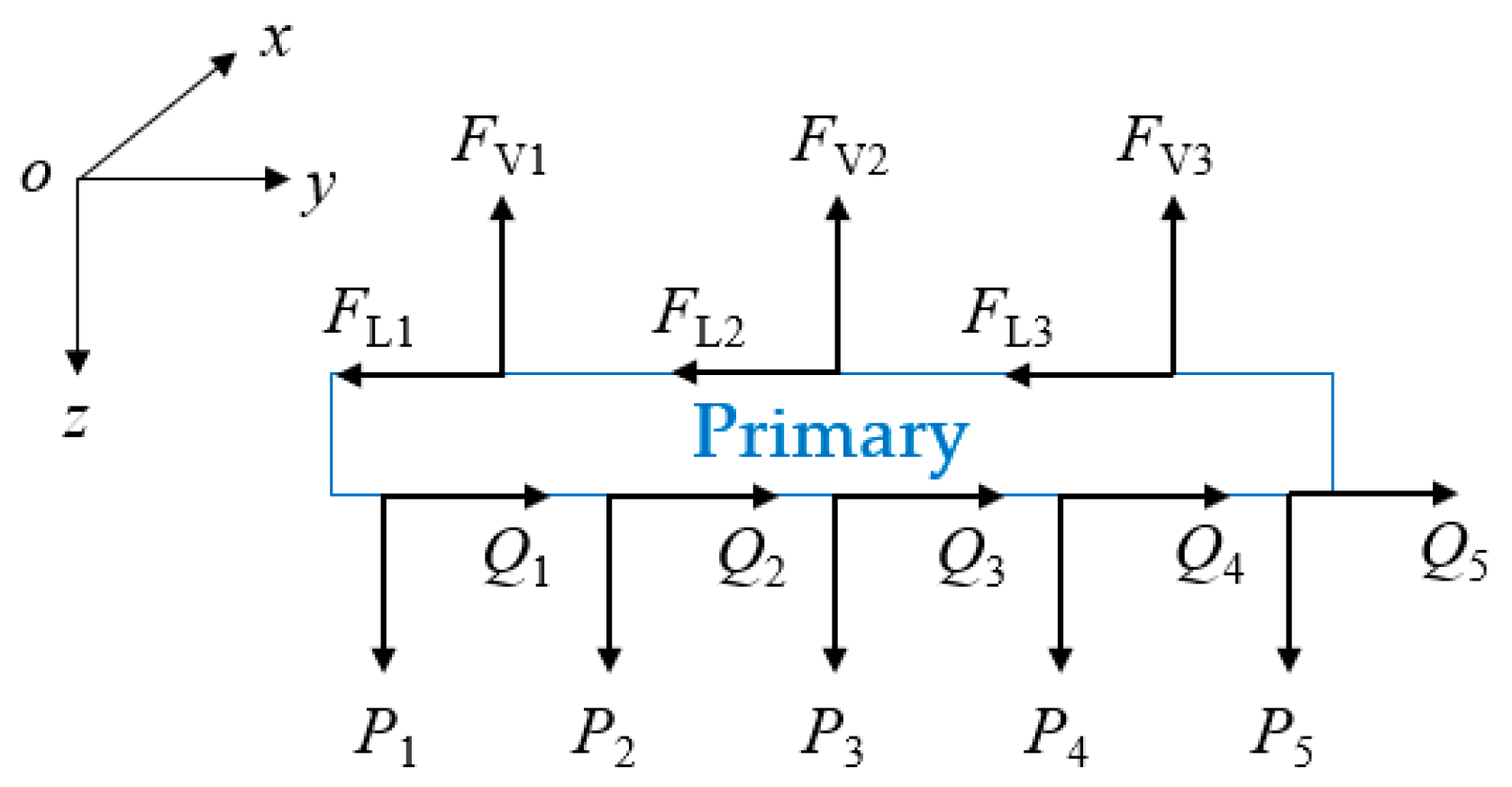
2.1.2. Primary Winding Vibration Differential Equation

The primary winding is suspended from the front and rear axles of the bogie by five suspenders. An Euler beam with the “free-free” boundary condition is used to simulate the transverse and vertical vibrations of the primary winding. The boom is simulated by a spring damping unit.
The force analysis of the primary winding is shown in Figure 6. And based on the force analysis, motion differential equations are established.
E d I Z d 4 Y d x , t x 4 + m d 2 Y d x , t t 2 = i L I M = 1 N L I M Q j x , t δ x x i L I M L i = 1 3 F L j , x δ x x L i E d I Y d 4 Z d x , t x 4 + m d 2 Z d x , t t 2 = i L I M = 1 N L I M P j x , t δ x x i L I M L i = 1 3 F V j , x δ x x L i
where Ed and md are the equivalent elastic modulus and mass of the primary, respectively; IZd and IYd are the cross-sectional moments of inertia of the primary; Yd and Zd are the transverse and vertical displacements of the primary, respectively; FL and FV are the forces of the transverse tie rod and vertical boom, respectively; P and Q are the transverse and vertical electromagnetic forces, respectively; and xiLIM is the position of the electromagnetic force between the primary and secondary conductive plate.

2.1.3. Vehicle End Connection System Model

The vehicle end connection system consists of a coupler and draft gear, which have strong nonlinear characteristics. We simplify it to a force element simulation with a segmented linear stiffness, as shown in Figure 7.
This force element can be expressed as
F cg = 0 , Δ x < Δ x 0 , K CB 1 Δ x Δ x 0 , Δ x 0 Δ x x 0 CB , K CB 1 x 0 CB Δ x 0 + K CB 2 Δ x x 0 CB , Δ x x 0 CB ,
Δ x = x cf x cb 2 + y cf y cb 2 + z cf z cb 2 L 0
where ∆x0 is the free clearance of the coupler draft gear, x0CB is the length of the primary stiffness for the coupler draft gear, KCAB1 and KCAB2 are the equivalent stiffness of the coupler draft gear, L0 is the initial equivalent length of the coupler draft gear, xcf, ycf, and zcf are the spatial coordinates of the coupler connection point connected to the front car, and xcb, ycb, and zcb are the spatial coordinates of the coupler connection point connected to the rear car.

2.2. Track System

2.2.1. Rail System

The rail is considered as a Timoshenko beam with “simply supported-simply supported” boundary conditions. The equations of motion in the transverse, vertical, and torsional directions are shown.
Lateral motion:
m 2 y x , t t 2 + κ y G A ψ y x , t x 2 y x , t x 2 = i = 1 N s R y i t δ x x s i + j = 1 N w F wr y i t δ x x w j ρ I z 2 ψ y x , t t 2 + κ y G A ψ y x , t y x , t x E I z 2 ψ y x , t x 2 = 0  
Vertical motion:
m 2 z x , t t 2 + κ z G A ψ z x , t x 2 z x , t x 2 = i = 1 N s R z i t δ x x s i + j = 1 N w F wr z i t δ x x w j ρ I y 2 ψ z x , t t 2 + κ z G A ψ z x , t z x , t x E I y 2 ψ z x , t x 2 = 0  
Twisting motion:
ρ I 0 2 ϕ x , t t 2 G K 2 ϕ x , t x 2 = i = 1 N s M s i t δ x x s i + j = 1 N w M G j t δ x x w j  
where y, z and ϕ are the transverse, vertical and torsional displacements of the rail. ψz and ψy are the angular deformation of the rail cross section on z and y axles, respectively. Ryi and Rzi are the lateral and vertical reaction forces of the i-th fulcrum. Fwryj and Fwrzj are the transverse and vertical loads of the jth wheel on the rail, respectively. Msi and MGj are the moment of reaction force of the of the ith rail and the jth wheel on the rail. Iy and Iz are the inertia moment of rail cross section on y and z axles. G is the rail shear modulus. A is the cross-sectional area of the rail. Ns is the number of fasteners within the calculation area. Nw is the number of wheelsets. While κy and κz are shear factors of rail transverse and vertical cross section, the values are 0.4507 and 0.532.
The vibration response of the rail is analyzed by separation variable method. Regular mode shape function and regular coordinates represent the transverse, vertical, and torsional displacement. First, the rail vibration partial differential equation is simplified into a second-order ordinary differential equation about the regular mode coordinates, by using the orthogonality of the regular mode and the properties of the Dirichlet function. Then, find the canonical coordinates by the rail boundary. Finally, the transverse, vertical, and torsional displacements of the rail are obtained by multiplying and superimposing with the regular mode function and the canonical coordinates.

2.2.2. Secondary Conductive Plate Vibration Differential Equation

The secondary conductive plate is fixed on the centre of the track plate by fasteners, as shown in Figure 2. A Euler beam with the “simply supported-simply supported” boundary condition is used to simulate the transverse vertical and torsional vibrations of the secondary conductive plate. The fasteners fixing the secondary conductive plate are simulated by a spring damping unit. The force analysis of the secondary conductive plate is shown in Figure 8. And based on the force analysis, motion differential equations are established.
E p I Z p 4 Y P ( x , t ) x 4 + m p 2 Y P ( x , t ) t 2 = i = 1 n F LRP i ( t ) δ ( x x i ) + j = 1 2 i L I M N L I M Q j ( x , t ) δ ( x x i L I M ) E p I Yp 4 Z P ( x , t ) x 4 + m p 2 Z P ( x , t ) t 2 = i = 1 n F LRP i ( t ) δ ( x x i ) + j = 1 2 i L I M N L I M P j ( x , t ) δ ( x x i L I M )
where Ep and mp are the equivalent elastic modulus and mass per unit length of the secondary conductive plate, respectively; IZp and IYp are the cross-sectional moments of inertia of the secondary conductive plate; Yp and Zp are the transverse and vertical displacements of the secondary conductive plate, respectively; FLRPi and FVRPi are the forces of the track plate on the secondary conductive plate; Q and P are the transverse and vertical electromagnetic forces, respectively; and xi is the position of the secondary conductive plate fastener pivot point.

2.3. Wheel-Rail Interaction System

2.3.1. Wheel-Rail Spatial Contact Geometry Model [17,18]

The wheel traces are generated from the motion parameters of the wheelset and the tread profile, and the new rail profile is generated by the motion parameters of the rail and the rail profile. Then the minimum vertical distance between the wheel traces and the new rail profile is found as the wheel-rail contact point by transverse scanning. As the wheels run, the motion parameters of the wheels and rails change, which affects the wheel traces and the new rail profile, and thus the position of the wheel-rail contact point.

2.3.2. Normal Force Calculation Model

The wheel-rail normal force is solved by the Hertz nonlinear elastic contact theory, and the calculation formula is shown in Equation (26).
N t = 1 G wr Z wrnc ( t ) 3 / 2 , Z wmc ( t ) > 0 0 , Z wmc ( t ) 0
where, Gwr is the wheel-rail contact constants (m/N3/2). Which can be obtained by Hertz contact theory [19], and the value can be [20]
Gwr = 3.86R−0.115 × 10⁻⁸
where, R is the rolling distance of the wheel. Zwrnc (t) represents the normal elastic compression of wheel-rail contact point. When the value of Zwrnc (t) is less than zero, it means the wheel and rail separated, and the wheel-rail normal force is zero.

2.3.3. Creep Force Calculation Model

Firstly, the calculations were carried out according to the Kalker theory [21]. When the creep between the wheel and rail saturation, the Shen-Hedrick-Elkins theory [22] is used for nonlinear correction. Considering the effects of transverse, vertical, and torsional motions of the left and right rails on the creep-slip rate of wheel-rail rolling contact, the wheel-rail creep-slip rate is obtained according to the wheel-rail spatial contact geometry relationship as:
ξ k x = V w x V r x V ξ k y = V w y V r y V ξ k n = V w n V r n V
where, V represents the nominal forward speed of the wheelset on the rail. Vwx, Vwy, Vwn are velocity components of the wheel in contact the spot coordinate system in x, y, and z directions. Vrx, Vry, Vrn are velocity components of the rail in contact the spot coordinate system in x, y, and z directions.
The creep force between wheel and rail can be expressed as:
F x k = f 11 ξ k x F y k = f 22 ξ k y f 23 ξ k n M n k = f 23 ξ k y f 33 ξ k n
where, Fxk, Fyk, Mnk are the longitudinal creep force, transverse creep force, and spin creep motion of the kth wheel, respectively. ξkx, ξky, ξkn represent the longitudinal, transverse, and spin creep rate at the kth wheel, respectively. f11, f22, f33, f23 represent the longitudinal, transverse, spin creep coefficients, and spin/transverse creep coefficients, respectively.
As the Kalker linear creep theory is only suitable for small creep rates and small spins, the Shen-Hedrick-Elkins is used for correction [20]. The friction force between wheel and rail at the kth wheel can be expressed as:
F f k = f P wrn k
where, f represents the friction coefficient between wheel and rail. And Pwrnk is the wheel-rail normal force on kth wheel.
Combine the creep force of longitudinal and transverse obtained by Kalker linear creep theory as:
F R k = F x k 2 + F y k 2
Let:
F R k = F f k F R k F f k 1 3 F R k F f k 2 + 1 27 F R k F f k 3 , F R k 3 F f k F f k , F R k > 3 F f k
Introduce correction coefficient:
ε = F R k F R k
The expressions of creep force and creep torque obtained by Shen-Hedrick-Elkins theory are as follows:
F x k = ε F x k F y k = ε F y k M n k = ε M n k

2.4. Electromagnetic Interaction System

When the primary winding is energised, a traveling magnetic field occurs between the primary winding and secondary conductive plate, and a corresponding induction current is generated in the secondary conductive plate. The induction current cuts the magnetic induction lines of the traveling magnetic field and generates an electromagnetic force, which drives the train.
To facilitate the numerical calculation, the transverse and vertical electromagnetic forces are simplified into curves in the coupled train-track system dynamic model, as shown in Figure 9.

3. Operational Safety Evaluation Criteria

According to the derailment mechanism, derailment types can be divided into wheel climb, slipway, and overturning derailments. Owing to the low speed of the train on the yard line, there is no jumping derailment, so that we focus on wheel climb and overturning derailments.

3.1. Derailment Coefficient

According to GB/T 14894-2005 “Rules for Inspection and Testing of Urban Rail Transit Vehicles After Assembly”, the limit value of the derailment coefficient for a wheel climb derailment is 0.8.
Q P < 0.8
where Q and P are the wheel-rail transverse and vertical forces, respectively.
This standard considers wheel climb derailment as occurring at the moment when the wheel-rail derailment coefficient exceeds the limit. However, in practice, the wheel climb derailment is a dynamic process. Therefore, Japan Railway Institute of General Technology proposed a derailment coefficient exceeding 0.8 for a duration of 15 ms as a wheel climb derailment judging criterion [23]. If the derailment coefficient exceeds 0.8 for a duration shorter than 15 ms, the operation is considered safe; otherwise, a derailment occurs. In this study, the derailment safety of the train is judged according to this criterion.

3.2. Wheel Unloading Rate

The wheel unloading rate is defined as the ratio of wheel unloading on the reduced load side to the average wheel weight on both sides of the wheel pair. Its safety standard is 0.6.
Δ P P 0.6
where ΔP and P are the wheel load reduction and average wheel load, respectively. GB/T 14894-2005 “Rules for Inspection and Testing of Urban Rail Transit Vehicles After Assembly” stipulates that the wheel unloading rate is used to assess whether the wheels derail due to an excessive reduction in load on one side of the wheels.

3.3. Axle Lateral Force

To avoid an excessive axle transverse force leading to a dynamic instability of the line resulting in an expansion of the track or transverse slip, GB/T 5599-2019 “Rolling Stock Dynamic Performance Assessment and Test Identification Specification” stipulates that the axle transverse force should comply with
H 15 + P 0 3
where H is the axle transverse force and P0 is the static axle weight.

4. Derailment Safety and Speed Limit Analysis

4.1. Conventional Conditions

As the yard line is often designed with an S-curve, we use the line shown in Figure 10, where the radius of the circular curve is 65 m. The radius of the curve turning to the right is defined as positive, while the opposite is negative.
Because of the low speed of trains running on the yard line (usually below 25 km/h), the yard line usually is not set ultra-high. The wheel-rail contact exhibits the profile of a new wheel and new rail, with the US five-level spectrum excitation.
When the train runs at a speed of 25 km/h on the yard line, the attack angle of the wheelset and derailment coefficient of the first wheelset of the first vehicle are calculated, as shown in Figure 11a,b, respectively. When the wheelset has a counter clockwise angle of rotation with respect to the track, the defined attack angle is positive, while a clockwise angle is negative, as shown in Figure 12.
Figure 11a shows that when the wheelset passes the first curve of the S-shaped curve, the angle attack of the wheelset is positive, while the angle attack is negative when it passes the second curve. Figure 11b shows that, at this time, the wheelset derailment coefficient is seriously overrun, i.e., the wheelset has a tendency to climb the rail at this time so that it is necessary to strictly control the time when the derailment coefficient exceeds the limit to avoid a derailment. Thus, the duration of derailment coefficient overrun is chosen as a derailment criterion in this study.
Figure 13 shows that the maximum static derailment coefficient of each car exceeds the static derailment limit of 0.8. The maximum value occurs when the vehicle passes through the straight point of the curve.
Figure 14 shows time-domain simulation results of the maximum value of the derailment coefficient for each car under these operation conditions and statistical results of the duration of derailment coefficient overrun. The duration of derailment coefficient overrun exceeds the safety limit (15 ms) for the 1st axle of the 3rd car and the 1st axle of the 6th car. Therefore, a climbing derailment occurs when the train runs on the entry line at a speed of 25 km/h. Statistical results of subway vehicle derailment accidents of subway vehicles on the yard line also demonstrated that the middle car of the train derails first (often the third car).
To determine the speed safety limit of the train running on the yard line, Figure 15 shows statistical results of the derailment coefficient, axle lateral force, duration of derailment coefficient overrun, and wheel unloading rate for trains running through the yard line at speeds of 5 to 25 km/h.
As shown in Figure 15a, the changes in the derailment coefficient and axle lateral force with the decrease in the speed are small, but both seriously exceed the safety limits. Figure 15b shows that when the speed is below 20 km/h, the duration of derailment coefficient overrun decreases with the decrease in the speed, and is within the safety limit. In addition, the wheel unloading rate decreases with the decrease in the speed, and is within the safety limit when the speed is below 25 km/h. According to this criterion, when the train passes on the yard line at a speed below 20 km/h, there would be no wheel climb derailment and overturning derailment.
To illustrate the reason for the overrun of the axle lateral force, Figure 16 shows the changes in the wheel/rail lateral force and axle lateral force of the 1st axle of the 1st car in the time domain when the train passes the yard line at a speed of 25 km/h.
As shown in Figure 16, when the train passes through the first circular curve of the S-curve (rightward) at a speed of 25 km/h, the lateral force of the left wheel increases sharply. At the outer rail (left rail) side, the wheel flange face contacts with the rail gauge face, which increases the wheel-rail contact angle and lateral component of the wheel-rail force. Similarly, when the train passes the second circular curve of the S-curve (leftward), at the outer rail (right rail) side, the wheel flange face contacts with the rail gauge face, which increases the wheel-rail lateral force sharply. Considering Figure 15a, under this condition, the lateral force of the axle does not decrease significantly with the decrease in the speed, which indicates that the lateral force of the axle is less affected by the train speed than by the small-radius curve of the line.
In summary, when the LIM subway vehicle passes through the yard line at a speed of 5 to 25 km/h, the wheel-rail system is in the new wheel-new rail matching state, and their friction coefficients are set to 0.3. When the derailment coefficient and axle lateral force safety seriously exceeded the safety limits, the numerical results of the simulation did not characterise the derailment of the train. However, the wheel-rail rolling contact state must be close to the boundary state of the derailment. Over the years of field operations, incidents of wheel climb derailment are still a minority. In this regard, the critical point of safety redundancy of wheel climb derailment is of interest to be further investigated.

4.2. Wheel-Rail Extreme Wear Conditions

As mentioned in the previous section, due to the limitation of the small radius of the curve, the wheel flange face contacts with the rail gauge face seriously in the circular curve section, which leads to a serious wheel-rail wear. The wheel-rail wear profile affects the wheel-rail contact relationship, thus affecting the traffic safety. Therefore, it is also necessary to study the traffic safety and speed limits of trains running through the yard line under the conditions of wheel rail wear.
The worn rail profile used in this section is the actual measured profile of an overused rail on the yard line, as shown in Figure 17a. In the calculation analysis, the worn rail profile is used for the outer rail of the curve, and the new rail profile is used for the inner rail. The worn wheel profile is obtained from the worn wheel profile for running for 100,000 km after turning, as shown in Figure 17b.
Figure 18 shows the statistics of the maximum values of the derailment coefficient, axle lateral force, duration of the derailment coefficient, and wheel unloading rate of the LIM trains running through the yard line at a speed of 25 to 5 km/h.
Figure 18a shows that the changes in the derailment coefficient and axle lateral force with the decrease in the speed are small. At a speed of 5 to 25 km/h, the derailment coefficient is within the safety limit, while the lateral axle force exceeds the safety limit. Figure 18b shows that the duration of derailment coefficient overrun decreases with the decrease in the speed, and is within the safety limit. As the derailment coefficients are within the safety limit, the durations of derailment coefficient overrun are 0. Therefore, the LIM train does not derail when it passes through the yard line under this condition. When the wheel and rail are seriously worn, LIM trains can more easily run through the yard line, because the wheel diameter difference of the worn wheel-worn rail matching is significantly larger than that of the new wheel-new rail matching. Figure 19 gives the wheel diameter difference comparison of the 1st axle of the 1st car of the worn wheel-worn rail matching and new wheel-new rail matching. The wheel diameter difference changes the alignment balance of the wheelsets. So, the larger wheel diameter difference results in a significant improvement in the train’s curve passing performance.
Further, we consider the operation safety of trains running through the yard line under conditions of a seriously worn track and new wheel matching. The derailment factor, axle lateral force, and wheel unloading rate were not significantly different (slightly improved) from the results of the new wheel-rail matching (Figure 15). Therefore, the results are not repeated here. The duration of derailment coefficient overrun under the conditions of worn rail-new wheel matching is presented in Figure 20.
As shown in Figure 20, the derailment factor overrun time decreases with the decrease in the speed in the range of 5 to 25 km/h. When the speed is below 15 km/h, the derailment factor overrun time is within the safety limit. Thus, under this condition, there will be no wheel climb derailment. The comparison of Figure 15b and Figure 20 shows that the worn rail reduces the safety when the train passes through the yard line.

5. Conclusions

The operational safety and speed limit of LIM trains running through an inbound- outbound line were studied through the established LIM subway train-track (including the secondary conductive plate) coupled dynamic six-group model. When the LIM train passes through the yard line at a speed below 25 km/h, for both new wheel matchings with the new rail and worn rail, the changes in the derailment coefficient and axle lateral force with the decrease in the speed were small, but both seriously exceeded the safety limits. This indicates that trains are prone to wheel climb derailment on the yard line. However, the wheel unloading rate is within the safety limit, so that the overturning derailment will not occur. When the extremely worn wheel was matched with the extremely worn rail, the derailment coefficient and wheel unloading rate of the train changed slightly with the decrease in the speed, and were within the safety limits. This indicated that wheel climb and overturning derailments will not occur. When the train passes through the yard line, only the worn rail has a small effect on the safety of the train, while the matching of extremely worn rails and worn wheels improves the safety of the train.
Under the conditions considered in this study, the numerical simulation results do not indicate a wheel climb derailment when the train passes through the yard line. The redundancy of the critical point where the wheel climbing occurs is unclear and needs to be further investigated by developing more accurate models and corresponding numerical methods. More influencing factors need to be considered, including the change in the friction coefficient of the wheel-rail interface, geometric irregularities, small turnouts, and sudden changes in support stiffness. In the case where the LIM trains run through the yard line in a state similar to that discussed in this paper, it is recommended that the train passing speed should be below 15 km/h.

Author Contributions

Methodology, Q.Z.; Software, J.W. and J.H.; Investigation, X.J.; Writing—original draft, Q.Z.; Writing—review & editing, X.J. All authors have read and agreed to the published version of the manuscript.

Funding

This study was supported by the National Natural Science Foundation of China (U1734201).

Institutional Review Board Statement

This thesis does not involve human or animal research.

Informed Consent Statement

This thesis does not involve human or animal research.

Data Availability Statement

Data available on request due to restrictions eg privacy or ethical. The data presented in this study are available on request from the corresponding author. The data are not publicly available due to the request of the metro operator.

Conflicts of Interest

The authors declare no conflict of interest.

References

  1. Bollinger, C.R.; Ihlanfeldt, K.R. The Impact of Rapid Rail Transit on Economic Development: The Case of Atlanta’s MARTA. J. Urban Econ. 1997, 42, 179–204. [Google Scholar] [CrossRef]
  2. Hellinger, R.; Mnich, P. Linear Motor-Powered Transportation: History, Present Status, and Future Outlook. Proc. IEEE 2009, 97, 1892–1900. [Google Scholar] [CrossRef]
  3. Zeng, H. Advantages and application of linear induction motor in urban transit system. Convert. Technol. Electr. Tract. 2008, 4, 51–53, 59. [Google Scholar]
  4. Lv, G. Review of the Application and Key Technology in the Linear Motor for the Rail Transit. Proc. CSEE 2020, 40, 5665–5675. [Google Scholar]
  5. Isobe, E.; Cho, J.; Morihisa, I.; Sekizawa, T.; Tanaka, R. Linear metro transport systems for the 21st century. Hitachi Rev. 1999, 48, 144–148. [Google Scholar]
  6. Li, N. Characteristics and application of linear motor driven urban mass transit system. Electr. Locomot. Mass Transit Veh. 2005, 28, 3–52. [Google Scholar]
  7. Hobbs, A.E.W.; Pearce, T.G. The lateral dynamics of the linear induction motor test vehicle. J. Dyn. Syst. J. Dyn. Syst. Meas. Control 1974, 96, 147–157. [Google Scholar] [CrossRef]
  8. Feng, Y.W.; Wei, Q.C.; Gao, L.; Shi, J. Dynamic simulation of vehicle-track coupling vibrations for linear metro system. In Environmental Vibrations: Prediction, Monitoring, Mitigation and Evaluation (ISEV 2005); CRC Press: Boca Raton, FL, USA, 2021; pp. 131–136. [Google Scholar]
  9. Li, L. Study on Spatial Coupling Dunamic Characteristics of Vechicle-Turnout in Linear Induction Motor Wheel/Rail Traffic System. Ph.D. Thesis, Beijing Jiaotong University, Beijing, China, 2009. [Google Scholar]
  10. Li, L.; Xiao, X.B.; Jin, X.S. Interaction of subway LIM vehicle with ballasted track in polygonal wheel wear development. Acta Mech. Sin. 2011, 27, 297–307. [Google Scholar]
  11. Liu, G. Influence of Electromagnetic Force on the Dynamic Performance of Linear Motor Metro Vehicle. Master’s Thesis, Southwest Jiaotong University, Chengdu, China, 2015. [Google Scholar]
  12. Jang, S.M.; Park, Y.S.; Sung, S.Y.; Lee, K.B.; Cho, H.W.; You, D.J. Dynamic characteristics of a linear induction motor for predicting operating performance of magnetic levitation vehicles based on electromagnetic field theory. IEEE Trans. Magn. 2011, 47, 3673–3676. [Google Scholar] [CrossRef]
  13. Xiong, J.Y. Study on Dynamic Response of Linear Motor Metro Vehicle Coupled with Slab Track. Ph.D. Thesis, South West Jiaotong University, Chengdu, China, 2014. [Google Scholar]
  14. Liu, B.B.; Zheng, J.; Luo, R.; Wu, P.B. Modeling and dynamics simulation of vehicle with linear induction motor. J. Traffic Transp. Eng. 2009, 9, 37–43. [Google Scholar]
  15. Yang, Y.F. Study on Dynamic Interactions of Linear Motor Metro Vehicle Coupled with Track. Master’s Thesis, Southwest Jiaotong University, Chengdu, China, 2017. [Google Scholar]
  16. Zang, C.Z.; Wei, Q.C.; Nie, X.L. Dynamic response of the LIM wheel/rail train in curved section. J. Harbin Inst. Technol. 2019, 51, 110–116. [Google Scholar]
  17. Chen, G.; Zhai, W.M.; Zuo, H.F. The New Wheel/Rail 3-Dimensionally Dynamically Coupling Model. J. Vib. Eng. 2001, 14, 402–408. [Google Scholar]
  18. Chen, G.; Zhai, W.M. A New Wheel Rail Spatially Dynamic Coupling Model and its Verification. Veh. Syst. Dyn. 2004, 41, 301–322. [Google Scholar] [CrossRef]
  19. Jin, X.S.; Liu, Q.Y. Tribology of Wheel and Rail; China Railway Publishing House: Beijing, China, 2004. [Google Scholar]
  20. Zhai, W.M. Vehicle-Track Coupled Dynamics, 4th ed.; Science Press: Beijing, China, 2015. [Google Scholar]
  21. Kalker, J.J. On the rolling Contact of Two Elastic Bodies in the Presence of Dry Friction. Ph.D. Thesis, Delft University, Delft, The Netherland, 1967. [Google Scholar]
  22. Shen, Z.Y.; Hedrick, J.K.; Elkins, J.A. A comparison of alternative creep force models for rail vehicle dynamic analysis. Veh. Syst. Dyn. 1983, 12, 79–83. [Google Scholar] [CrossRef]
  23. Ishida, H.; Matsuo, M. Safety criteria for evaluation of railway vehicle derailment. Q. Rep. RTRI 1999, 40, 18–25. [Google Scholar] [CrossRef] [Green Version]
Figure 1. Photograph of a subway yard line.
Applsci 13 04163 g001
Figure 2. LIM subway vehicle-track coupling dynamic six-group model.
Applsci 13 04163 g002
Figure 3. Force analysis of car body.
Applsci 13 04163 g003
Figure 4. Force analysis of car bogie frame.
Applsci 13 04163 g004
Figure 5. Force analysis of wheelset.
Applsci 13 04163 g005
Figure 6. Force analysis of the primary winding.
Applsci 13 04163 g006
Figure 7. Coupler draft gear device force element.
Applsci 13 04163 g007
Figure 8. Force analysis of the secondary conductive plate.
Applsci 13 04163 g008
Figure 9. Electromagnetic force curve [15].
Applsci 13 04163 g009aApplsci 13 04163 g009b
Figure 10. Line setting.
Applsci 13 04163 g010
Figure 11. Attack angle and derailment coefficient: (a) attack angle of the wheelset; (b) derailment coefficient.
Applsci 13 04163 g011
Figure 12. Attack angle diagram.
Applsci 13 04163 g012
Figure 13. Derailment coefficient time-domain diagram.
Applsci 13 04163 g013
Figure 14. Statistical results of the duration of derailment coefficient overrun.
Applsci 13 04163 g014
Figure 15. Operation safety indices vs. train running speed under conventional condictions: (a) derailment coefficient and axle lateral force; (b) duration of derailment coefficient overrun and wheel unloading rate.
Applsci 13 04163 g015
Figure 16. Wheel-rail lateral force and axle lateral force in the time domain.
Applsci 13 04163 g016
Figure 17. Wear profile: (a) worn rail profile; (b) worn wheel profile.
Applsci 13 04163 g017
Figure 18. Operation safety indices vs. train running speed under extreme wear conditions: (a) derailment coefficient and axle lateral force; (b) duration of derailment coefficient overrun and wheel unloading rate.
Applsci 13 04163 g018
Figure 19. Wheel diameter difference.
Applsci 13 04163 g019
Figure 20. Duration of derailment coefficient overrun vs. train running speed.
Applsci 13 04163 g020
Table 1. Degree of freedom contained in the LIM vehicle system.
Degree of FreedomLongitudinalLateralVerticalSwingNoddingYaw
Car bodyXcYcZcΦcβcΨc
Bogie frames (i = 1~2)XtiYtiZtiΦtiβtiΨti
Wheelsets (i = 1~4)XwiYwiZwiΦwiβwiΨwi
Table 2. The key parameters of the vehicle.
Vehicle ComponentsValue (Unit)
Mc42.8 (t)
Mt1.1 (t)
Mw1.0 (t)
Icx, Icy, Icz51.0, 986.3, 988.0 (t·m2)
Itx, Ity, Itz1.1, 0.4, 1.0 (t·m2)
Iwx, Iwy, Iwz0.6, 0.1, 0.6 (t·m2)
Primary suspension stiffness (x, y and z axes)5.2, 5.2, 1.2 (kN/mm)
Primary suspension damping (x, y and z axes)0.0, 0.0, 4.0 (kN·s/m)
Secondary suspension stiffness (x, y and z axes)0.1, 0.1, 0.4 (kN/mm)
Secondary suspension damping (x, y and z axes)200, 60, 60 (kN·s/m)
dw, ds0.6, 0.6 (m)
lc, lt6.0, 1.0 (m)
Htw0.4 (m)
HcB0.7 (m)
HBt0.3 (m)
r00.365 (m)
a00.7465 (m)
Disclaimer/Publisher’s Note: The statements, opinions and data contained in all publications are solely those of the individual author(s) and contributor(s) and not of MDPI and/or the editor(s). MDPI and/or the editor(s) disclaim responsibility for any injury to people or property resulting from any ideas, methods, instructions or products referred to in the content.

