Featured Application
The results in this article might contribute to the construction of a photothermal measurement device to determine the thicknesses of layers in multi-layered coating systems as they appear, e.g., in the automotive industry.
Abstract
In this article, a general model for 1D thermal wave interference is derived for multi-layered coating systems (with coating layers) applied on a thermally thick substrate. Such a model means the first step to building a non-contact photothermal measurement device that is able to determine the coating thickness of each layer. Test objects are to be illuminated on the surface using planar, sinusoidal excitation waves with fixed frequencies leading to the generation of thermal waves inside the object. Due to the multi-layered structure, each of these thermal waves is reflected and transmitted at layer interfaces. This process leads to infinitely many wave trains that need to be tracked to formulate the final surface temperature as a superposition of all waves. A mathematical and physical formulation of thermal wave interference is needed to model this process and relate the dependencies of the layer thicknesses, the materials, and the frequencies to the phase angle data, which then can be measured using, e.g., an infrared camera. In practice, the thermal properties of the layers might be unknown, which makes the process even more difficult. This article presents a concept to determine the thermal properties in advance. Finally, numerical experiments are presented that demonstrate the feasibility of the introduced layer thickness determination process.
Keywords:
photothermal measurements; infrared thermography; thermal wave interference; parameter estimation; layer thickness determination; multi-layered coating systems; thermal properties MSC:
35R30
1. Introduction
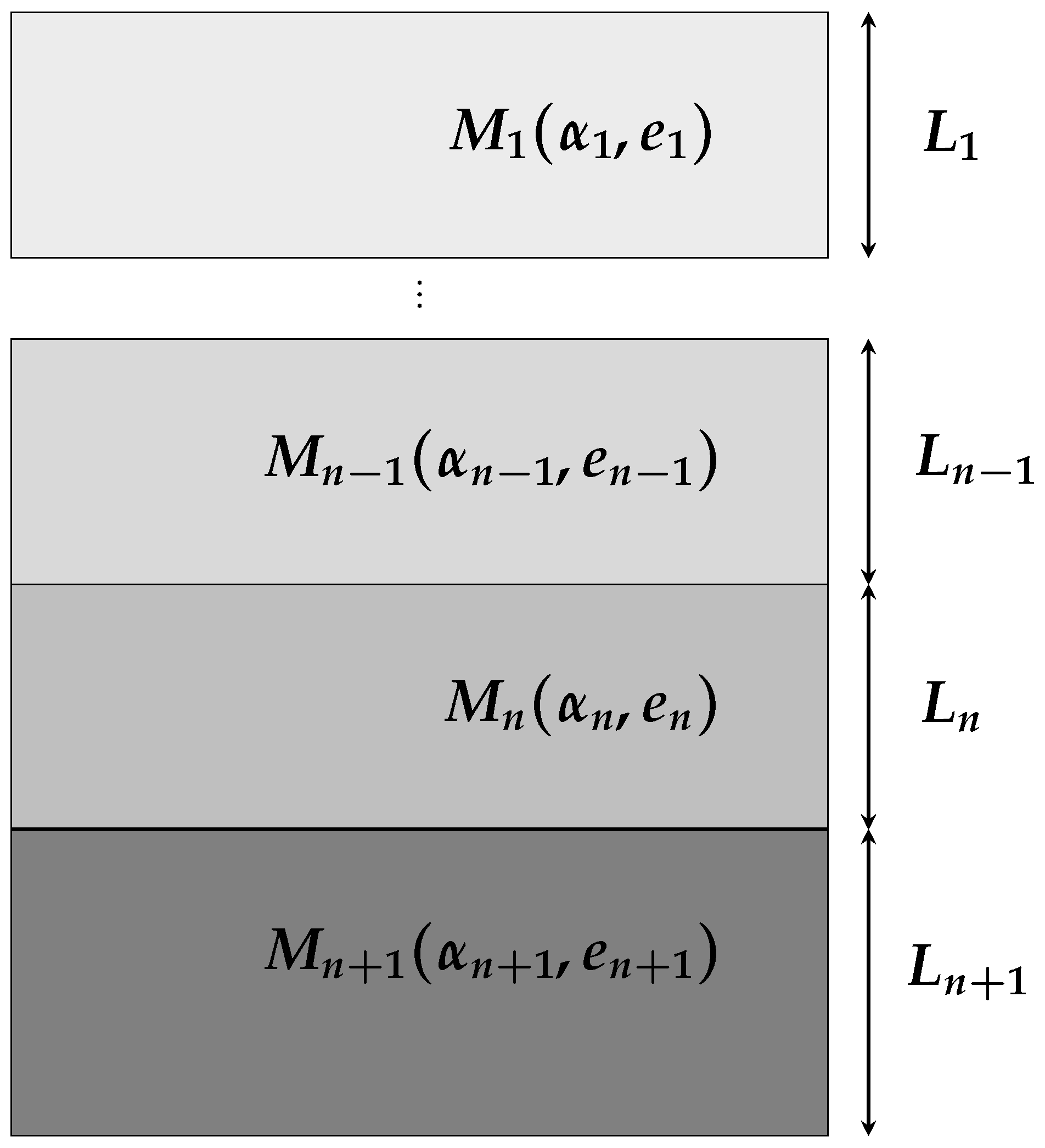
In this article, general multi-layered coating systems of total layers, where coating layers of different materials are applied on top of each other on a substrate material are investigated, see Figure 1. For , denotes the thickness of the associated layer. The thermal properties of each material are characterized by the thermal diffusivity and the thermal effusivity .
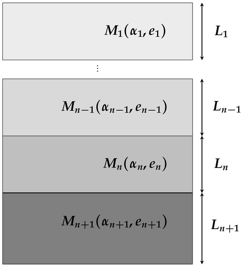
Figure 1.
System of n coating layer materials , …, on a substrate material .
The determination of
using a method of nondestructive testing is of great interest in the manufacturing process and quality control of such systems. In the following, a few application examples for a varying number of coating layers are listed.
:
- The manufacturing process of electrode coatings of Lithium-ion batteries, where a Lithium cobalt oxide coating of 50 to μm is applied to a thin (μm) aluminum substrate. Inaccurate coating thicknesses lead to performance issues of the battery or higher production costs.
- The application of non-electrolytic zinc-aluminum flakes to protect metallic surfaces by increasing their corrosion resistance.
:
- Production of plastic housings of laptops or smartphones. For example, the substrate might be some rigid ABS plastic of 1 to 2 mm, the first thin coating layer (the so-called basecoat) might be some polyurethane (μm) that acts like a thermal insulator against the increasing heat of the electronics, and the second coating layer (the so-called topcoat of μm) might be some UV hardened resin acting like a visually appealing surface finish.
:
- In the automotive and aviation industries [1,2], where metallic or CFRP substrates are coated with different paints, e.g., a primer, basecoat, topcoat, and clearcoat. Here again, each layer fulfills its own function, and it is, therefore, necessary to control the individual layer thicknesses.
There are some issues to be taken into account when choosing an appropriate measuring process (cf. [3]). Eddy current or inductive-based measurement methods only work on metallic substrates, and X-ray or beta backscattering methods only work with certain metal groups and also require compliance with strict occupational health and safety, radiation protection, and disposal measures. Furthermore, ultrasonic and capacitive methods need contact with the test specimen and are therefore not suitable for measuring wet coatings (e.g., for the automotive paint process line) or uncured powder coatings. A very promising method, which is contact-free and uses harmless and non-invasive electromagnetic radiation, is presented by the terahertz technology; see [2]. Unfortunately, the usage of highly sensitive devices is needed, such as a femtosecond laser, which is often prohibitively expensive for medium-sized companies.
In this article, it is suggested that photothermal methods, such as infrared thermography, are especially suited for the measurement of multi-layered coating systems. Such methods are contact-free and have manageable costs. A typical setting is presented in Figure 2, where the components and the operating principle are as follows:
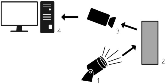
Figure 2.
Measurement principle of infrared thermography.
- 1
- Optical excitation sources, such as lamps or lasers (cf. [4], [Chapter 4]), irradiate an object under investigation with optical (i.e., visible) light. Its task is to produce the photothermal effect, i.e.,
- 2
- The test object absorbs the optical energy (light) and converts it into thermal energy (heat). Heat transfer inside the test object occurs, which is dependent on the characteristics of the object geometry, its material composition, and thermal properties.
- 3
- The thermal response of the test object is recorded by a measuring device, such as an infrared camera.
- 4
- Finally, a computer processes and evaluates the data to provide certain properties (or even defects) of the considered test object.
It should be mentioned that the photothermal method requires only two conditions:
- The investigated coatings must be susceptible to optical radiation in a certain wavelength regime, i.e., for near-infrared, visible, or UV light.
- There must be a thermal contrast between two adjacent layers. Otherwise, a transparent interface would be created without significant reflection.
There are mainly two classical optical excitation types in thermographic processes, i.e., the lock-in thermography and pulsed thermography; see e.g., [5,6,7]. The latter method analyses the transient response and propagation of heat pulses in the test object. A prominent processing technique in pulsed thermography is the TSR (Thermographic Signal Reconstruction) method, where the logarithmic time derivatives of the signal are examined, cf. [8,9,10]. However, pulsed thermography has been used mainly for one-layered coating systems so far or simple defects. Since the intensity of the pulse decreases strongly in almost all materials, high energies are sometimes necessary to cause significant heating of the test object. In addition, this method is error-prone in case of surface irregularities, and the infrared camera would need a very high frame rate in order to detect reflections from multiple-layer interfaces in multi-layered coating systems.
Lock-in thermography, whose principle the article is based on, means that the surface of the test object is periodically modulated using a planar sinusoidal waveform with a fixed frequency. Since the generated thermal wave has the same frequency as the excitation, especially the phase angle (or phase difference) as a result of thermal wave interference carries a lot of information. The goal is to determine from phase angle data for different modulation frequencies measured by an infrared camera. Since thermal waves show the same behavior as optical waves in the visible spectral range, thermal reflection, and transmission coefficients can be derived; see e.g., [11,12]. Hence, thickness estimation from phase angle measurements represents an inverse problem; see (cf. [13,14,15,16]) for corresponding literature.
The overview and contributions of this article are summarized as follows:
- Section 2 discusses the basics of thermal wave generation and thermal wave interference in the well-established one-layered and two-layered coating cases. Subsequently, these principles are used in order to obtain a new thermal wave interference formula in multi-layered coating systems with coating layers on a thermally thick substrate.
- Section 3 defines the forward operator for a known number of coating layers, which maps to the phase angle data with m being the number of used modulation frequencies. The inverse operator is then defined, which approximates an inversion of by solving a nonlinear least squares problem. Finally, since are often partially or even completely unknown, a concept is additionally presented, which utilizes the generated data of multiple samples in a clever way, where the unknown thermal properties can also be determined and used to calibrate a model for the layer thickness determination.
- Section 4 concludes with numerical experiments that demonstrate the performance of the developed layer thickness determination procedure.
2. Mathematical Setup
To understand the physical process of thermal wave interference for the general case of multi-layered coating systems, it is necessary to take a closer look at known models for semi-infinite media and for the cases with and coatings. The mathematical notations and formulations in the next subsections can be found in [4,17,18,19].
2.1. Basics of Thermal Wave Generation
Thermal waves can be mathematically characterized as solutions of the heat diffusion equation. The heat source at the surface represents the boundary conditions, influences the surface temperature distribution, and determines the generation of waves. The most common type of excitation is a periodic, planar energy input with high-performance laser beams of a single specific excitation frequency, i.e., lock-in excitation.
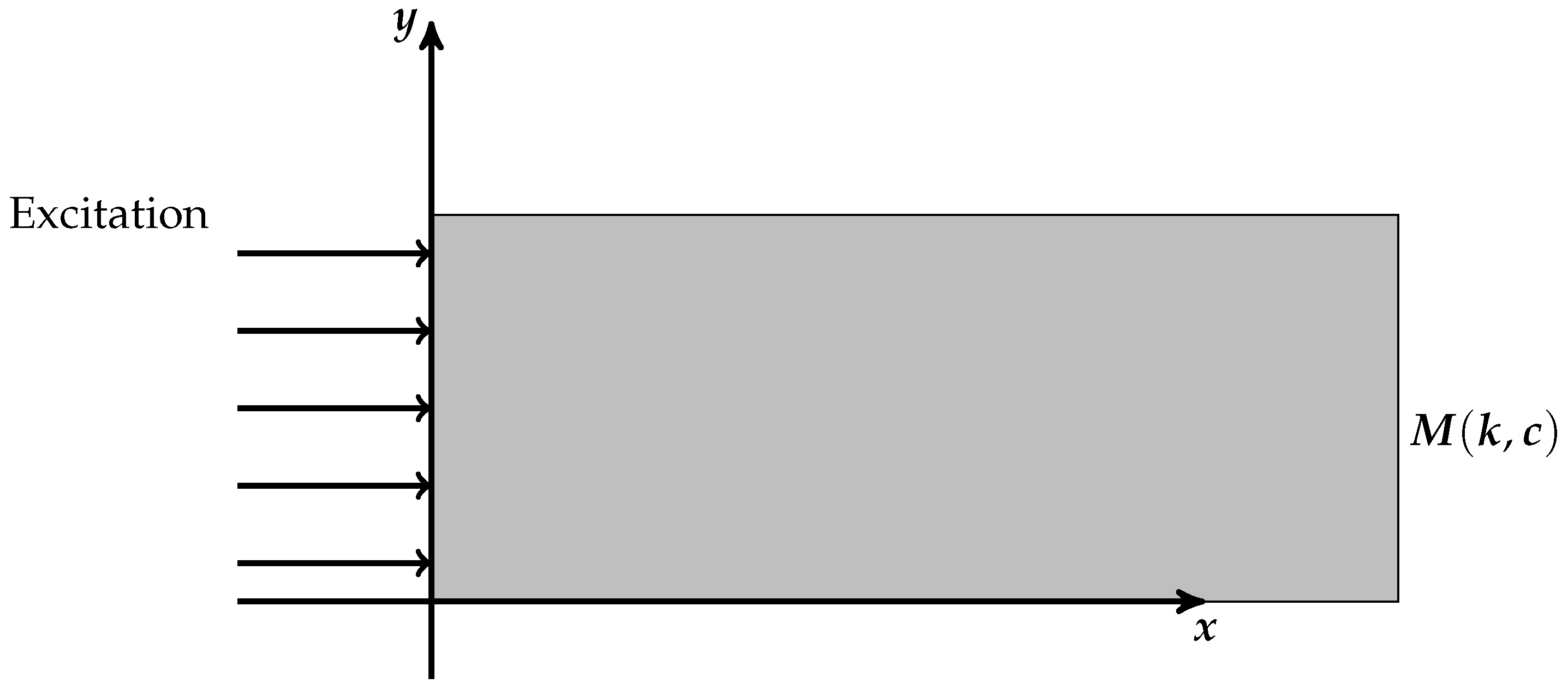
For the sake of simplicity, an isotropic homogeneous semi-infinite medium M (that means an infinite extension of the medium in x-direction) is considered, which is illustrated in Figure 3.
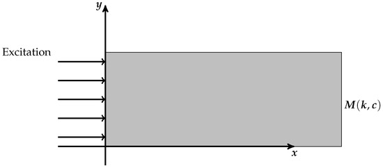
Figure 3.
Thermal wave generation and propagation in a semi-infinite medium.
Here, k denotes the thermal conductivity, and c denotes the volumetric heat capacity of the material M. The thermal diffusivity can then be calculated using and the thermal effusivity by .
It is assumed that the heated surface occupies the -plane at . To obtain the temperature distribution at the surface of the medium, the Fourier equation must be solved,
First, the boundary conditions need to be specified. The medium’s surface is excited with a plane harmonic; thus, temporal heating of modulation frequency for some frequency f and source intensity . This leads to an excitation of the form
yielding the generation of thermal waves inside the medium.
Since the periodic thermal energy is subject to conduction into the solid, by using the appropriate rate equation, the boundary condition on the surface is given as
Here, dc means the Direct Current and ac the Alternating Current. The dc component will not be relevant in later applications and can be neglected. Applying a time-harmonic approach then yields
Plugging this in Equation (1), one ends up with
Taking into account that must be finite for , one receives the solution of the boundary value problem (1) and (2) as
Using a multiplication with and further simplifications, one obtains a more significant expression given as
where
is the so-called thermal diffusion length.
Hence, thermal waves are significantly dampened, where controls the penetration depth into the material. For small thermal diffusivity , the thermal waves do only slightly propagate into the interior of the material. In contrast, by decreasing the modulation frequency , a deeper penetration of the thermal waves into the material is obtained. This phenomenon is very useful in the photothermal measurement of layer thicknesses.
Furthermore, note that there occurs a progressive phase shift using
between the temperature at the surface and a point x located at the propagating thermal wave in the material. Thus, at the surface , an expressive phase difference of between the excitation source and the resulting surface temperature can be observed.
2.2. Transmission and Reflection
If the irradiated object is not a semi-infinite medium but a composition of at least two materials M and (with thermal effusivities e and , respectively), the thermal wave travels through M first towards and, if the planar thermal wave propagation direction is perpendicular to its interface, the thermal reflection and transmission coefficients are
with
being the thermal refraction index, which characterizes the thermal contrast between the two media. If there is no thermal contrast, i.e., if , it follows that . In this case, there would be no significant reflection from this interface and, therefore, no contribution to thermal wave interference effects influencing the surface temperature. Thus, for a determination of coating layer thicknesses it is crucial to guarantee that the materials are distinguishable, i.e., .
In the following, whenever indices are added to the reflection or transmission coefficient, this is assigned to the interface between the materials and . The direction of these coefficients has to be understood downwards, cf. Figure 1. For the upward direction, a prime is added to the notation. For example,
The only exception regarding the direction is for and , where the top surface of first layer material is exposed to air , i.e.,
The reader is referred to [4] for a more detailed derivation of the expressions above.
2.3. Basics of Thermal Wave Interference
In this subsection, the basics of thermal wave interference using an investigation of the cases of and coatings are discussed. Here, mathematical formulas are well established, cf. [4,18,19]. For the convenience of the reader, the results are summarized before the insights are extended to multi-layered coating systems.
2.3.1. One-Layered Coatings on a Substrate
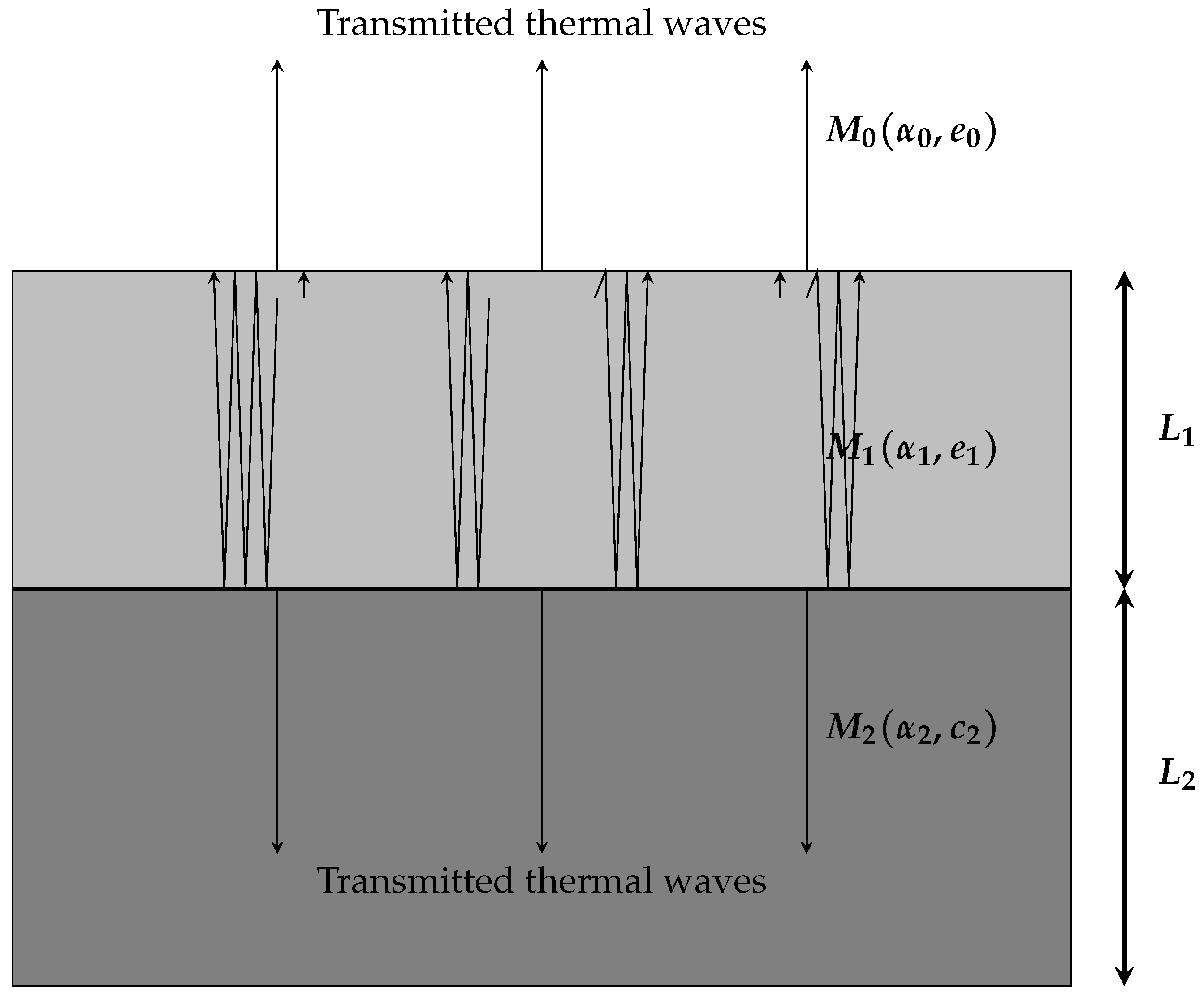
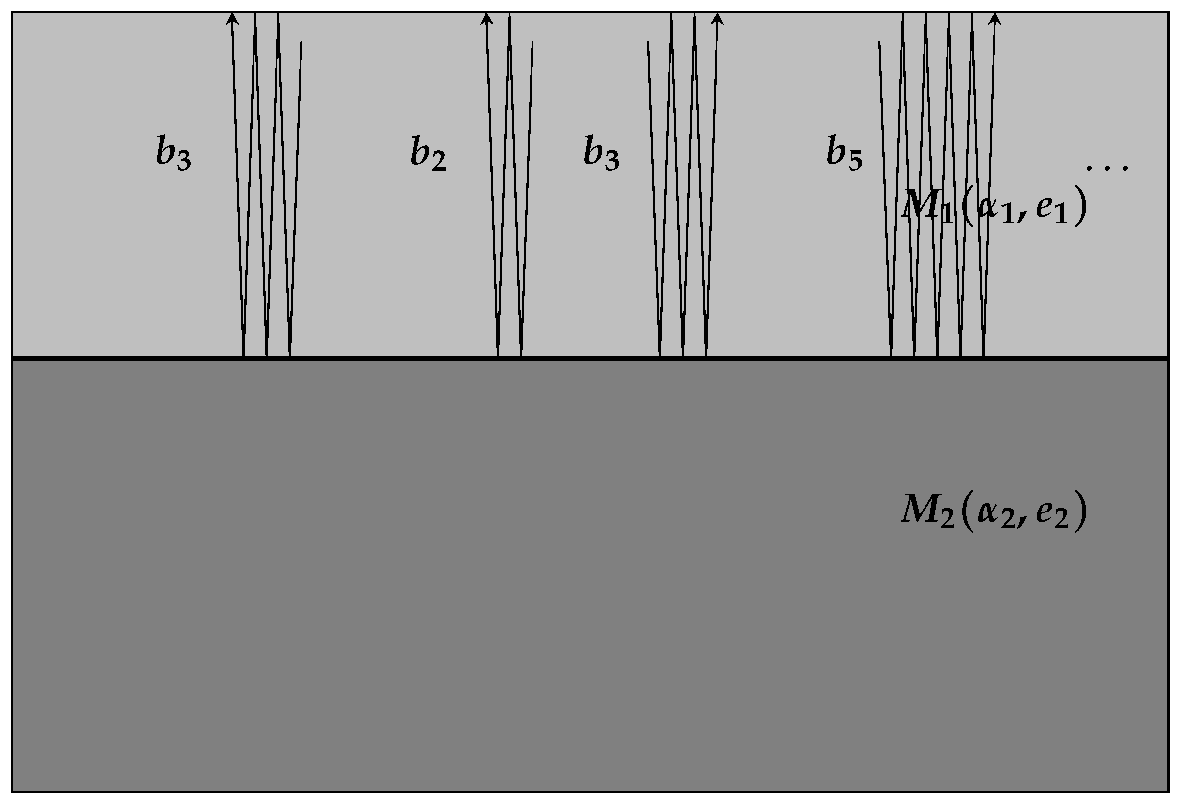
Consider the following system of two layers consisting of media and , as illustrated in Figure 4.

Figure 4.
Thermal wave interference in one coating layer on a thermally thick substrate material.
Assume that both media and have homogeneous thermophysical properties and that has thickness and has thickness . Furthermore, assume that is thermally thick. That means that is significantly larger than the thermal diffusion length . This assumption is not unusual, as the substrate is often much thicker than the applied coating. This guarantees that the transmitted thermal waves into the substrate do not have an effect on the surface temperature because they can be neglected due to the large attenuation. Moreover, assume that the whole system is exposed to air (denoted by ). Suppose that the surface is illuminated by a plane, normal and periodic heating.
The single wave trains that are generated near the surface propagate towards the interface between the two media and back towards the surface of . When meeting any interfaces, the waves are partially reflected and transmitted. Thermal wave interference effects occur, meaning that the surface temperature at is a sum of all thermal wave trains. In general, when a thermal wave has traveled a distance the amplitude will be damped by , where is the complex wave number. Hence, for the first reflection order wave train in material , the thermal wave has a propagation path of length leading to an attenuation by . The following figures include sketches of thermal wave trains and give the impression that there is a lateral diffusion in the material itself. This, however, does not hold true since only one-dimensional propagation is present. The sketches serve only for graphic visualization.
Note that no bulk absorption of the absorbed radiation is considered in this article. This means that the photothermal effect provides surface heating only, i.e., thermal waves originate exclusively near . The presented references distinguish between the following two cases:
- (1)
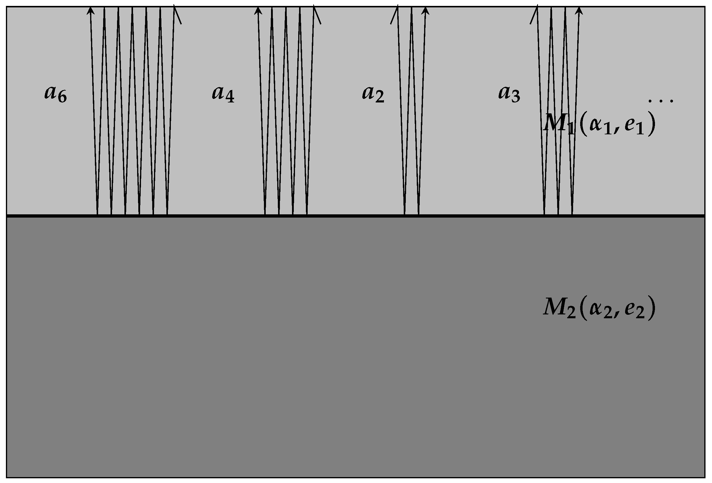
- Waves that are first reflected from the interface between and , see Figure 5:
 Figure 5. Waves that are reflected first at the interface between and .Let denote the nth reflection order wave and the reflection coefficient at the interface between and ( and , respectively). Furthermore, let denote the transmission coefficients at the interface between and in the upward (downward) direction. Since the single wave trains are reflected at the interface “infinitely” often, one obtains the following series corresponding to the surface temperature:where the geometric series formula is used, since holds true.
 - (2)
- For waves that are first reflected from the interface between and , see Figure 6, let denote the nth reflection order wave. Analogous to the first case, one obtains the following expression corresponding to the surface temperature fraction:where the geometric series formula is used, since holds true.
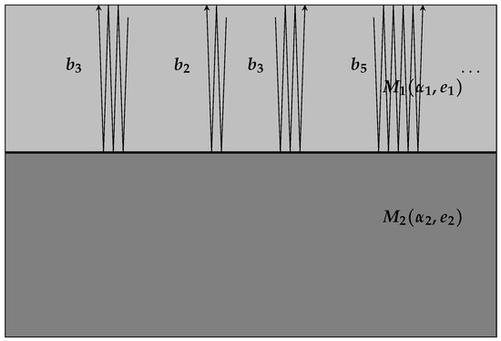 Figure 6. Waves that are reflected first at the interface between and .
By summing up both series, one obtains the thermal wave interference expression at the surface:
This provides the following expression for the time-dependent temperature at the surface:
Note that the phase shift in this formula, given by , is excluded and has the meaning of normalizing the temperature by subtracting an “infinitely” thick layer, cf. Equation (6).
The wave vector is complex and so is the temperature amplitude. It can be split into its real and imaginary parts providing an expression in polar coordinates. To this end, one sets
and calculate
and
Define . Then the amplitude is obtained using
as well as the phase angle
which provides an expression for the complex temperature amplitude at the surface in polar coordinates, i.e.,
The advantage is that the amplitude, as well as the phase, are measurable real valued expressions.
2.3.2. Two-Layered Coatings on a Substrate
Next, consider the following system of three layers, –, having thicknesses –, where is assumed to be thermally thick.
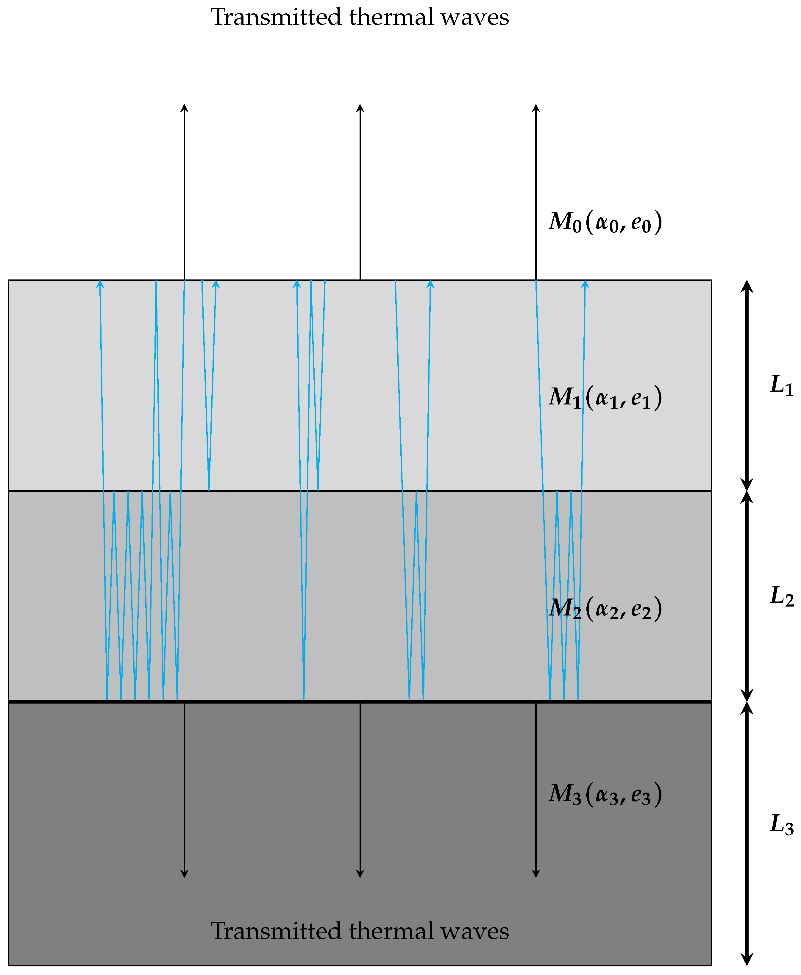
Obviously, adding a second coating layer increases the complexity in which thermal wave trains can possibly propagate in the system, see, for example, the blue arrows in Figure 7. The first interface for the case was a coating-to-substrate interface, while for the first interface is a coating-to-coating interface. Transmitted thermal waves can no longer be ignored, because the second layer is not thermally thick anymore, i.e., the reflections still contribute to the surface temperature significantly, although they have a longer propagation path. A very elegant way of summarizing all possible wave trains is done by replacing a complex-valued effective reflection coefficient for the real-valued reflection coefficient from Equation (11), cf. [4,19].
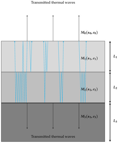
Figure 7.
System of two layers of coatings – and one layer of substrate .
Again, by introducing a new layer, the reflection process expands after passing the interface between and and appear at a lower level, too. Thus, interference effects occur in the new layer with material as well. This implies that the reflection coefficient is not sufficient to describe the whole process anymore, so it is necessary to change the expression in analogously to the derivation in Equation (9) as
Here, ( denotes the transmission coefficients in a downward (upward) direction at the – interface. Using (), one denotes the reflection coefficients at the same interface, where the thermal wave train stays in (). Analogously, is the reflection coefficient for thermal waves in that stay in .
Therefore, because of , the geometric series formula can be used again, since . Note that
which effectively represents the case again, if the second coating layer would be infinitely thick (or at least thermally thick).
The quantity is called the effective reflection coefficient. Since the thermal interference processes are the same in the first layer as discussed before, one ends up with the following surface temperature for :
Once again, this expression provides a term for the amplitude,
as well as for the phase angle,
yielding
2.4. Generalization to Multi-Layered Coating Systems
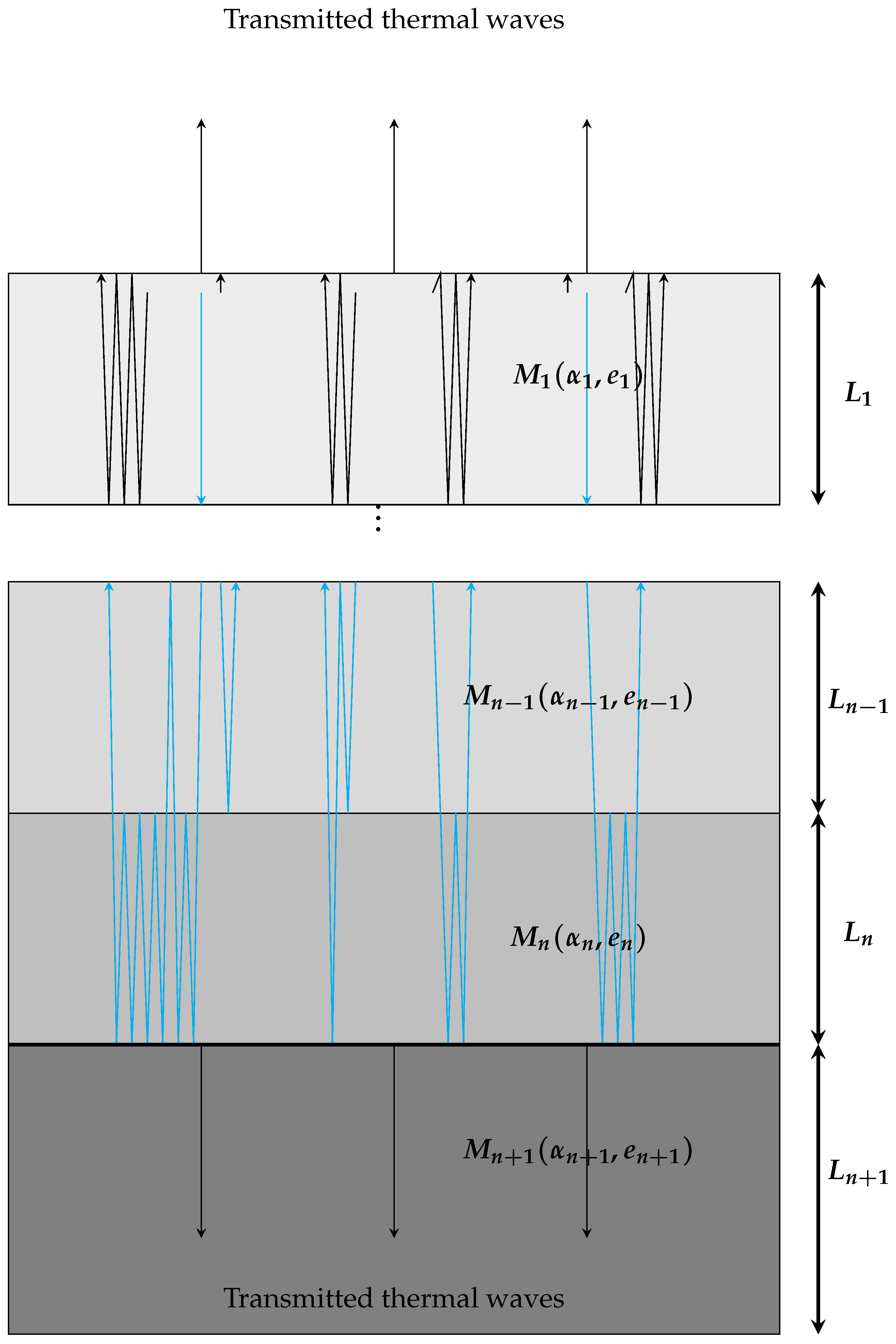
The subject of the investigations is to make use of the insights outlined before and generalize Formula (17) for a multi-layered coating system; see Figure 8. Consider the following system consisting of layers of coatings with material – having thicknesses – on a thermally thick substrate material .
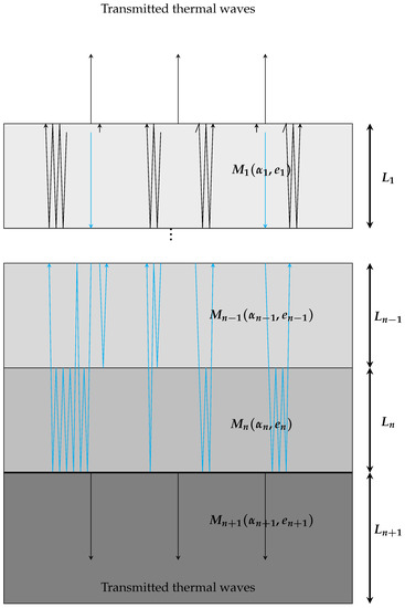
Figure 8.
System of n layers of coating materials – and one layer of substrate .
For , the idea was to look at the last reflection coefficient from the case and, since a new layer is added, replace it by some effective reflection coefficient including all potential wave trains that are apparent in the new system. This principle can be extended further, which leads to nested effective reflection coefficients, i.e., one defines recursively with
Although the generalized formula for the surface temperature of multi-layered coating systems looks as for , i.e.,
the effective reflection coefficient now contains all the significant information about the coating system, such as the layer thicknesses , the thermal diffusivities , and the thermal effusivities . Note that and are not of any interest because the substrate is thermally thick, but is needed for the calculation of .
3. Layer Thickness Determination
After a mathematical model for the physical process of thermal wave interference has been deduced, the inverse problem of computing from phase angle measurements can be formulated. Furthermore, the situation of unknown thermal properties will be addressed, and a solution will be presented in a separate subsection.
3.1. Forward and Inverse Operator
As discussed in the preceding section, the thermal properties needed for the calculation of the surface temperature of a coating system with n layers can be summarized with the vector
For and frequencies , define the forward operator
which maps to vector of phase angles , cf. Equation (21). Note, that in (23) the dependencies on and were dropped since these are kept fixed, but it is sometimes practicable to use the extended notations,
For the determination of , assume that an infrared camera measures the temperature response of such a system for every frequency. After some post-processing of the signals (cf. [5,20,21]), the phase angle data
are given.
The inverse operator is defined by
which maps the phase angle data to the layer thickness vector by minimizing a nonlinear least-squares functional. Here, denotes the Euclidean norm.
3.2. Unknown Thermal Properties and Issues with All-at-Once Optimization
The approach (Equation (25)) seems unusable for real-world applications as the thermal properties of every coating layer must be known. For example, in the automotive industry, paint mixtures are changed occasionally, and it does not make sense to perform a complex thermal analysis each time. In general, what is available for the calibration of any nondestructive testing device are different samples of a fixed multi-layered coating setup with varying but known coating layer thicknesses. These are typically measured either in a destructive (e.g., cross-sectional images under the microscope, etc.) or non-destructive (e.g., laser triangulation, X-ray, etc.) way. Whether this coating layer thickness information of every layer in every sample is gathered before or after the frequency scans and phase angle data collection with an infrared camera depends on the method in use. However, it is worth noting that this process only needs to be performed once for each coating system setup.
In the following, a concept to identify the needed thermal properties in order to determine of such coating systems is presented. As a first idea, one can replace the functional from Equation (25) with
which represents an all-at-once approach, i.e., all unknown parameters are determined simultaneously. Unfortunately, this approach shows the following ambiguity issue: For every , terms of the form
imply
i.e.,
since the thermal contrast between the layers and, thus, the reflection coefficients are identical. Hence, it is necessary to decouple the determination of and . This can be done by utilizing the sample data in a clever way.
Assume that samples (n coating layers with different but known for ) are available for the calibration process. Modulation of every sample surface by the frequencies leads to a total amount of phase angle values, i.e.,
For , the entire batch of sample data is divided in two sets
and proceeded with the following steps.
STEP 1: Determine thermal properties from , i.e.,
STEP 2: Feed the thermal properties from STEP 1 into the objective functional and determine the coating layer thicknesses of sample j by
for . Evaluate the results for by calculating the error
If the error (28) is sufficiently small, depending on the accuracy requirements of the manufacturing process itself, the coating system setup is calibrated and tested successfully. If a higher accuracy is needed, further samples need to be processed, or needs to be adjusted. Of course, the usage of more frequencies also improves the quality of the data.
4. Numerical Experiments
In this section, the implementation of (25) is presented and numerical experiments are discussed. For the minimization process
the function lsqnonlin from the MATLAB Optimization Toolbox is used, which provides a solver for nonlinear least-square problems by utilizing a reflective trust-region algorithm. The function requires an initial value . Optionally, also a lower and upper bound () can be specified, where the order relation is to be understood component-wise. The reader is referred to the lsqnonlin documentation website for further details.
The following numerical simulations investigate the one-layered, the two-layered, and the three-layered system, i.e., coating layers of different paints on top of a thermally thick aluminum substrate material modeling the painting line in the automotive industry. The thermophysical properties of the included materials are known and given by Table 1:

Table 1.
Thermal properties used in the experiments.
These values are needed in order to be able to determine the thermal diffusion lengths of every material and the effective reflection coefficients on the interfaces.
In each experiment, the substrate layer is the same, and the coating layers are chosen in ascending order. Therefore, the case represents the paint layer 1 on the aluminum substrate, whereas for , the paint layer 2 is between the paint layer 1 and the substrate. For , also paint layer 3 is between paint layer 2 and the substrate. For reasons of simplicity, each coating layer possesses the same thickness of m (), i.e.,
In order to vary the penetration depth of the thermal waves, the excitation frequency f (and therefore the angular frequency ) can be adjusted. In this context, it is worth noting that it is recommended to use sufficiently small frequencies leading to deeper penetration of all materials in every setting. In order to test whether it is possible to reconstruct the exact layer thicknesses from the phase angle data, the data need to be generated by forward calculation (23), i.e., for given frequencies one computes
For every experiment, 20 initial values are chosen in the interval of with equidistant spacing. The results in the following tables show the reconstructed as well as the average relative error of the phase angles
where is the relative error of the phase angle associated with the j-th frequency. The relative error is calculated by the absolute value of the difference of the phase angle of the exact thickness and the calculated thickness, divided by the phase angle of the exact thickness.
4.1. Experiment 1,
Let m be the exact thickness of the first layer (Paint layer 1, cf. Table 1) on the thermally thick aluminum substrate. The experimental parameters are as follows:
- (1.1)
- Set 20 initial values with equidistant spacing. The given angular modulation frequencies are
- (1.1.1)
- Hz,
- (1.1.2)
- Hz,
- (1.1.3)
- Hz,
- (1.1.4)
- Hz and Hz.

Table 2.
Results for case (1.1.1).

Table 3.
Results for case (1.1.2).

Table 4.
Results for case (1.1.3).

Table 5.
Results for case (1.1.4).
4.2. Experiment 2,
Consider the system of three total layers (Paint Layer 1 on Paint Layer 2 on Aluminum Substrate) with specified thermophysical properties according to Table 1. Let m be the exact thicknesses of the coating layers. The experimental parameters are as follows:
- (2.1)
- Set 20 initial values with equidistant spacing. The given angular modulation frequencies are
- (2.1.1)
- Hz,
- (2.1.2)
- Hz, Hz,
- (2.1.3)
- Hz, Hz, Hz.

Table 6.
Results for case (2.1.1).

Table 7.
Results for case (2.1.2).

Table 8.
Results for case (2.1.3).
4.3. Experiment 3,
Consider the system of four total layers (Paint Layer 1 on Paint Layer 2 on Paint Layer 3 on Aluminum Substrate) with specified thermophysical properties according to Table 1. Let m be the exact thicknesses of the coating layers. The experimental parameters are as follows:
- (3.1)
- Set 20 initial values with equidistant spacing. The given angular modulation frequencies are
- (3.1.1)
- Hz, Hz, Hz,
- (3.1.2)
- Hz, Hz, Hz, Hz.

Table 9.
Results for case (3.1.1).

Table 10.
Results for case (3.1.2).
4.4. Observations
Regardless of the number of chosen layers, similar observations in each experiment can be deduced. Accurate results are achieved for if the number of excitation frequencies is at least as large as the number of searched layer thicknesses. Choosing only a single frequency (Table 2, Table 3 and Table 4) for the one-layered case (Experiment 1, ) shows that frequency adaption is needed such that the data carry sufficient information for the solver to reconstruct the thickness for every initial value. Here, Table 4 represents the overall best results for the lowest frequency. Adding a second frequency (Table 5) does not seem to improve the results and may appear unnecessary, but since it enriches the data, it stabilizes the minimization process in such a way that the frequency adaption can be omitted. Choosing only a single frequency (Table 6) for the two-layered case (Experiment 2, ) is insufficient, although it can generate good results when the initial value is close to the exact solution . Again, adding more frequencies to the process for Experiment 2, one is able to reconstruct for the majority of the initial values.
Obviously, the average relative error is not an appropriate indicator for the approximation accuracy of ; see e.g., Table 2 for the initial value , where the relative average error is actually negligible, but the calculated thickness shows a relative error of approximately 25 percent. This is a typical behavior of nonlinear inverse problems, suggesting that minimizing the objective functional (Equation (25)), even with exact data, can lead to inexact solutions. Only in a few cases is the algorithm unable to find an appropriate minimizer
at all, such that the residual is ; see e.g., Table 9 for the intial value , but the average relative error is approximately 90 percent. Here, the algorithm stops in a local minimum since the initial value has not been chosen appropriately. Comparing results for multiple initial values is therefore crucial in order to evaluate the calculated . With increasing n, the structure of the objective functional gets more complex. This often leads to strings of initial values getting trapped in undesired local minima, which complicates the evaluation of the results. For example, the results of the last six initial values in Table 9 give the impression that has to be accepted as a solution, whereas the exact solution is only represented four times in the middle section of the same table. Adding a fourth frequency (Table 10) resolves this ambiguity and leads to the exact result.
5. Conclusions
In this article, multi-layered coating systems have been investigated consisting of coating layers on a thermally thick substrate, which are periodically illuminated using a planar, sinusoidal waveform with a fixed frequency. This illumination generates a thermal wave of the same frequency, which is reflected and transmitted at the interfaces. The surface temperature, which can be measured by an infrared camera, is a result of the superposition of all thermal wave trains propagating through the system. A new model was developed that describes the physical process of 1D thermal wave interference in such setups. This model describes the dependencies of the coating layer thicknesses, the frequency used, and the thermal properties of the layers to the measured phase angle data. Given measured phase angles as data, the inverse operator was defined in order to compute the coating layer thicknesses. The problem of unknown thermal properties was discussed, and a concept to determine these in advance was proposed. Finally, numerical experiments for the determination of the coating layer thicknesses were performed, which prove the performance of the method and suggest that the amount of applied frequencies has to be sufficiently large. Additionally, it has been demonstrated that the comparison of results of multiple initial values is important for the evaluation process.
Author Contributions
Conceptualization, D.R. and T.S.; methodology, D.R.; software, D.R.; validation, D.R.; formal analysis, D.R.; investigation, D.R.; writing—original draft preparation, D.R.; writing—review and editing, T.S.; visualization, D.R.; supervision, T.S.; project administration, T.S.; funding acquisition, T.S. All authors have read and agreed to the published version of the manuscript.
Funding
This research was funded by the European Fund for Regional Development from the Operational Program EFRE Saarland 2014–2020 with the objective Investments in Growth and Employment.

Institutional Review Board Statement
Not applicable.
Informed Consent Statement
Not applicable.
Data Availability Statement
Not applicable.
Acknowledgments
We are indebted to Stefan Böttger and Thomas Karwoth from AIM Systems GmbH for fruitful discussions and cooperation within the project. We would also like to thank Eileen Oberringer for her assistance with the numerical results. We acknowledge support by the Deutsche Forschungsgemeinschaft (DFG, German Research Foundation) and Saarland University within the “Open Access Publication Funding” program.
Conflicts of Interest
The authors declare no conflict of interest.
Symbols and Abbreviations
The following abbreviations are used in this manuscript:
| A0 | Thermal wave amplitude at point of generation |
| Thermal diffusivity | |
| c | Volumetric heat capacity |
| e | Thermal effusivity |
| f | Modulation frequency |
| Phase angle | |
| Effective reflection coefficient | |
| k | Thermal conductivity |
| L | Layer thickness |
| M | Material |
| Heat source intensity | |
| R | Reflection coefficient |
| Complex wave number | |
| T | Transmission coefficient |
| Complex temperature amplitude | |
| Periodic temperature, dependent on position x and time t | |
| Thermal diffusion length | |
| Angular Modulation frequency |
References
- Ellrich, F.; Bauer, M.; Schreiner, N.; Keil, A.; Pfeiffer, T.; Klier, J.; Weber, S.; Jonuscheit, J.; Friederich, F.; Molter, D. Terahertz quality inspection for automotive and aviation industries. J. Infrared Millim. Terahertz Waves 2020, 41, 470–489. [Google Scholar] [CrossRef]
- Krimi, S.; Klier, J.; Jonuscheit, J.; von Freymann, G.; Urbansky, R.; Beigang, R. Highly accurate thickness measurement of multi-layered automotive paints using terahertz technology. Appl. Phys. Lett. 2016, 109, 021105. [Google Scholar] [CrossRef]
- Gholizadeh, S. A review of non-destructive testing methods of composite materials. Procedia Struct. Integr. 2016, 1, 50–57. [Google Scholar] [CrossRef]
- Almond, D.; Patel, P. Photothermal Science and Techniques; Chapman & Hall: London, UK, 1996. [Google Scholar]
- Wu, D.; Busse, G. Lock-in thermography for nondestructive evaluation of materials. Rev. Générale De Therm. 1998, 37, 693–703. [Google Scholar] [CrossRef]
- Breitenstein, O.; Langenkamp, M. Lock-in Thermography; Basics and Use for Functional Diagnostics of Electronics Components; Springer: Cham, Switzerland, 2003. [Google Scholar]
- Chatterjee, K.; Tuli, S.; Pickering, S.G.; Almond, D.P. A comparison of the pulsed, lock-in and frequency modulated thermography nondestructive evaluation techniques. NDT E Int. 2011, 44, 655–667. [Google Scholar] [CrossRef]
- Shepard, S.M.; Lhota, J.R.; Rubadeux, B.A.; Wang, D.; Ahmed, T. Reconstruction and enhancement of active thermographic image sequences. Opt. Eng. 2003, 42, 1337–1342. [Google Scholar] [CrossRef]
- Shepard, S.M.; Beemer, M.F. Advances in thermographic signal reconstruction. In Proceedings of the Thermosense: Thermal Infrared Applications XXXVII, SPIE, Baltimore, MD, USA, 20–24 April 2015; Volume 9485, pp. 204–210. [Google Scholar]
- Balageas, D.L.; Roche, J.M.; Leroy, F.H.; Liu, W.M.; Gorbach, A.M. The thermographic signal reconstruction method: A powerful tool for the enhancement of transient thermographic images. Biocybern. Biomed. Eng. 2015, 35, 1–9. [Google Scholar] [CrossRef] [PubMed]
- Greiner, W. Klassische Elektrodynamik; Harri Deutsch Verlag: Thun, Switzerland, 2008; Volume 55606. [Google Scholar]
- Macke, W. Thermodynamik und Statistik: Ein Lehrbuch der Theoretischen Physik; Akademische Verlagsgesellschaft Geest & Portig K.-G.: Leipzig, Germany, 1962; Volume 5. [Google Scholar]
- Louis, A.K. Inverse and Ill-Posed Problems; Springer: Berlin/Heidelberg, Germany, 2013. [Google Scholar]
- Schuster, T.; Kaltenbacher, B.; Hofmann, B.; Kazimierski, K.S. Regularization Methods in Banach Spaces; Walter de Gruyter: Berlin, Germany, 2012; Volume 10. [Google Scholar]
- Rothermel, D.; Schuster, T.; Schorr, R.; Peglow, M. Determination of the Temperature-Dependent Thermal Material Properties in the Cooling Process of Steel Plates. Math. Probl. Eng. 2021, 2021, 6653388. [Google Scholar] [CrossRef]
- Rothermel, D.; Schuster, T. Solving an inverse heat convection problem with an implicit forward operator by using a projected quasi-Newton method. Inverse Probl. 2021, 37, 045014. [Google Scholar] [CrossRef]
- Carslaw, H.S.; Jaeger, J.C. Conduction of Heat in Solids; Oxford University Press: Oxford, UK, 1947. [Google Scholar]
- Palmer, J.M.; Grant, B.G. The Art of Radiometry; SPIE Press: Bellingham, MA, USA, 2010. [Google Scholar]
- Lepoutre, F.; Fournier, D.; Boccara, A. Nondestructive control of weldings using the mirage detection. J. Appl. Phys. 1985, 57, 1009–1015. [Google Scholar] [CrossRef]
- Busse, G.; Wu, D.; Karpen, W. Thermal wave imaging with phase sensitive modulated thermography. J. Appl. Phys. 1992, 71, 3962. [Google Scholar] [CrossRef]
- Dillenz, A.; Zweschper, T.; Riegert, G.; Busse, G. Progress in Phase Angle Thermography; AIP Publishing: New York, NY, USA, 2003. [Google Scholar]
Disclaimer/Publisher’s Note: The statements, opinions and data contained in all publications are solely those of the individual author(s) and contributor(s) and not of MDPI and/or the editor(s). MDPI and/or the editor(s) disclaim responsibility for any injury to people or property resulting from any ideas, methods, instructions or products referred to in the content. |
© 2023 by the authors. Licensee MDPI, Basel, Switzerland. This article is an open access article distributed under the terms and conditions of the Creative Commons Attribution (CC BY) license (https://creativecommons.org/licenses/by/4.0/).

