Recognition and Pose Estimation Method for Stacked Sheet Metal Parts

Abstract

To address issues such as detection failure and the difficulty in locating gripping points caused by the stacked placement of irregular parts in the automated sheet metal production process, a highly robust method for the recognition and pose estimation of parts is proposed. First, a decoding framework for parts of a two-dimensional code is established. The morphological closed operation and topology of contours are used to locate the two-dimensional code, and the type of the part is decoded according to the structure of the two-dimensional code extracted by the projection method. Second, the recognition model of the occluded part type is constructed. The edge information of parts is extracted. The contour convex hull is used to split the part contours, and the similarity of segmented contours is calculated based on the Fourier transform. Finally, the occluded parts are located. The corner points of the metal parts are extracted by the adjacency factor of the differential chain code sequence and the contour radius of curvature. The transformation matrix between the part and the standard template is calculated using similar contour segments and contour corner points. A stereo vision system is built to detect and localize the irregular sheet metal parts for experiments, including detection and information extraction experiments of the two-dimensional laser-generated code and detection and positioning experiments of parts under different occlusion rates. The experimental results show that the decoding framework can accurately decode the two-dimensional code made by a laser under low-contrast conditions, the average recognition rate can reach 93% at multiple occlusion rates, the geometric feature extraction algorithm is more accurate than common algorithms and no pseudo-corner points, the localization error is less than 0.8 mm, and the pose angle error is less than 0.6°. The methods proposed in this paper have high accuracy and robustness.

1. Introduction

Sheet metal parts are widely utilized in aviation, ships, automobiles, home appliances, etc. The variety of products is complex and in great demand, but the lack of flexibility in operations, such as sorting and assembly in the manufacturing process, results in high labor intensity and low efficiency [1,2]. Currently, sheet metal is only automatically produced for products with similar structures and no occlusions. The identification and localization technology for parts that are arbitrarily shaped and positioned under partial occlusion conditions still has numerous flaws, and there are still problems such as type detection failure and low localization accuracy. Therefore, research has been conducted to address these issues.

In industrial production, a quick response code is frequently implemented to achieve the identification and management of sheet metal parts, CNC (computer numerical control) tools, and other metal parts [3]. It can also address the traceability and flow of sheet metal parts. Although the decoding mechanism for QR (quick response) codes is rather advanced, in real-world applications, issues such as inconsistent lighting and randomly placed workpieces can easily result in location failure. Therefore, improving the decoding rate depends greatly on the accurate location of the QR code [4]. At present, machine learning and deep learning methods are commonly used to locate the target [5]. Machine learning and deep learning methods are often applied in the field of automated manufacturing with certain stability [6,7]. These methods are commonly used for coarse localization of 2D (two-dimensional) codes, but they are deficient in correcting target offset angles or extracting structural information. The traditional QR code localization method determines the location information with the pixel scale feature of three location detection graphs 1:1:3:1:1 [8], which is vulnerable to pixel quality and feature extraction algorithms, with poor stability and a high misclassification rate. On this premise, some scholars have achieved advancements. Gao Fei located the minimum outer rectangle of the outer graph contour and refined the skeleton structure to achieve precise 2D code positioning, and Gao Fei located the minimum outer rectangles of the position detection patterns’ contours and refined the skeleton structure to achieve precise 2D code positioning, even though the encoding structure is prone to causing abnormal minimum outer rectangle positioning [9]. Feng Wei achieved QR code correction and localization by extracting the recognition location detection graph’s center coordinates for indirect leveling [10]. Tian Zhen used the Hough transform to extract the 2D code edge lines, calculated the offset angle, and positioned it [11]. These two methods were less robust with complex contours. However, the randomly stacked parts are partially occluded, and the method of recognizing parts based on weak textures, such as QR codes, may not work.

In vision applications, such as face recognition, industrial production, and intelligent driving, detecting occluded targets is a difficult problem. Missing features brought on by the reciprocal occlusion of targets make recognition and localization more difficult [12,13]. As an important and stable feature for the recognition of occluded target types, contours are the object of intensive research by domestic and foreign scholars. Song Jianhui compared the occluded contour fragment with the rest of the spatial contour position to achieve good recognition in the case of large-area occlusions, but the method is only applicable to cases where there are discrete contour fragments of the target [14]. Krolupper F used curvature information to segment contours and measured similarity based on approximating polygons, whereas the algorithm segmentation results are less accurate and more susceptible to occlusions [15]. Huang Weiguo used the spatial contour location relationship to construct the chord angle feature descriptors of contour sampling points and calculated the matching similarity by an integral graph algorithm, but the method is more complex and is not suitable for industrial production [16]. Shi Siqi and Rui Lu described contour features using a shape context, but the algorithm is weak in noise immunity [17,18]. For localization of parts under local occlusion, Wang Shuyu obtained features such as hole contours and fitted circle center coordinates for weakly textured workpieces by geometric constraints, but the algorithm suffers from false detection in the case of uneven illumination [19]. Yu Zhenjun created a template using the part corner point feature set, established a geometric hash table, and achieved target matching according to the voting mechanism, but the algorithm efficiency is affected by the number of segmentation points [20]. Zheng JingYi combined the graphical cutting method with the shape prior model to locate occluded workpieces, whose algorithm accuracy depends on the model segmentation results and applies to regular parts [21].

To solve problems such as the detection failure and positioning difficulties of sheet metal parts when multiple types of targets, occluded targets, and irregular targets exist, in this paper, a part recognition and pose estimation method with an automatic vision system for sheet metal is used as the research object. First, the framework for partial surface 2D laser-generated code identification and decoding is established. According to the encoding arrangement rule, the morphological closed operation is used for rough positioning, and the deviation is corrected by the contour topology of the position detection patterns. The encoding information is extracted according to the projection method, and the part type can be easily interpreted. Second, the type recognition model of occluded parts is constructed. Using the boundary line segment method, the boundary is effectively segmented with the concept of the convex hull, and the normalized Fourier descriptor of the segmented contour is calculated. The Euclidean distance is used to measure the similarity and identify the type of occluded parts. Finally, the workpiece geometric features are extracted based on the adjacency factor of the first-order contour difference in the Freeman chain code sequence and the contour curvature, and the position pose results are obtained by combining the a priori contour matching information to locate the occluded part.

2. Identification of Sheet Metal Parts

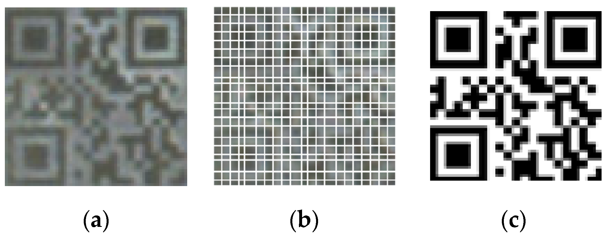
2.1. Positioning and Structure Extraction of Two-Dimensional Laser-Generated Code

The two-dimensional laser-generated code contains the sheet metal part’s identity information. However, the placement of the part affects the image of the two-dimensional laser-generated code, and the contrast varies from placement to placement. As shown in the low-contrast image in Figure 1, the high-band edges of the two-dimensional code structure are prone to weakening and blurring, resulting in positioning failure and unclear information extraction. As a result, to improve the accuracy of two-dimensional code decoding, this paper proposes a two-dimensional code localization and structure extraction method. First, the morphological closed operation is used to coarsely locate the two-dimensional code region according to the law of two-dimensional code arrangement. Second, the contour topology of the position detection pattern is used for fine localization. Finally, the structure of the QR code is extracted by segmenting the encoding module using the projection method.

The morphological closure operation expands and then contracts the image, which effectively excludes the QR code’s internal voids. This operation effectively reduces the complexity of the features and achieves encoding structure homogeneity. The image is then binarized. The four-linked two-pass method labels the set of all connected domains. Some noise points are removed because they are too small in area and lack descriptive shape power. The two-dimensional code position is initially determined based on the height-to-width ratio of the smallest outer rectangle of the connected domains.

The position detection patterns serve as the foundation for precise positioning of the two-dimensional code, and three position detection patterns can be used to calculate the position and offset angle of the two-dimensional code. The patterns have an obvious multilayer nested contour topology. One pattern’s contours can be identified as the external or internal boundary of the hole. These can be represented, like in Figure 2, by the labels $cX$ and $hX$, where $X$ stands for a number, $c$ for “contour”, and $h$ for “hole” or inner contour. A contour tree can be constructed using this label. In Figure 2, for instance, c0 represents the contour of the root node, h00 represents the child node of c0, and h00 also contains the new child node c000. The contour tree of the pattern can be used to determine the topology of the contour. Because this feature has a high level of anti-interference, the topology, shape, and statistical moments of the contours can be used to locate the position detection patterns. The specific judgment conditions are as follows:

$$\{\begin{array}{l}{W}_{c0}/H_{c0}=W_{h00}/H_{h00}=W_{c000}/H_{h000}\approx 1\\ L_{c000}:L_{h00}:L_{c0}\approx 3:4:5\\ m_{c0}\left(x,y\right)\approx m_{h00}\left(x,y\right)\approx m_{c000}\left(x,y\right)\end{array}$$

(1)

As shown in Equation (1), $W$ and $H$ represent the length and width of the contour’s minimum external rectangle, L represents the contour’s length, and m represents the contour’s center. By using Equation (1), it is possible to locate three position detection patterns.

Figure 3 illustrates the location of the smallest external rectangle and the center coordinates $m\left(x,y\right)$ of the three location detection graphs of the QR code used in Equation (1). In Figure 3, $m_i$ is the position detection pattern’s center coordinates, and $p_i$ is the QR code’s four vertices. The center point coordinates $m_1$ of position 1 and $m_2$ of position 2 are used to calculate the equation of the line $l_{m_1{m}_2}:ax+by+c=0$. The projection point O of the center point coordinates $m_0$ of position 0 on $l_{m_1{m}_2}$ establishes the center of the QR code, which is

$$\{\begin{array}{l}{x}_o=\frac{b\left(-b{x}_{m_0}+a{y}_{m_0}\right)+ac}{-a^2-b^2}\\ y_o=\frac{bc-a\left(-b{x}_{m_0}+a{y}_{m_0}\right)}{-a^2-b^2}\end{array}$$

(2)

The center point $m_0$ of position 0 is linked to the QR code’s center point O. The distance $s$ between the position detection pattern’s center coordinates $m_i$ and the boundary is calculated using the QR code version information $v$. The $l_{om0}$ line is extended to obtain the position 0 boundary point $p_0$. Calculating the symmetry point $p_3$ of point $p_0$ about line $l_{m1m2}$ yields the boundary point of position 3. The specific formulas are as follows:

$$s=\frac{\frac{1}{2}\left(\left|m_0{m}_1\right|+\left|m_0{m}_2\right|\right)\left(v-1\right)}{2\left(v-7\right)}$$

(3)

$$\{\begin{array}{l}{x}_{p_3}=x_{p_0}-\frac{2a\left(ab{x}_{p_0}+b{y}_{p_0}+c\right)}{a^2+b^2}\\ y_{p_3}=y_{p_0}-\frac{2b\left(a{x}_{p_0}+b{y}_{p_0}+c\right)}{a^2+b^2}\end{array}$$

(4)

Using boundary distance $s$, boundary points $p_1$ and $p_2$ are calculated by extending the straight line $l_{m_1{m}_2}$ using the boundary length $s$. The encoding area is then precisely located using the four calculated boundary points. The QR code’s angular offset is corrected by using the angle $\alpha$, which is calculated from the angle between line $l_{m_1{m}_2}$ and the normal.

The projection method is utilized to grid the code area. The projection method involves accumulating the pixel values of the contour image $P\left(x,y\right)$ of the 2D code in both the horizontal and vertical directions. Then, the inverse difference is performed on the set of pixel projections in the horizontal and vertical directions. The distribution of the wave peaks of the contour projection waveform map can be obtained by the projection method, and each wave peak represents the regional peak of the accumulated contour and the alternate boundary of the encoding structure. The set of peaks in both directions can be used to vertically and horizontally segment the encoding region. The projection method equation is as follows:

$$\{\begin{array}{l}l\left(x\right)=\nabla {\displaystyle {\sum }_{y}P\left(x,y\right)}\\ l\left(y\right)=\nabla {\displaystyle {\sum }_{x}P\left(x,y\right)}\end{array}$$

(5)

The split single grid represents a module that is either black or white. The average grayness of each module is counted to obtain an average grayness distribution matrix G of a two-dimensional code as follows:

$$\mathit{G}={\left[\begin{array}{cccc}{g}_{11}& g_{12}& \cdots & g_{1v}\\ g_{21}& g_{22}& \cdots & g_{2v}\\ ⋮& ⋮& \ddots & ⋮\\ g_{v1}& g_{v2}& \cdots & g_{vv}\end{array}\right]}_{v\times v}$$

(6)

In Equation (6), $g_{ii}$ denotes the mean grayscale value of a single module. The matrix size is related to the encoding version $v$. Using the maximum interclass variance method on the mean grayscale matrix, the encoding characteristics can be obtained.

2.2. Recognition Algorithm of Occluded Sheet Metal Parts

The boundary contour of an irregular sheet metal part contains one or more depressions, as shown in Figure 4. Therefore, it is possible to segment the boundary contours using the convex hull and convex defects.

Contour matching requires accurate contour detection algorithms with a high signal-to-noise ratio. As the optimal edge detection method, the Canny algorithm can accurately extract the actual edges of the target. The convex hull algorithm is then used to determine the minimum convex hull $S$ of the part’s outer contour, as shown below:

$$S=\left\{{\displaystyle \sum _{j=1}^n{t}_j{c}_j}|c_j\in C,{\displaystyle \sum _{j=1}^n{t}_j=1,t_j\in \left[0,1\right]}\right\}$$

(7)

In Equation (7), $c_j$ represents the part’s contour points. Figure 5a depicts the convex hull structure of the component derived using Equation (7). Each convex defect in the illustration consists of the inner contour of the depression and the line connecting the convex defect’s endpoints. Multiple extremely minor convex defects are caused by the contour curve’s noise. Many erroneous segmentation points will be generated if two endpoints of each convex defect are used as the contour segmentation points. According to the size of the convex defects and the length of the inner contour of the depression, the noise in the curve can be eliminated. The set of segmented segments obtained by this method is $Z=\left\{z_i\right\}\left(i=1,2,3,\dots ,K\right)$, and the optimized segmentation results and convex hull are shown in Figure 5b.

Recognition of the segmented contour segments requires the description of features. Normalized Fourier descriptors of contours exhibit invariance to translation, rotation, and scaling. Consequently, the Fourier descriptors of the contour segments can be retrieved and utilized as prominent features for segmented target recognition. Assume that a single contour segment consists of $N$ points. The two-dimensional coordinates of the $N$ contour points are converted to the plural as follows:

$$z\left(n\right)=x\left(n\right)+y\left(n\right),n=0,1,2,\cdots N-1$$

(8)

In Equation (8), the x-axis of the coordinates is the real axis of the plural, and the y-axis of the coordinates is the imaginary axis of the plural. The descriptors $z\left(u\right)$ of the contour obtained using the discrete-time Fourier transform can be expressed as

$$z\left(u\right)=\frac{1}{N}{\displaystyle \sum _{u=0}^{N-1}z\left(n\right)}{e}^{-\frac{j2\pi un}{N}},u=0,1,2,\cdots ,N-1$$

(9)

The plural sequence can be reconstructed by the inverse Fourier transform, as shown in the following equation:

$$z\left(n\right)={\displaystyle \sum _{n=0}^{N-1}z\left(u\right)}{e}^{\frac{j2\pi un}{N}},n=0,1,2,\cdots ,N-1$$

(10)

The high-frequency components of the Fourier transform reflect the target’s specific characteristics, while the low-frequency components describe the target’s overall shape. To determine the description of a small number of descriptors for the entire contour, the L-term Fourier descriptors are extracted for contour reconstruction. For contour reconstruction, 40%, 20%, 10%, 5%, and 2.5% of the Fourier descriptors from 568 contour points are retrieved accordingly. Figure 6 displays the contour coordinate points that were reconstructed using 224, 112, 56, 28, and 14 descriptors. Figure 6 demonstrates that as the number of descriptors increases, the contours’ finer details become increasingly apparent. The image with 14 descriptors lacks the features of the contours. The image with 28 descriptors can describe the contour better, and the total amount of information is reduced to 5% that of the original. Normalizing the Fourier descriptors results in the descriptors $d\left(u\right)=\frac{\Vert z\left(u\right)\Vert }{\Vert z\left(1\right)\Vert }$.

Mutual orthogonality exists between the frequency components of the Fourier transform. Therefore, the Euclidean distance can be used to measure the difference between different contour segments and to find similar contour segments. The following is the metric function:

$$Distance=\sqrt{{\displaystyle \sum _{u=2}^L\Vert d_I\left(u\right)-d_J\left(u\right)}{\Vert }^2}$$

(11)

In Equation (11), $I$ and $J$ represent different contour fragments.

3. Position Estimation of the Occluded Parts

3.1. Freeman’s Chain Code

The vectorized chain code sequence of the contour curve is established by the eight-direction Freeman chain code. The coding scheme is shown in Figure 7. Taking the target pixel $pi$ as the center, the directivity of the next pixel $p_{i+1}$ on the contour is determined along the eight-pixel directions $\left\{b_i,i=0,1,2,\dots ,7\right\}$ of the neighborhood. $i$ is the direction amplitude, and the whole contour curve is traversed in turn to obtain the chain code sequence with shape information.

3.2. Smoothing Contours

There are random mutation points caused by noise in contour detection. In Figure 8, the four typical mutation instances are depicted. These mutations increase the complexity of the contour description and lead to errors in the geometric feature extraction process. Therefore, the contour and chain code are restored by the first-order differential information of the chain code.

The first-order difference process records the number of changes in the adjacent two chain code elements in the eight counterclockwise direction, which can be expressed as follows:

$$a_i^{\prime }=\left(a_i-a_{i-1}\right)\mathrm{mod}M$$

(12)

In Equation (12), $a_i$ denotes the chain code element, mod denotes the modulo operation, and $M$ denotes the number of chain code directions. The chain code and the chain code differential sequence are analyzed. When $a_i^{\prime }=2,6$, $a_{i-1}=a_i\ne a_{i+1}$, and $a_{i-2}=a_{i+1}=0,2,4,6$, and then $a_{i-1}$ and $a_i$ are assigned. The mutation point is found by traversing the contour along the counterclockwise direction, and the contour information and chain code sequence are smoothed.

3.3. Geometric Feature Extraction Method

The first-order differential chain code sequence reflects the number of changes in the chain code’s pointing values. $a_i^{\prime }\ne 0$ indicates that the contour’s point may not be on the same line as the next contour’s point and may be a corner of the contour. Thus, the contour corner points’ potential locations can be originally determined using the differential chain code.

As illustrated in Figure 9, some pseudo-corner points arise when the contour is described by the Freeman chain code. Therefore, it is necessary to incorporate the contour’s curvature information to evaluate the corner points. Curve pieces are taken from the $w$ contour points that are close to the front and back of the corner points. Curvature estimation is achieved by calculating the radius of curvature of the curve segments, and the curvature estimation method is depicted in Figure 9. Endpoints A and C of the curve are connected, and Helen’s formula is used to calculate the distance $h$ between the suspected corner point B and line segment AC.

$$h=\frac{1}{2a}\sqrt{p\left(p-a\right)\left(p-b\right)\left(p-c\right)}$$

(13)

In Equation (13), $p=\frac{1}{2}\left(a+b+c\right)$, and $a$, $b$, and $c$ are the side lengths of triangle ABC. The distance $Q$ and the arch height $h$ can be used to obtain the radius of curvature $R$ of the circle. Using the adjacency factors of the Freeman chain code sequence and differential chain code sequence, contour pointing analysis is performed to address the problem in that the radius of curvature between adjacent suspicious points varies with a small magnitude, resulting in an inability to precisely locate corner points such as point E in Figure 9. Observing the pointing values of the neighboring chain codes $a_{i+n}$ and $a_{i-n}$ before and after to exclude suspicious approximation points, the point is not a contour’s corner point if the adjacent chain codes are consistent or if there is periodic repetition. The remaining corner points and their curvature radii are stored for part location.

3.4. Calculation of the Transformation Matrix

Based on the Freeman chain code and the contour curvature, it is possible to find the feature points of the template part and the measured component. As shown in Figure 10, the Fourier descriptor can be used to identify the contour segments of the occluded parts. Then, as matching conditions, the radius of curvature of feature points on the identified contour segments and the distance between feature point pairs are utilized to extract at least three pairs of matching points. The matching point pairs are utilized to calculate the poses of the occluded part and obtain the initial values of registration between the template contour and the measured contour. The transformation matrix for the pose of the part is shown in Equation (14):

$$\left[\begin{array}{l}X\\ Y\end{array}\right]=\left[\begin{array}{cc}{a}_{11}& a_{12}\\ a_{21}& a_{22}\end{array}\right]\left[\begin{array}{l}x\\ y\end{array}\right]+\left[\begin{array}{l}\Delta x\\ \Delta y\end{array}\right]$$

(14)

In Equation (14), $\left(X,Y\right)$ denotes the feature point set of the contour after the pose transformation. The cumulative distance error between $\left(X,Y\right)$ and the set of measured contour feature points is calculated as follows:

$$E_s={\displaystyle \sum _{i=1}^K\sqrt{{\left(x_i^{\prime }-X\right)}^2+{\left(y_i^{\prime }-Y\right)}^2}},i=1,2,3$$

(15)

All geometric feature points on the part contour are traversed in the counterclockwise direction. As the distance judgment threshold between matched point pairs, the initial value of cumulative error is utilized. Matched point pairs with low curvature similarity or a curvature similarity greater than the error threshold are eliminated, and matched point pairs that satisfy the geometric feature restrictions are removed. RANSAC (random sample consensus) is utilized to fit the pose transformation matrix of the matched point pairs.

4. Experimental Results and Analysis

4.1. Vision System Construction

The experimental system consists of a data acquisition and data processing device. The data are collected using a binocular camera, transmitted using a GigE network port connection, and then analyzed and processed using a computer. Based on the information in the data, the parts are identified and located.

The data acquisition section consists of two Hikvision monocular industrial CMOS (complementary metal–oxide–semiconductor) cameras. The cameras’ model is MV-CA013-20GC from Hikvision in Hangzhou, China. The resolution of cameras is 1280 × 1024 pixels. Both camera lenses have a focal length of 12 mm, and the field of view is approximately 410 mm × 280 mm at a working distance of 800 mm. The cameras are attached by a bracket plate and fixed on a tripod, as shown in Figure 11. Multiple sets of images of 10 mm × 10 mm glass calibration plates were taken for camera calibration to obtain the internal and external reference matrices of the camera and the reprojection error of the calibration. The calibration results are shown in Figure 12, and the average reprojection error is 0.15 pixels. The input image size of the calibration experiment is 1280 × 1024 pixels, so the average reprojection error is 0.0092% of the diagonal of the image, which shows that the calibration results are reliable.

The calibration experiment can obtain the rotation matrix R and translation matrix T centered on the left camera, as follows:

$$\mathit{R}=\left[\begin{array}{ccc}0.9982& 0.0083& -0.0584\\ -0.0080& 1.0000& 0.0047\\ 0.0584& -0.0043& 0.9983\end{array}\right]$$

(16)

$$\mathit{T}=\left[\begin{array}{ccc}-58.9648& 0.4425& 2.3870\end{array}\right]$$

(17)

4.2. Part Identification Experiment

4.2.1. Two-Dimensional Code Positioning and Structure Extraction Experiments

For QR code decoding experiments, the camera shoots some randomly placed sheet metal parts. This subsection runs tests on low-contrast OR code images to ensure the stability of the QR code decoding framework. Figure 13 depicts the images produced by each stage of the QR code localization algorithm, from coarse to fine localization. As seen, this method is capable of effectively localizing the low-contrast encoding region.

Figure 14 depicts the waveforms of the QR code contour’s horizontal and vertical projections. Backward differencing the projection values in the horizontal and vertical directions yields the projection peak, which is used to grid segment the target area. Figure 15a depicts the QR code grid segmentation result. As shown in Figure 15b, the structure of the code is obtained based on the distribution matrix of the gray mean of the segmented QR code, and the structure is clearer when compared with the original QR code image. The Zbar algorithm can quickly determine the part’s type.

4.2.2. Identification Experiment of Occluded Parts

Images of the stacked sheet metal parts are acquired for experiments. The edge information of the part is detected using the Canny operator, as shown in Figure 16. In contour detection, it is impossible to effectively segment the overlapping areas of stacked parts. Therefore, multiple part contours of stacked parts are identified. As illustrated in Figure 17b, the part contours are retrieved for segmentation, and segment descriptors are generated. Utilizing a template-matching database of normalized Fourier descriptors, similar contour segments of the parts are identified. Figure 17 displays the identification outcomes (c).

Different degrees of occlusion occur in randomly stacked and placed parts. To validate the robustness of the occlusion target recognition approach, one thousand photos of parts are gathered to generate detection data. The data collected contain photos of sections with occlusion rates of 10%, 20%, 30%, 40%, and 50% at a ratio of 1:1:1:1:1. Experiments were conducted on the data set, and the results are shown in Figure 18.

Figure 18 shows the target recognition accuracies of algorithms with occlusion rates ranging from 10% to 50%. The algorithm shows in the case of local occlusion: the higher the occlusion rate, the fewer the contour features and the lower the accuracy rate. The recognition algorithm in this paper has an accuracy of higher than 90% at occlusion rates of less than 40% and an average detection accuracy of 93% at multiple occlusion rates. The method has a good recognition effect.

4.3. Location Experiments of Occluded Parts

The type information of the part is obtained by the identification algorithm. Then, the same type of template can be used to effectively estimate the pose matrix and complete the localization. To verify the efficacy and accuracy of the positioning method, the occluded parts are rotated at various angles and then placed randomly to record their respective position information. The pose transition matrix of the occluded parts in 200 images is calculated to obtain the localization accuracy of the algorithm.

In the experiments, the localization algorithm obtains the geometric feature points for template matching based on the adjacency factor and contour curvature features of the Freeman chain code. To verify the accuracy of the feature extraction algorithm, it is compared with the Harris, Shi-Tomasi, and CSS (curvature scale space) operators. The various algorithms are analyzed by detecting the contour corner points of the part template, and the detection results of several algorithms are displayed in Figure 19.

According to Figure 19, the number of missing corner points in the detection results of the Harris operator and Shi-Tomasi operator is small, and there are some pseudo-corner points. More corner points are missed in the detection results of the CSS operator. In contrast, the improved algorithm in this paper can obtain the corner points of irregular parts and effectively capture the feature points of some parts with weak contour changes, and there are no pseudo-corner points with high accuracy.

The geometric features of the inspected part are obtained by the algorithm. Figure 20 shows the feature point coordinates, curvature circle, and curvature radius of the part. The contour matched point pairs of the template and the inspected part are extracted to obtain the part’s positional transformation matrix, as in the following equations:

$${\mathit{M}}_1=\left[\begin{array}{ccc}0.9106& 0.4031& -226.5685\\ -0.4031& 0.9106& 187.6361\end{array}\right]$$

(18)

$${\mathit{M}}_2=\left[\begin{array}{ccc}0.9960& -0.0047& 5.8746\\ 0.0047& 0.9960& -3.2181\end{array}\right]$$

(19)

Due to the part’s irregular shape, its center of gravity is chosen as the grasping point. The part’s center of gravity is calculated to obtain the position error. The pose angle error is obtained by comparing the workpiece’s pose angle with the actual rotation angle. Error analysis is conducted on 200 test data results, and the results are displayed in

Table 1. Mean and root mean square errors in the positioning of occluded parts.

Positioning Errors	Mean Errors	Root Mean Square Errors
x direction/mm	0.65	0.74
y direction/mm	−0.21	0.58
position angle/(°)	0.47	0.54

.

Table 1 shows the mean error and root mean square error of the localization algorithm. According to the root mean square error, the positioning error of the stacked parts is less than 0.8 mm, and the pose angle error is less than 0.6°. The localization algorithm can precisely determine the pose transformation matrix of occluded parts to localize occluded targets.

To further demonstrate the efficacy of the method, the localization results for irregular parts at various angles or occlusion rates are provided. Figure 21a,b display the results of the algorithm for estimating the parts’ position at 20% and 40% occlusion rates. The algorithm can find the same parts as the template, even when they are occluded by nonidentical shaped parts, as in Figure 21c. The algorithm is also applicable when multiple parts are stacked, as in Figure 21d, and can be used to locate parts that are occluded in multiple parts.

5. Conclusions

The aim of this study is to effectively solve problems such as detection failure or difficulty in locating the grasping points for irregular sheet metal parts when random stacking occurs. In this research, a part identification and pose estimation approach is proposed. The part information is obtained by establishing a two-dimensional code decoding framework for parts. To enhance the reliability of part recognition, a contour template matching model is built for occluded parts. Location estimation results are obtained by combining a priori contour information with geometric features. A stereo vision system is constructed to perform recognition and localization experiments on the occluded parts. The experimental results show that the algorithm can accurately locate and extract two-dimensional laser-generated code features and improve the decoding rate; the recognition algorithm has an accuracy of higher than 90% at occlusion rates of less than 40%, and the average recognition rate can reach 93%; the localization algorithm can effectively capture geometric features; the localization error is less than 0.8 mm; and the pose angle error is less than 0.6°. The accuracy and stability of the method are both high.

In this paper, the accuracy of data collected by a 1.3-megapixel industrial camera is low, and the accuracy will be higher using a higher-resolution data collection device. One type of long irregular part is tested in this paper; if more irregular parts have been experimented with, the stability of the algorithm will be better verified. The algorithm in this paper is mainly for thin parts, and the algorithm for parts’ detection with certain thicknesses needs to be improved in the future.

References

1. Liu, S.; Xia, Y.; Shi, Z.; Yu, H.; Li, Z.; Lin, J. Deep Learning in Sheet Metal Bending with a Novel Theory-Guided Deep Neural Network. IEEE-CAA J. Autom. 2021, 8, 565–581. [Google Scholar] [CrossRef]
2. Murena, E.; Mpofu, K.; Ncube, A.T.; Makinde, O.; Trimble, J.A.; Wang, X.V. Development and performance evaluation of a web-based feature extraction and recognition system for sheet metal bending process planning operations. Int. J. Comput. Integr. Manuf. 2021, 34, 6. [Google Scholar] [CrossRef]
3. Ventura, C.; Aroca, R.; Antonialli, A.; Abrão, A.; Rubio, J.C.; Câmara, M. Towards Part Lifetime Traceability Using Machined Quick Response Codes. Procedia Technol. 2016, 26, 89–96. [Google Scholar] [CrossRef] [Green Version]
4. Okazaki, S.; Navarro, A.; Mukherji, P.; Plangger, K. The curious versus the overwhelmed: Factors influencing QR codes scan intention. J. Bus. Res. 2019, 99, 498–506. [Google Scholar] [CrossRef] [Green Version]
5. Yuan, B.; Li, Y.; Jiang, F.; Xu, X.; Guo, Y.; Zhao, J.; Zhang, D.; Guo, J.; Shen, X. MU R-CNN: A Two-Dimensional Code Instance Segmentation Network Based on Deep Learning. Future Internet 2019, 11, 197. [Google Scholar] [CrossRef] [Green Version]
6. Elsheikh, A.H. Applications of machine learning in friction stir welding: Prediction of joint properties, real-time control and tool failure diagnosis. Eng. Appl. Artif. Intell. 2023, 121, 105961. [Google Scholar] [CrossRef]
7. Elsheikh, A.H.; Elaziz, M.A.; Vendan, A. Modeling ultrasonic welding of polymers using an optimized artificial intelligence model using a gradient-based optimizer. Weld. World 2021, 66, 27–44. [Google Scholar] [CrossRef]
8. Wang, W.; He, W.; Lei, L. 2-D Bar Code Data Extraction on Metal Parts. J. Comput.-Aided Des. Comput. Graph. 2012, 24, 612–619. [Google Scholar]
9. Gao, F.; Ling, Q.; Ge, Y. Location Method of Laser QR Code Based on Position Discrimination. J. Comput.-Aided Des. Comput. Graph. 2017, 29, 1060–1067. [Google Scholar]
10. Feng, W.; Fang, C. Stable localization algorithm of QR code based on method of least squares. App. Res. Comp. 2018, 35, 957–960. [Google Scholar]
11. Tian, Z.; Wang, M.; Liu, Z. Research and design of QR code recognition system based on Intelligent display line. Mfg Automn 2022, 44, 159–163. [Google Scholar]
12. Hu, Y.; Liu, F.; Wei, Z. Vehicle Tracking of Information Fusion for Millimeter-wave Radar and Vision Sensor. China Mech. Eng. 2021, 32, 2181–2188. [Google Scholar]
13. Xu, J.; Liu, N.; Li, D. A Grasping Poses Detection Algorithm for Industrial Workpieces Based on Grasping Cluster and Collision Voxels. Robot 2022, 44, 153–166. [Google Scholar]
14. Song, J.; Song, X.; Yu, Y. Occlusion targets recognition using contour fragments spatial relationship. J. Huazhong Univ. Sci. Technol. 2019, 47, 79–83. [Google Scholar]
15. Krolupper, F.; Flusser, J. Polygonal shape description for recognition of partially occluded objects. Pattern Recognit. Lett. 2007, 28, 1002–1011. [Google Scholar] [CrossRef]
16. Huang, W.; Hu, D.; Yang, J.; Zhu, Z. Chord angle representation for shape matching under occlusion. Opt. Precis. Eng. 2015, 23, 1758–1767. [Google Scholar] [CrossRef]
17. Shi, S.; Shi, G.; Li, F. Partially occluded object matching via multi-level description and evaluation of contour features. Opt. Precis. Eng. 2012, 20, 2804–2811. [Google Scholar] [CrossRef]
18. Lu, R.; Zhou, M.; Ming, A.; Zhou, Y. Context-Constrained Accurate Contour Extraction for Occlusion Edge Detection. In Proceedings of the 2019 IEEE International Conference on Multimedia and Expo (ICME), Shanghai, China, 8–12 July 2019. [Google Scholar] [CrossRef] [Green Version]
19. Wang, S.; Tian, J.; Cai, W. Part Position and Orientation Recognitions on Intelligent CMM. China Mech. Eng. 2022, 58, 282–288. [Google Scholar]
20. Yu, Z.; Su, L.; Jia, K. Ordinary workpiece positioning detection under partial occlusion. Comp. Eng. Des. 2020, 41, 2777–2783. [Google Scholar]
21. Zheng, J.; Li, E.; Liang, Z. Grasping Posture Determination of Planar Workpieces Based on Shape Prior Model. Robot 2017, 39, 99–110. [Google Scholar]
Figure 1. Image of laser-generated QR code: (a) image of a normal two-dimensional laser-generated code and (b) image of a low-contrast two-dimensional laser-generated code.
Applsci 13 04212 g001
Figure 2. Position detection pattern.
Applsci 13 04212 g002
Figure 3. Schematic diagram of the precise positioning of the QR code.
Applsci 13 04212 g003
Figure 4. Irregular-shaped part.
Applsci 13 04212 g004
Figure 5. Method of contour segmentation: (a) the original convex hull and the segmentation points of the contour and (b) the optimized convex hull and the segmentation points of the contour.
Applsci 13 04212 g005
Figure 6. Contour reconstruction with different numbers of Fourier descriptors: (a) initial contour fragment, (b) 224 Fourier descriptors, (c) 112 Fourier descriptors, (d) 56 Fourier descriptors, (e) 28 Fourier descriptors, and (f) 14 Fourier descriptors.
Applsci 13 04212 g006
Figure 7. Eight-directional pointing value Freeman’s chain code.
Applsci 13 04212 g007
Figure 8. Four typical examples of contour noise.
Applsci 13 04212 g008
Figure 9. Schematic diagram of the geometric feature extraction method.
Applsci 13 04212 g009
Figure 10. Schematic diagram of feature point matching.
Applsci 13 04212 g010
Figure 11. Binocular vision system.
Applsci 13 04212 g011
Figure 12. Multigroup reprojection error of the camera.
Applsci 13 04212 g012
Figure 13. Images depicting the QR code localization process: (a) image of a morphological closed operation, (b) result of coarse localization, (c) image of edge detection by a Canny operator, (d) image showing the process of locating three position detection patterns, (e) image of precise localization, and (f) result of localization.
Applsci 13 04212 g013
Figure 14. Waveform diagram of the projection of the QR code contours in the horizontal and vertical directions.
Applsci 13 04212 g014
Figure 15. Images depicting the QR code structure extraction process: (a) QR code, (b) result of grid segmentation, and (c) extracted structure of the QR code.
Applsci 13 04212 g015
Figure 16. Image of parts’ edges detected by the Canny algorithm: (a) stacked sheet metal parts; (b) contours of the part.
Applsci 13 04212 g016
Figure 17. Segmentation and identification of the part contours: (a) segmentation of template part’s contour, (b) segmentation of stacked parts’ contours, and (c) separately identified two parts of the contour segments.
Applsci 13 04212 g017
Figure 18. Accuracy of the identification algorithm at different occlusion rates.
Applsci 13 04212 g018
Figure 19. Comparison of the results of multiple corner point detection algorithms: (a) Harris corner detection, (b) Shi-Tomasi corner detection, (c) CSS corner extraction operator, and (d) the corner point detection algorithm proposed in this paper.
Applsci 13 04212 g019
Figure 20. Corner points of sheet metal part contours.
Applsci 13 04212 g020
Figure 21. Results of stacked part positioning in different situations: (a) approximately 20% of the part is occluded, (b) approximately 40% of the part is occluded, (c) the part is occluded by parts that are not the same shape, and (d) multiple parts are stacked together.
Applsci 13 04212 g021