1. Introduction
Exponential smoothing is one of the most widely used techniques in forecasting due to its simplicity, robustness, and accuracy in an automatic forecasting procedure. Hence, it has been widely used for forecasting future values from time series data [
1,
2,
3,
4,
5]. One of the basic ideas behind using weighted averages of past observations is that more recent observations carry more weight when determining forecasts than observations in the distant past. Exponential smoothing is divided into three types: single, double, and triple. Single exponential smoothing (SES) is used on data with a stable fluctuating pattern; double exponential smoothing is used on data with a trend pattern; and triple exponential smoothing is used on data with both trend and seasonal patterns [
6].
However, there are two problems with exponential smoothing forecasting methods. The first is choosing a suitable value for the smoothing constant (α) and the second is setting a suitable initial value. The forecaster must determine one or more parameters in exponential smoothing for assigning exponentially decreasing weights as the observations become older, because future events usually depend more on the most recent data [
7]. Hence, the value of α is important for successful forecasting via exponential smoothing. Nevertheless, there need to be consistent guidelines on how they should be selected. In general, the value of α is selected by applying a suitable calculation process, many of which have been tried out in the past. Many statisticians have recommended that the value of α should be kept small (in the 0.1 to 0.3 range) to minimize the forecasting error function [
8,
9]. Moreover, Paul [
10] recommended selecting the value for α using a nonlinear optimizer [
11,
12]. However, it is often the case that the value is outside the recommended range. Solver in Microsoft Excel has become increasingly popular as a nonlinear optimizer [
13,
14]. This optimization can be performed using the Solver in Microsoft Excel, and many textbooks, such as Chopra and Meindl [
15] and Balakrishnan et al. (2013) [
16], mentioned and illustrate this approach.
As is well known, SES models are recursive, and thus, an initial value is required to feed the model to obtain the most accurate prediction [
6,
17]. Therefore, the choice of this value has an important impact on the forecasting performance. Many researchers have proposed methods to determine a suitable initial value for the smoothing parameter in SES models. Brown’s [
18] original suggestion was simply to use the mean of the data for the initial value while others have suggested using the first observation or the average of the first three observations as the initial value. Ledolter and Abraham [
17] recommended backcasting to obtain the initial value. In this method, the smoothing algorithm estimated the initial value by going backward in the series. Another approach with a limited number of data points is to use the Bayesian method to combine the prior estimate of the level with the average of the available data [
19,
20,
21]. In most cases, the first actual value is considered to be the initial value for the smoothing parameter when using SES [
22]. Furthermore, the average of the first five or six observations can be used as the initial value [
23], which is used in many statistical packages, such as Minitab, and has been used to set the initial value for SES in many forecasting approaches [
24,
25,
26,
27].
The accuracy of SES may vary depending on the chosen value of α. Even though much research has been conducted on this subject, forecasters have not been able to reach a consensus on how to select the value for α or the initial value. Therefore, in this study, the effects of α and the initial value are clarified, after which, various methods for setting the initial value are investigated. Their performances and searching for the optimal value for α were then investigated based on the mean squared error (MSE) values, a popular metric that is commonly used for comparing forecasting techniques.
The remaining parts of this paper are as follows: The theoretical framework is covered in
Section 2. The proposed methods for setting the initial value are presented in
Section 3. Experimentation to show the efficacy of the proposed methods is reported in
Section 4. The results and a discussion are provided in
Section 5. Finally, the conclusions and remarks are presented in
Section 6.
5. Results and Discussion
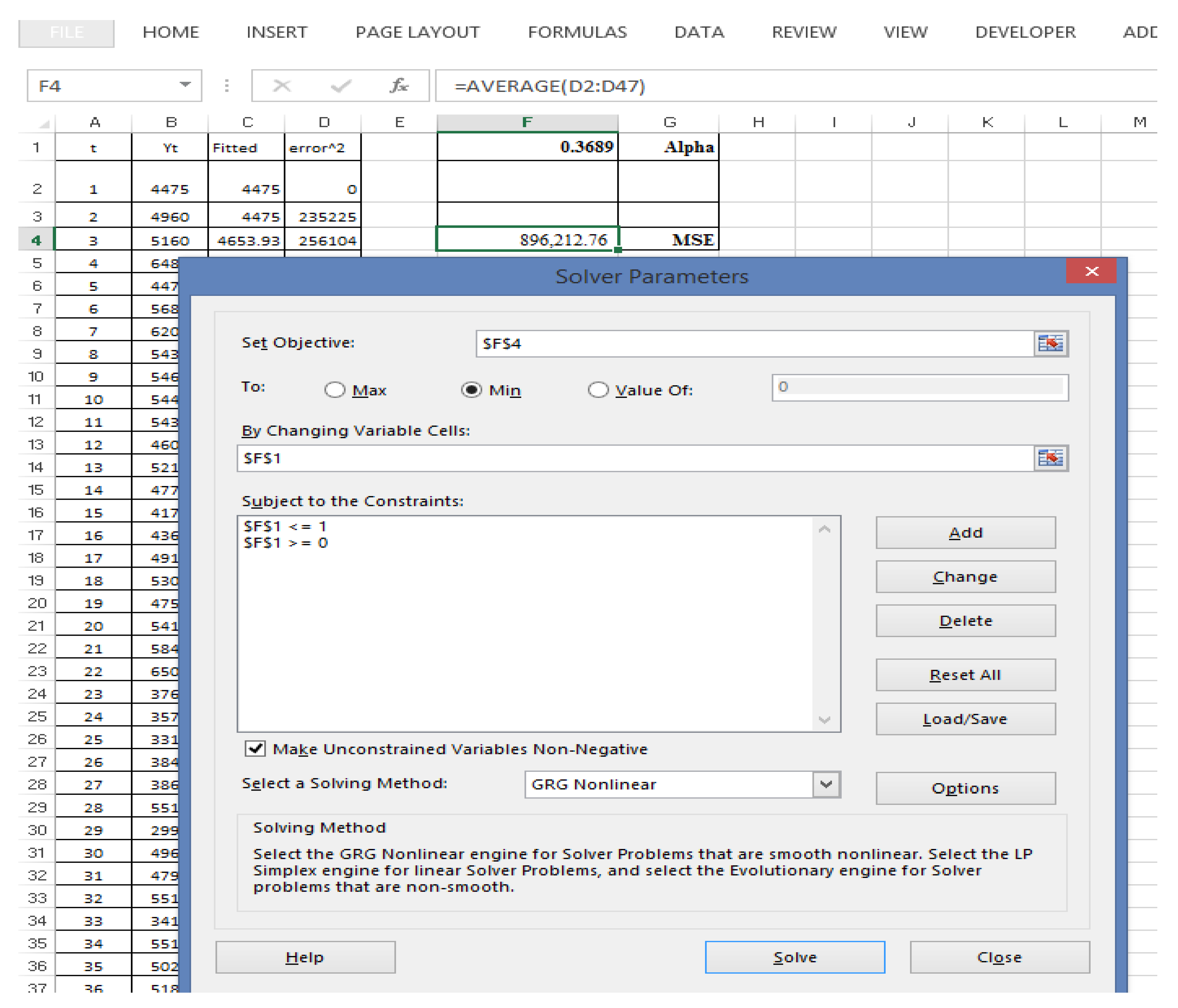
Table 3 provides the initial values via the three methods and the optimal value for α using a step search and Solver in Microsoft Excel, which were very similar. As an example for a small-sized dataset (S1), the optimal values for α using a step search and Solver from Microsoft Excel were 0.369 and 0.3689, respectively, when setting the initial value using Method 1, whereas they were 0.316 and 0.3162, respectively, when setting the initial value using Method 2, and 0.323 and 0.3232, respectively, when setting the initial value using the proposed method. This trend was the same for all of the datasets.
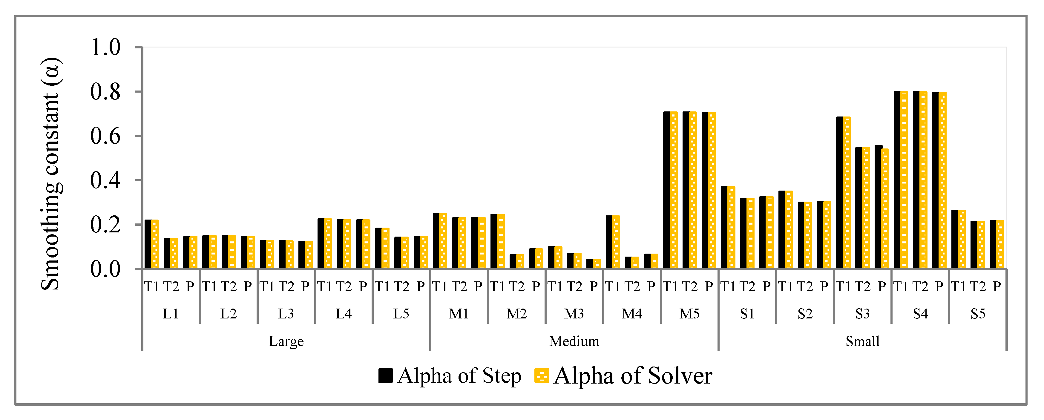
Figure 2 shows the results for each dataset when using different initialization methods; the optimal value for α differs only slightly. Eventually, Solver from Microsoft Excel and the step search methods obtained very similar optimal values for α for the same initialization method. Overall, the different sizes of small with S1–S5, medium with M1–M5, and large with L1–L5 datasets are represented by the bar chart of
Figure 3, and it can be seen that both Solver in Microsoft Excel and step search obtained nearly the same optimal value for α results. Hence, the Solver from Microsoft Excel is an alternative to a powerful method for obtaining the optimal value for α.
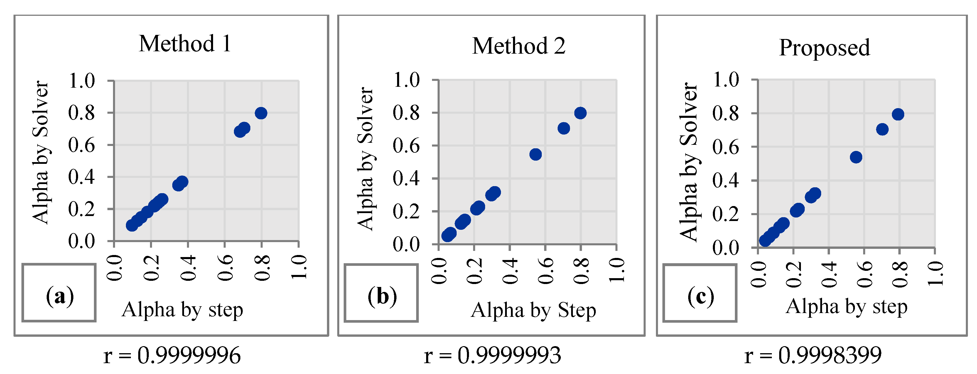
The results of a correlation analysis of the performances of the three methods are presented in
Figure 3. It can be seen that the correlation coefficient values are close to +1 and lie in a straight line, meaning that the optimal values for α obtained using the step search method or Solver from Microsoft Excel using the initial value from all three methods are in good agreement.
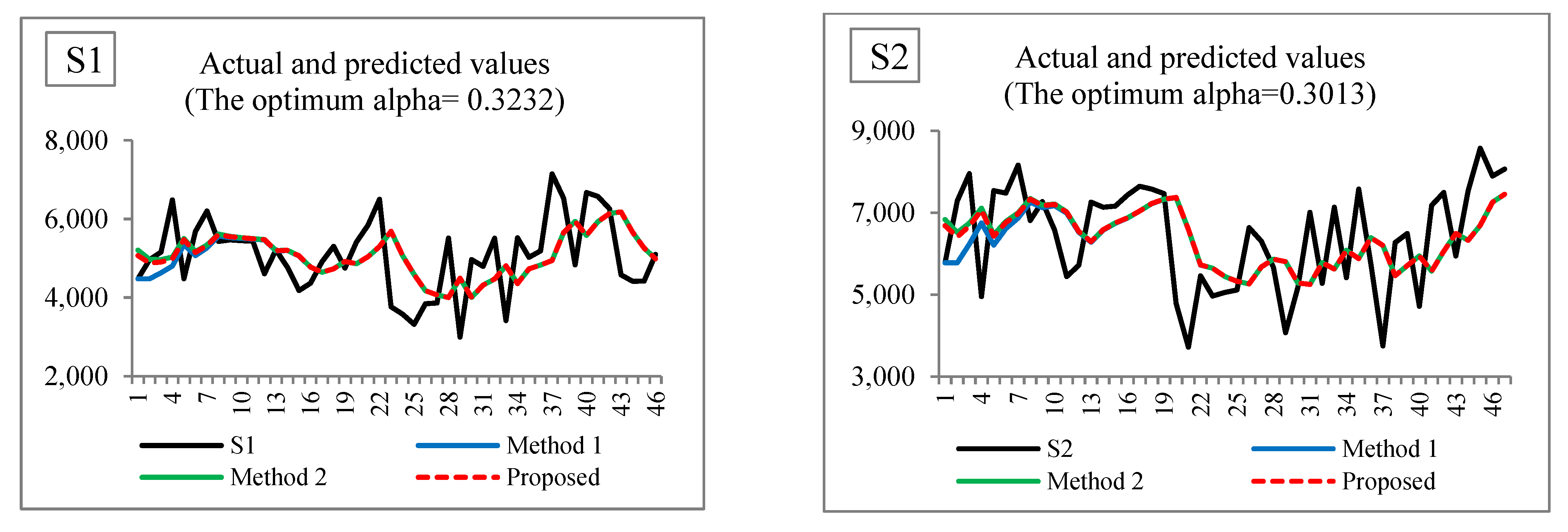
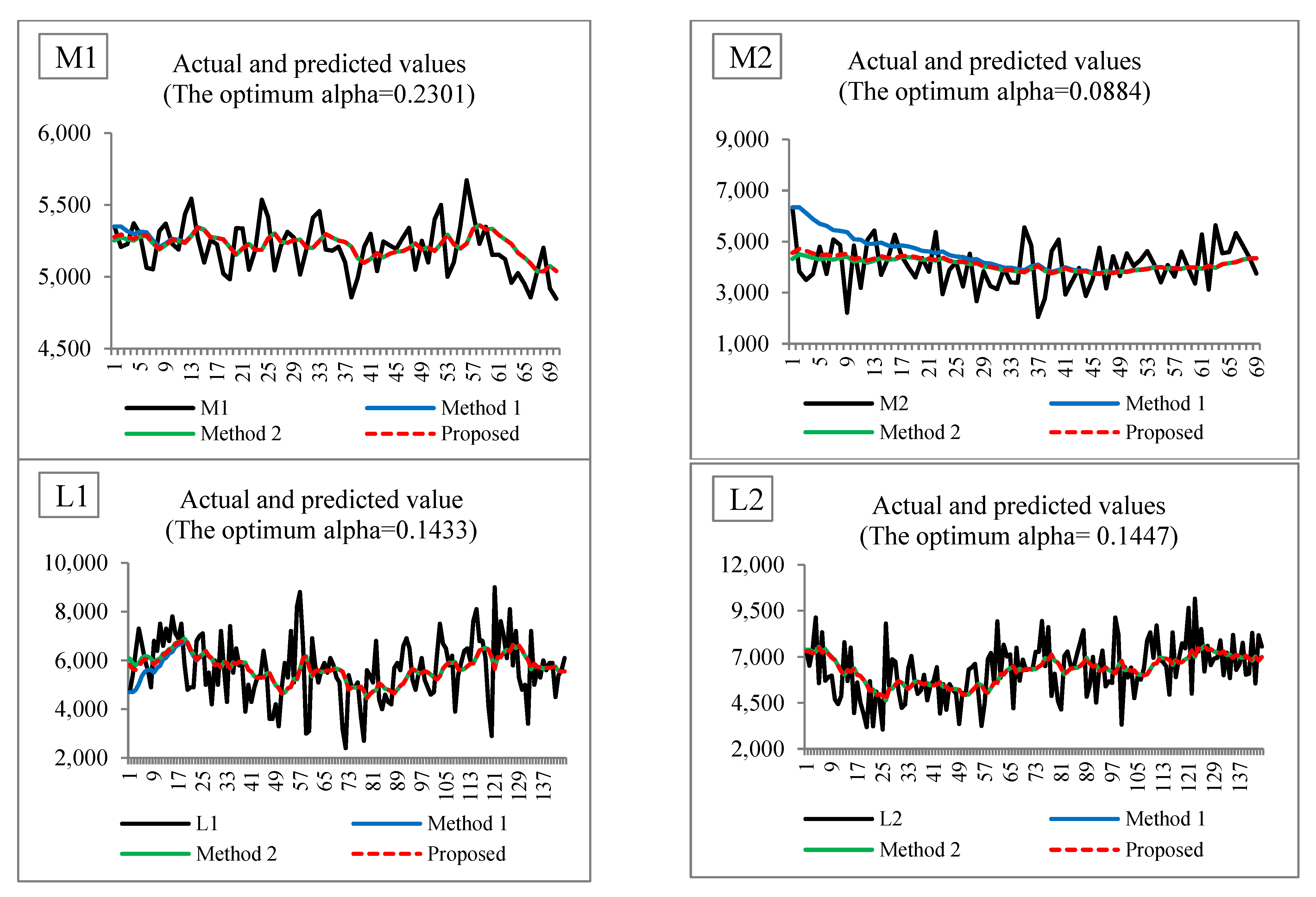
Figure 4 illustrates the actual and predicted values when setting the initial value using Method 1, Method 2, and the proposed method. For example, in S1, when setting the initial value using Method 2 and the proposed method, similar predicted values are achieved, but when setting the initial value using Method 1, the predicted values in the early period are far from those of the other methods. Additionally, they can be interpreted in the same way in the other time series. Moreover,
Table 4 reports the lowest MSE values for the three initial value setting methods used to obtain the optimal value for α using the step search method and Solver from Microsoft Excel. For each dataset, the lowest MSE value was obtained from a set of 1000 MSE values. For example, for S1, when setting the initial value using Method 1, Method 2, and the proposed method, the lowest MSE values were 896,212.77, 886,047.38, and 885,070.96, respectively. This trend was the same for the other datasets. It can be seen that although the results are similar, setting the initial value using the proposed method obtained lower MSE values than the other methods.
Figure 5 visually supports these findings.
The initial setting methods’ lowest MSE frequencies were compared using Chi-squared goodness-of-fit tests (
Table 5). The null hypothesis states that the number of times that each method achieves the lowest MSE is the same. For example, for S1, the Chi-squared statistic for the lowest MSE value is 159.65 with a
p-value < 0.0001, which leads to the conclusion that the number of times that each method achieves the lowest MSE is significantly different. The results for the other datasets can be interpreted in the same way. Thus, the proposed method for setting the initial value achieved the lowest MSE values, and it is evident that it quite considerably outperformed the other two methods.
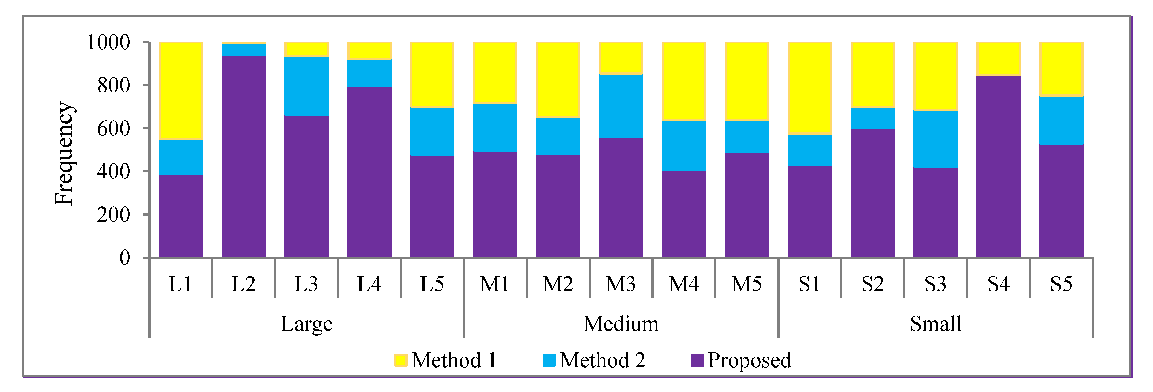
Figure 6 shows a stacked bar chart of the frequencies of obtaining the lowest MSE value when setting the initial value using the three initial value methods: Method 1, Method 2, and the proposed method for each of the 15 datasets. Notably,
Figure 6 shows the MSE values for the proposed method were lower than those for the other two methods, a trend that was the same for all of the datasets. Moreover, in
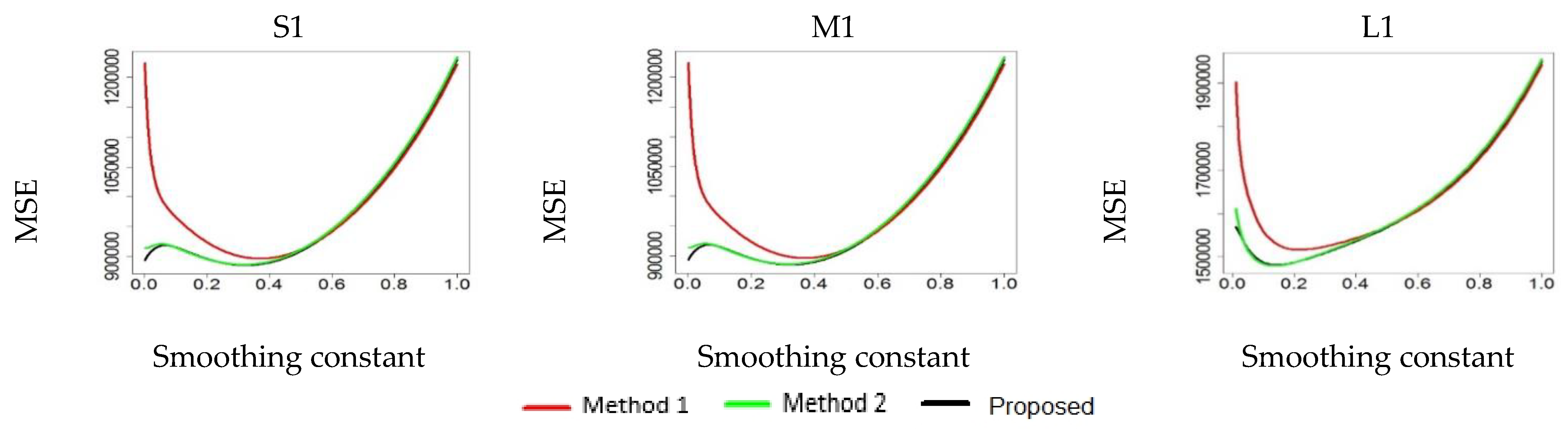
Figure 7, it is worth noting that using an initial value, in Method 1, of α in the range of 0.1–0.4 provided forecasted values far from the actual values, whereas when it exceeded 0.5, all three methods provided similar results. The proposed method and Method 2 usually provided similar MSE values for the same set of conditions, and their plotted lines tended to overlap each other. Meanwhile, lower MSE values for the three initial value setting methods became more evident as the settings were decreased. These results are consistent with the other findings, and it was concluded that the proposed method performed better than the others.
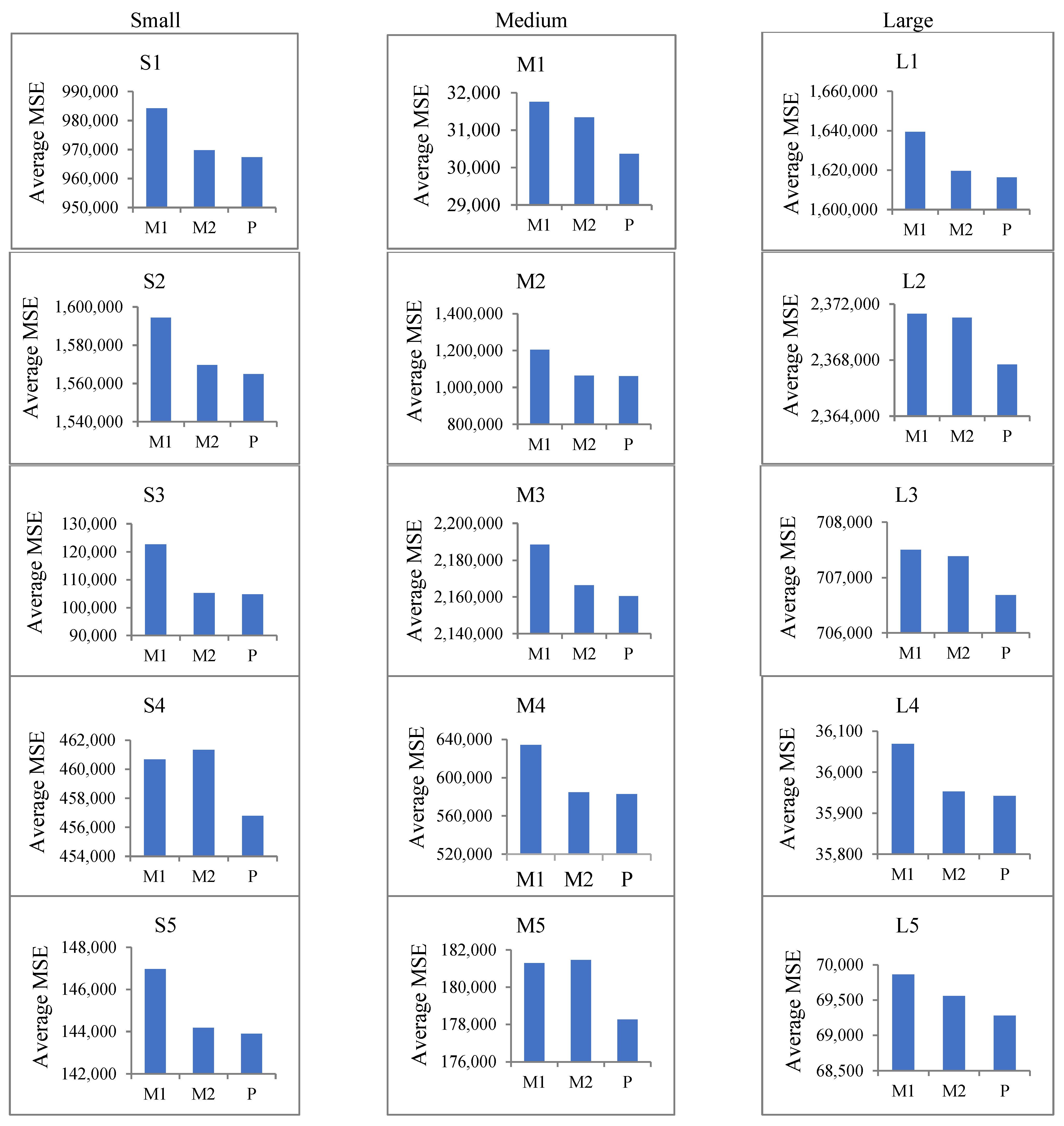
It can be seen that when using values of α ranging from 0 to 1 (0.001, 0.002, …, and 1) to produce 1000 settings, different average MSE levels were provided (
Table 6). For example, for S1, Method 1, Method 2, and the proposed method produced MSE values of 984,214.12, 969,740.55, and 967,322.56, respectively. Similarly, they produced MSE values of 31,757.83, 31,338.43, and 30,365.02, respectively, for M1, and 1,639,370.09, 1,619,541.12, and 1,616,325.69, respectively, for L1. Thus, it can be concluded that, when using the same value of 𝛼, the initial value provided by the proposed method provided the lowest MSE for all sizes of datasets and quite considerably outperformed the other two methods in this endeavor. Bar charts of the average MSE values obtained using the three methods for each dataset are shown in
Figure 8. The results clearly show that the proposed method performed much better than Method 1 and Method 2.
6. Conclusions and Remarks
To effectively use the SES method, the forecaster must first choose a proper value for α and then set the initial value to calculate the smoothed values and make the forecast. The MSE is often used as a criterion for selecting an appropriate value for α. For instance, by assigning the values [0,1], one then selects the value that produces the smallest MSE. Importantly, these values considerably affect the accuracy of the forecast.
In this study, the Solver in Microsoft Excel and step search methods were used to determine the value of α that optimally fitted several time series datasets. Since their performances were not different, Solver from Microsoft Excel is a powerful alternative method for obtaining the optimal value for α. Moreover, the initial value influenced the forecast using the SES method. The simple initial value setting using the first observed value provided a far worse performance than the other two methods based on small, medium, and large time series datasets. It is worth noting that using values for α in the range 0.1–0.4 as the initial value with the first observed provided forecasted values far from the actual value, whereas when it exceeded 0.5, all three methods provided similar results. The limitation of SES work is based on the principle that a prediction is a weighted linear sum of past observations. Moreover, the forecasting accuracy is directly affected by the value of α since it adjusts the weights given to observations and the initial value. Therefore, it is always important to choose a proper value for α.


