
Multiscale Design of Graded Stochastic Cellular Structures for the Heat Transfer Problem


Abstract
:1. Introduction
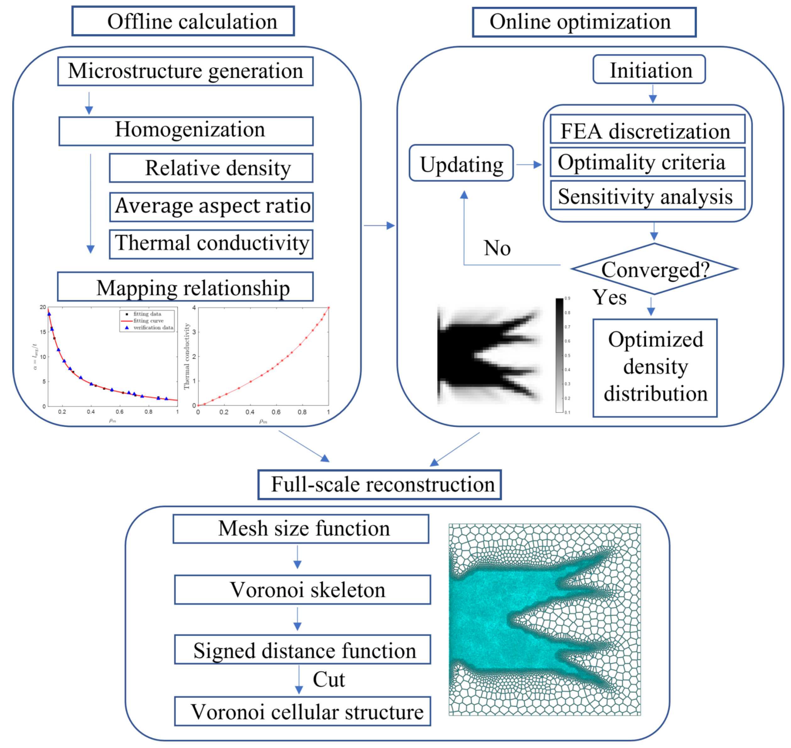
2. Methodology
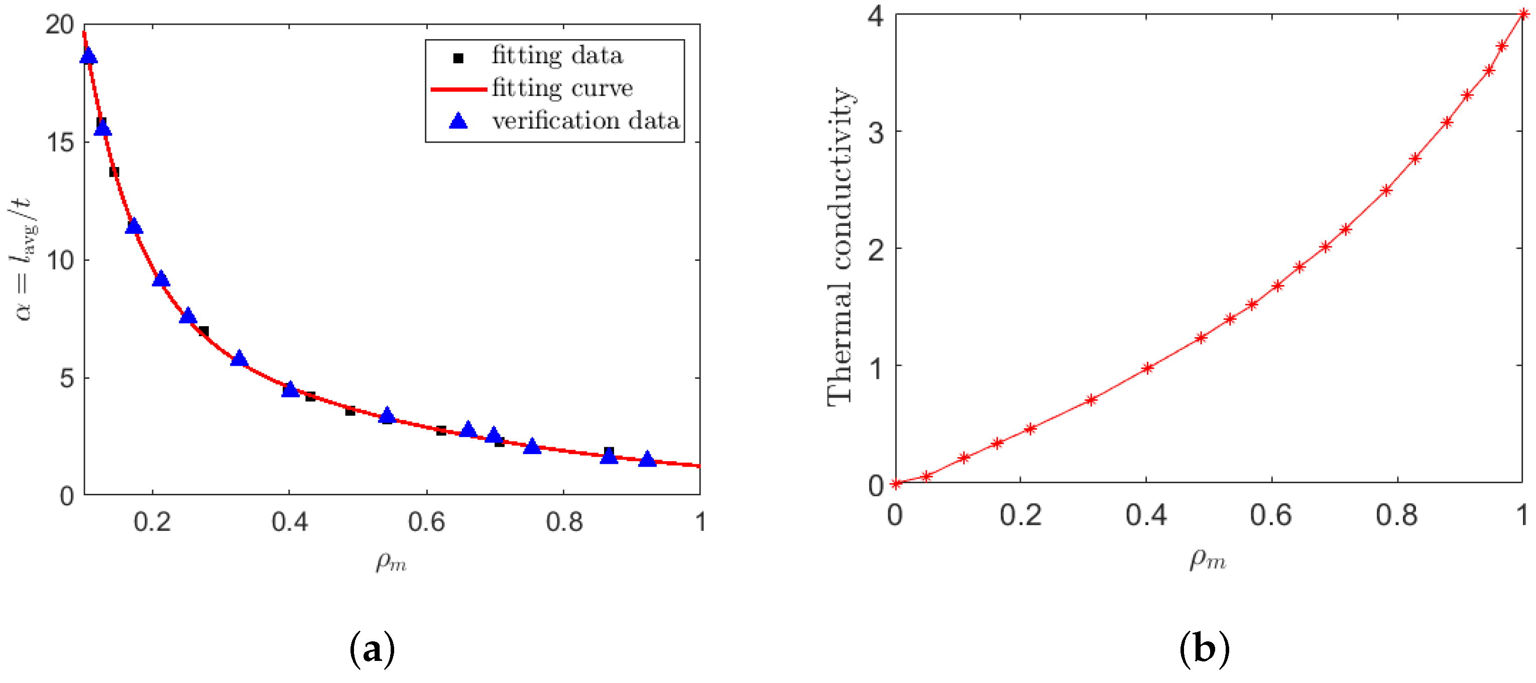
2.1. Offline Calculation on the Microscale
2.2. Online Optimization on the Macroscale
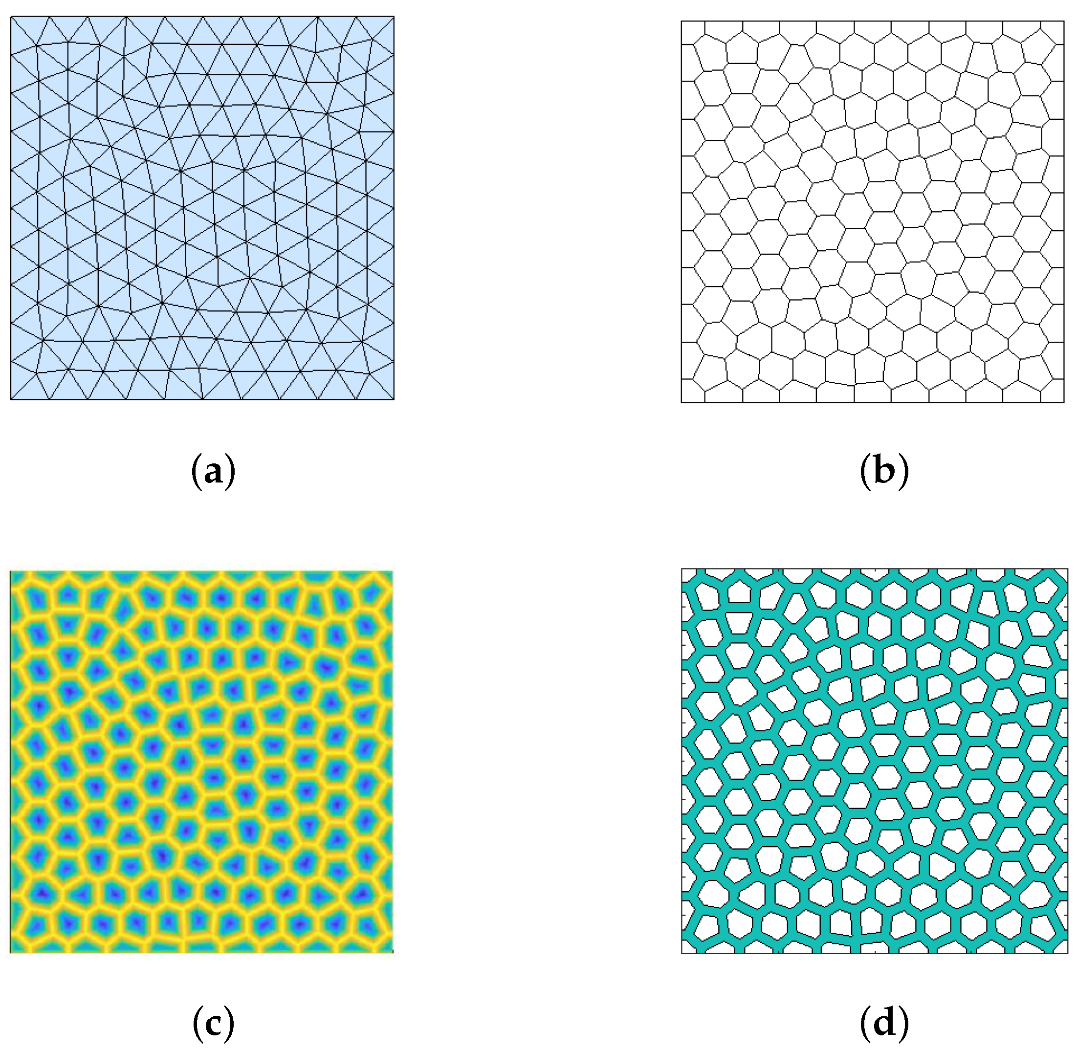
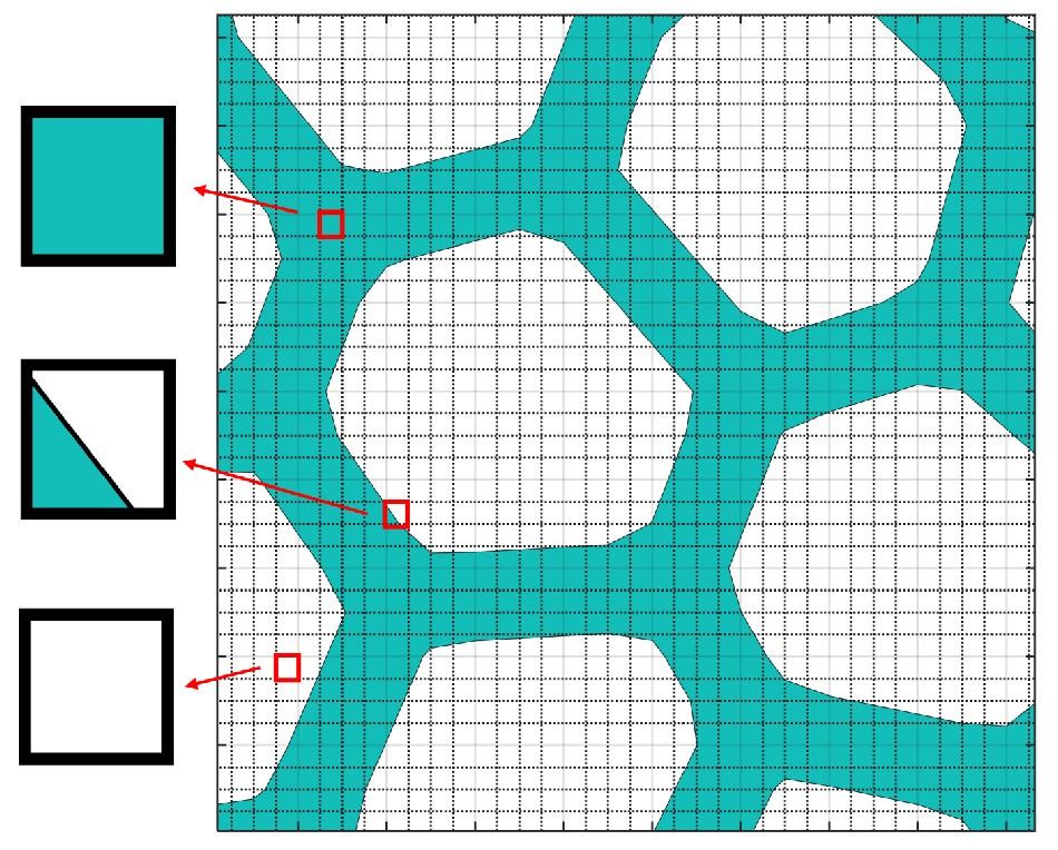
2.3. Geometry Reconstruction on the Full-Scale
3. Numerical Examples
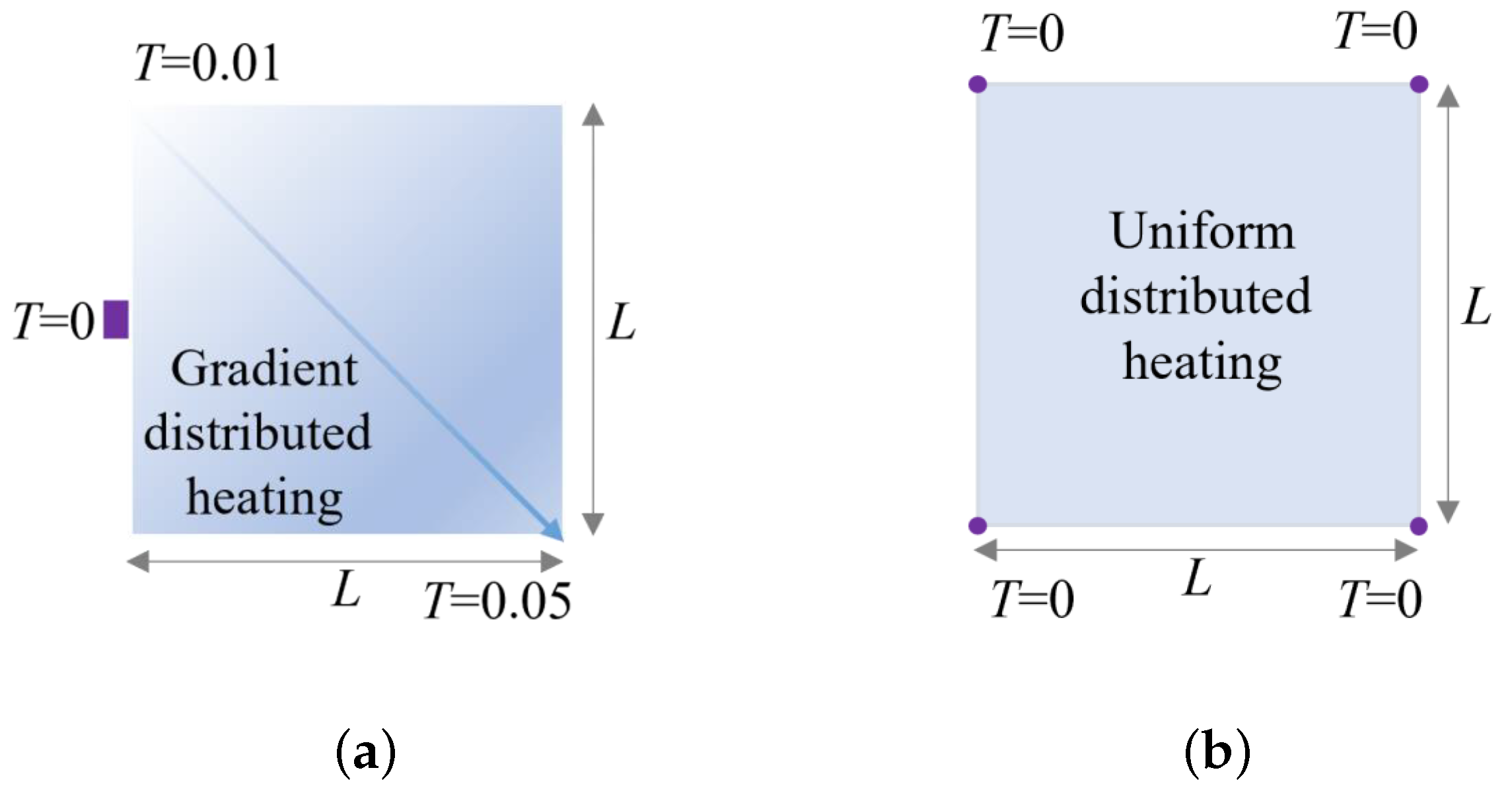
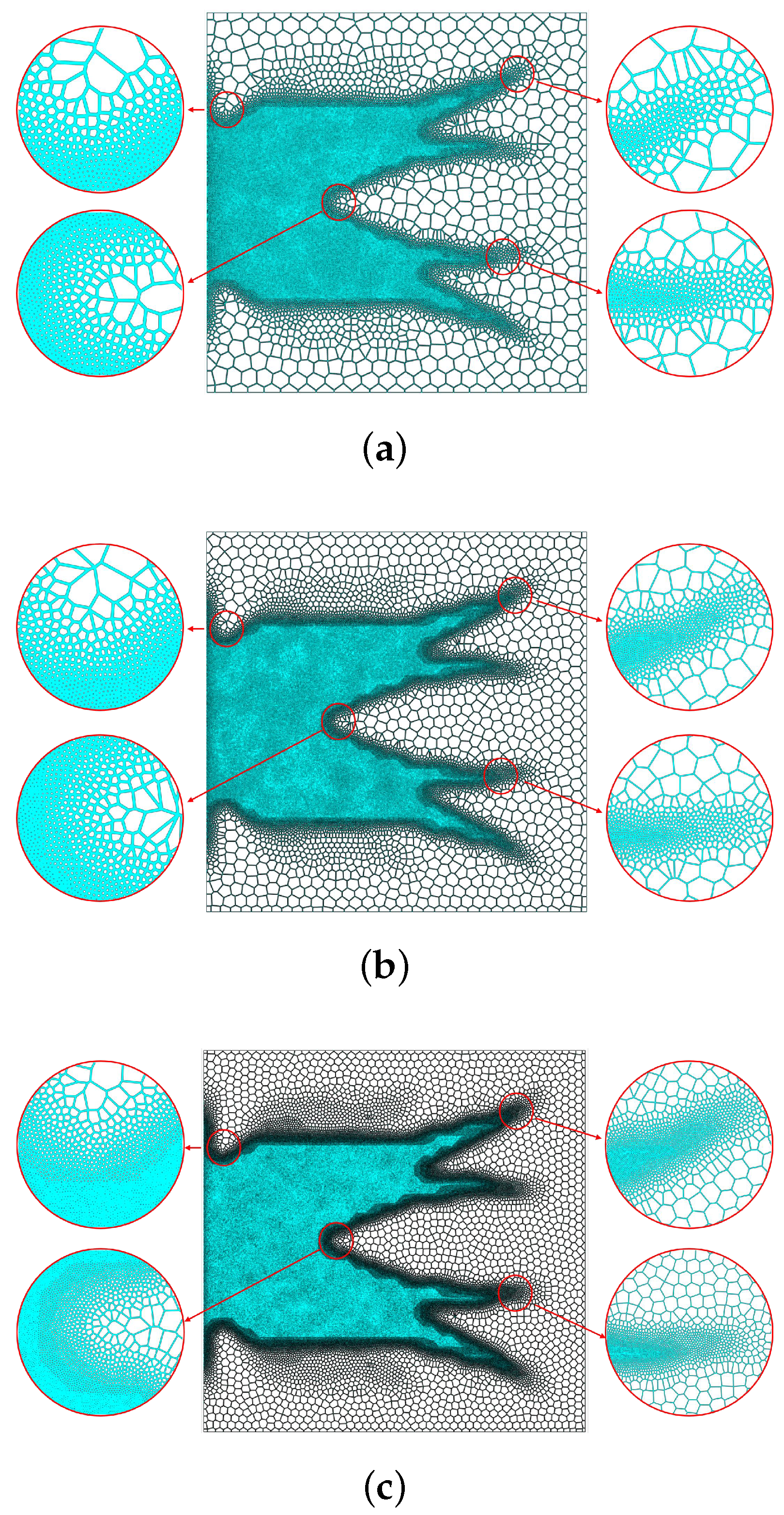
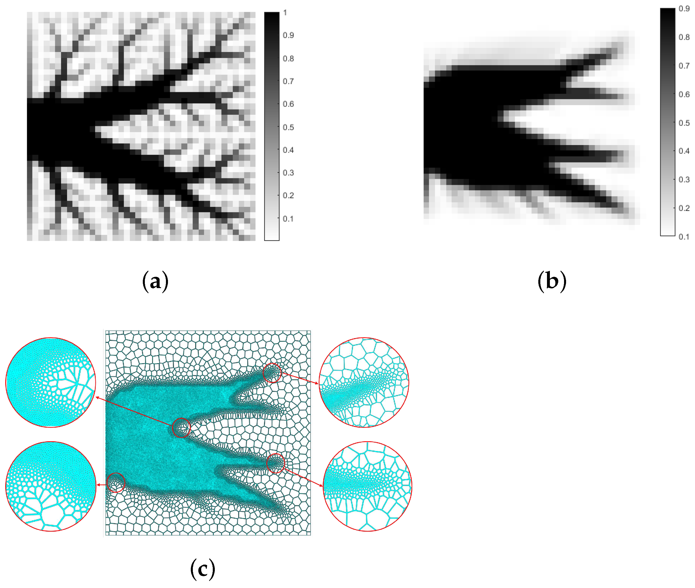
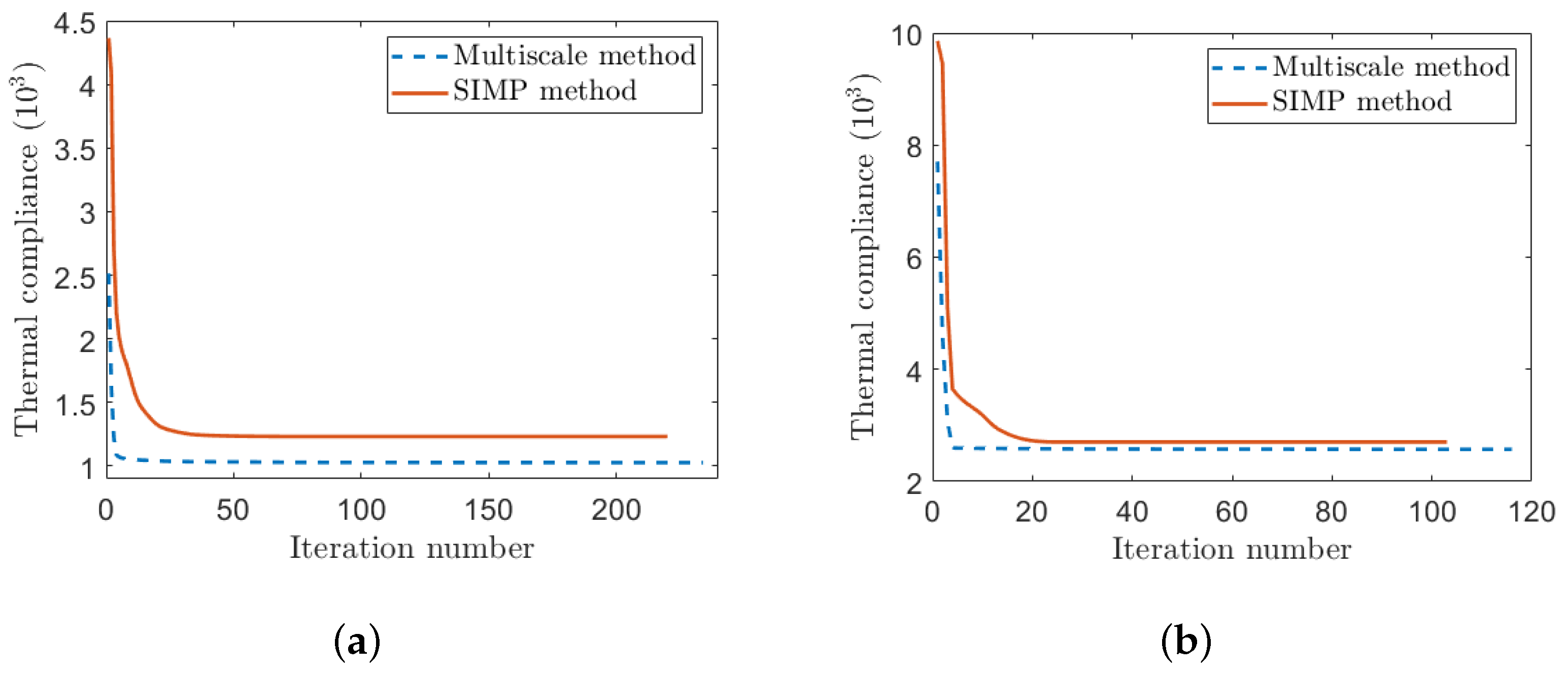
3.1. 2D Benchmark Example
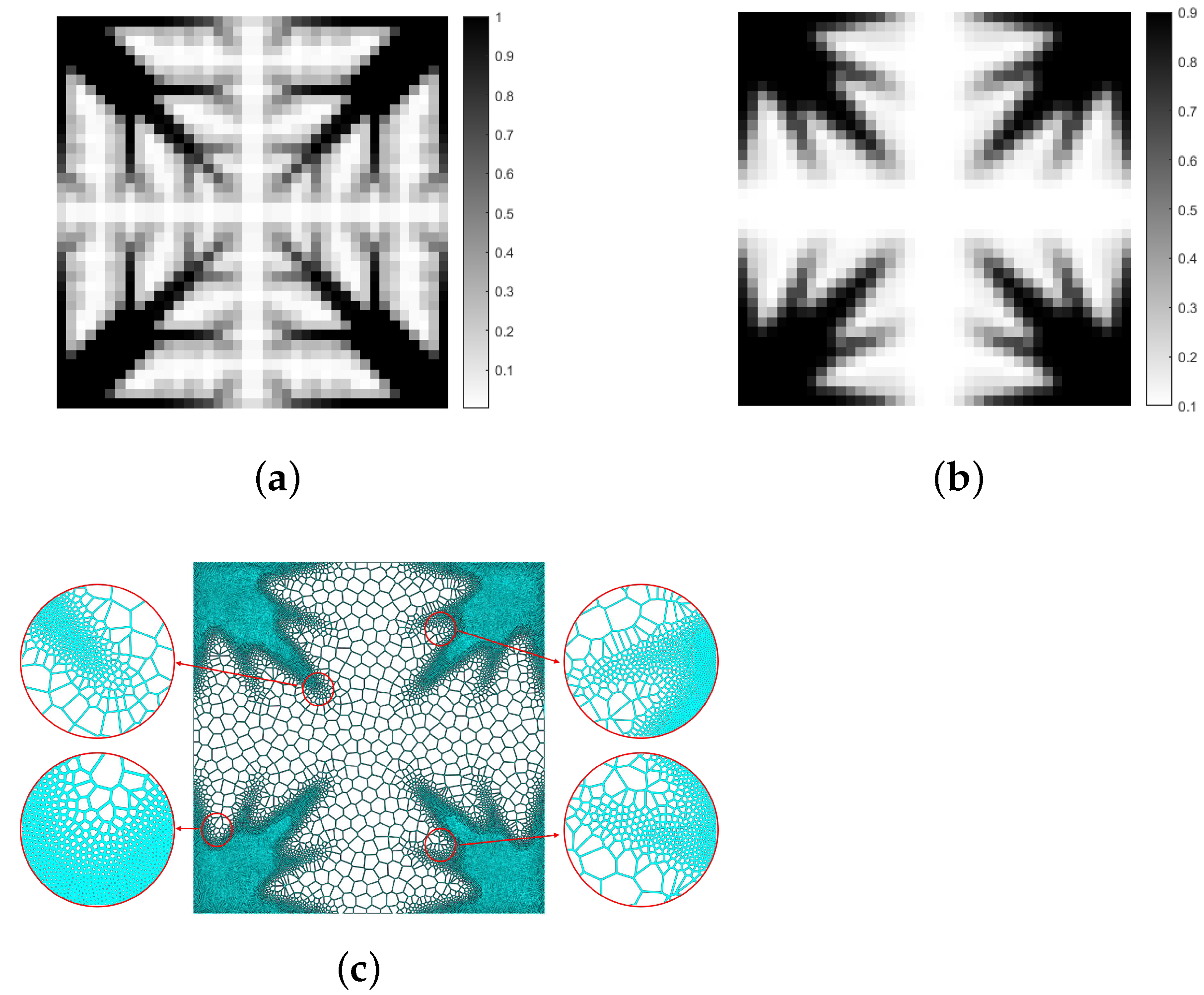
3.2. Extensive Numerical Examples
4. Conclusions
Author Contributions
Funding
Institutional Review Board Statement
Informed Consent Statement
Data Availability Statement
Conflicts of Interest
References
- Liu, J.; Gaynor, A.T.; Chen, S.; Kang, Z.; Suresh, K.; Takezawa, A.; Li, L.; Kato, J.; Tang, J.; Wang, C.C.L.; et al. Current and future trends in topology optimization for additive manufacturing. Struct. Multidiscip. Optim. 2018, 57, 2457–2483. [Google Scholar] [CrossRef] [Green Version]
- Hassani, B.; Hinton, E. A review of homogenization and topology optimization i homogenization theory for media with periodic structure. Comput. Struct. 1998, 69, 707–717. [Google Scholar] [CrossRef]
- Hassani, B.; Hinton, E. A review of homogenization and topology opimization ii analytical and numerical solution of homogenization equations. Comput. Struct. 1998, 69, 719–738. [Google Scholar] [CrossRef]
- Wu, J.; Aage, N.; Westermann, R.; Sigmund, O. Infill optimization for additive manufacturing—Approaching bone-like porous structures. IEEE Trans. Vis. Comput. Graph. 2016, 24, 57–107. [Google Scholar] [CrossRef] [PubMed] [Green Version]
- Liu, C.; Du, Z.; Zhang, W.; Zhu, Y.; Guo, X. Additive manufacturing oriented design of graded lattice structures through explicit topology optimization. J. Appl. Mech. 2017, 84, 081008. [Google Scholar] [CrossRef]
- Zong, H.M.; Liu, H.; Ma, Q.P.; Tian, Y.; Zhou, M.D.; Michael, Y.W. Vcut level set method for topology optimization of functionally graded cellular structures. Comput. Methods Appl. Mech. Eng. 2019, 354, 487–505. [Google Scholar] [CrossRef]
- Liu, H.; Zong, H.M.; Shi, T.L.; Qi, X. Mvcut level set method for optimizing cellular structures. Comput. Methods Appl. Mech. Eng. 2020, 367, 113–154. [Google Scholar] [CrossRef]
- Xia, Q.; Zong, H.M.; Shi, T.L.; Liu, H. Optimizing cellular structures through the mvcut level set method with microstructure mapping and high order cutting. Compos. Struct. 2020, 261, 113298. [Google Scholar] [CrossRef]
- Liu, H.; Zong, H.M.; Tian, Y.; Ma, Q.P.; Michael, Y.W. A novel subdomain level set method for structural topology optimization and its application in graded cellular structure design. Struct. Multidiscip. Optim. 2019, 60, 2221–2247. [Google Scholar] [CrossRef]
- Xia, L.; Breitkopf, P. Concurrent topology optimization design of material and structure within FE2 nonlinear multiscale analysis framework. Comput. Methods Appl. Mech. Eng. 2014, 278, 524–542. [Google Scholar] [CrossRef]
- Rodrigues, H.; Guedes, J.M.; Bendsoe, M.P. Hierarchical optimization of material and structure. Struct. Multidiplinary Optim. 2002, 24, 1–10. [Google Scholar] [CrossRef]
- Wu, J.; Wang, W.M.; Gao, X.F. Design and optimization of conforming lattice structures. IEEE Trans. Vis. Comput. Graph. 2021, 27, 43–56. [Google Scholar] [CrossRef] [Green Version]
- Groen, J.P.; Wu, J.; Sigmund, O. Homogenization based stiffness optimization and projection of 2d coated structures with orthotropic infill. Comput. Methods Appl. Mech. Eng. 2019, 349, 722–742. [Google Scholar] [CrossRef]
- Groen, J.P.; Sigmund, O. Homogenization based topology optimization for highresolution manufacturable microstructures. Int. J. Numer. Methods Eng. 2018, 113, 1148–1163. [Google Scholar] [CrossRef] [Green Version]
- Chen, W.J.; Tong, L.Y.; Liu, S.T. Concurrent topology design of structure and material using a twoscale topology optimization. Comput. Struct. 2017, 178, 119–128. [Google Scholar] [CrossRef]
- Sigmund, O. A 99 line topology optimization code written in Matlab. Struct. Multidiscip. Optim. 2001, 21, 120–127. [Google Scholar] [CrossRef]
- Xie, Y.; Steven, G.P. A simple evolutionary procedure for structural optimization. Comput. Struct. 1993, 49, 885–896. [Google Scholar] [CrossRef]
- Wang, M.Y.; Wang, X.; Guo, D. A level set method for structural topology optimization. Comput. Methods Appl. Mech. Eng. 2003, 192, 227–246. [Google Scholar] [CrossRef]
- Guo, X.; Zhang, W.; Zhong, W. Doing topology optimization explicitly and geometrically—A new moving morphable components based framework. J. Appl. Mech. 2014, 81, 081009. [Google Scholar] [CrossRef]
- Olhoff, N. Optimization of vibrating beams with respect to higher order natural frequencies. J. Struct. Mech. 1976, 4, 87–122. [Google Scholar] [CrossRef]
- Xie, Y.; Steven, G.P. Evolutionary structural optimization for dynamic problems. Comput. Struct. 1996, 58, 1067–1073. [Google Scholar] [CrossRef]
- Xia, Q.; Shi, T.; Wang, M.Y. A level set based shape and topology optimization method for maximizing the simple or repeated first eigenvalue of structure vibration. Struct. Multidiscip. Optim. 2011, 43, 473–485. [Google Scholar] [CrossRef]
- Niu, B.; Yan, J.; Cheng, G. Optimum structure with homogeneous optimum cellular material for maximum fundamental frequency. Struct. Multidiscip. Optim. 2009, 39, 115–132. [Google Scholar] [CrossRef]
- Liu, H.B.H.; Chen, L. Data-driven m-vcut topology optimization method for heat conduction problem of cellular structure with multiple microstructure prototypes. Int. J. Heat Mass Transf. 2022, 198, 123421. [Google Scholar] [CrossRef]
- Montemurro, M.; Refai, K.; Catapano, A. Thermal design of graded architected cellular materials through a cad-compatible topology optimisation method. Compos. Struct. 2021, 280, 124862. [Google Scholar] [CrossRef]
- Imediegwu, C.; Murphy, R.; Hewson, R.; Santer, M. Multiscale thermal and thermostructural optimization of three-dimensional lattice structures. Struct. Multidiplinary Optim. 2021, 65, 13. [Google Scholar] [CrossRef]
- Cheng, L.; Liu, J.; Liang, X.; To, A.C. Coupling lattice structure topology optimization with design-dependent feature evolution for additive manufactured heat conduction design. Comput. Methods Appl. Mech. Eng. 2018, 332, 408–439. [Google Scholar] [CrossRef]
- Lu, W.F.; Han, Y.F. A novel design method for nonuniform lattice structures based on topology optimization. J. Mech. Des. 2018, 140, 091403. [Google Scholar]
- Gomez, S.; Vlad, M.D.; Lopez, J.; Fernandez, E. Design and properties of 3d scaffolds for bone tissue engineering. Acta Biomater. 2016, 42, 341–350. [Google Scholar] [CrossRef]
- Martinez, J.; Dumas, J.; Lefebvre, S. Procedural voronoi foams for additive manufacturing. ACM Trans. Graph. 2016, 35, 1–12. [Google Scholar] [CrossRef] [Green Version]
- Martinez, J.; Hornus, S.; Song, H.C.; Lefebvre, S. Polyhedral voronoi diagrams for additive manufacturing. ACM Trans. Graph. 2018, 37, 1–15. [Google Scholar] [CrossRef] [Green Version]
- Lei, H.Y.; Li, J.R.; Xu, Z.J.; Wang, Q.H. Parametric design of voronoi based lattice porous structures. Mater. Des. 2020, 191, 108607. [Google Scholar] [CrossRef]
- Do, Q.T.; Nguyen, C.H.P.; Choi, Y. Homogenization-based optimum design of additively manufactured voronoi cellular structures. Addit. Manuf. 2022, 45, 102057. [Google Scholar] [CrossRef]
- Persson, P.O.; Strang, G. A simple mesh generator in matlab. Siam Rev. 2004, 46, 329–345. [Google Scholar] [CrossRef] [Green Version]
- Talischi, C.; Paulino, G.H.; Pereira, A.; Menezes, L.F.M. Polymesher: A generalpurpose mesh generator for polygonal elements written in matlab. Struct. Multidiscip. Optim. 2012, 45, 309–328. [Google Scholar] [CrossRef]
- Cao, S.H.; Greenhalgh, S. Finitedifference solution of the eikonal equation using an efficient, firstarrival, wavefront tracking scheme. Grophysics 1994, 59, 632–643. [Google Scholar] [CrossRef]
- Andreassen, E.; Andreasen, C.S. How to determine composite material properties using numerical homogenization. Comput. Mater. Sci. 2014, 83, 488–495. [Google Scholar] [CrossRef] [Green Version]
- Bendsøe, M.P.; Sigmund, O. Optimization of Structural Topology, Shape, and Materials; Springer: Berlin/Heidelberg, Germany, 1998. [Google Scholar]
- Andreassen, E.; Clausen, A.; Schevenels, M.; Lazarov, B.S.; Sigmund, O. Efficient topology optimization in matlab using 88 lines of code. Struct. Multidiscip. Optim. 2011, 43, 1–16. [Google Scholar] [CrossRef] [Green Version]


| Microstructure | ||
|---|---|---|
 |
| a | b | c | d |
|---|---|---|---|
| 43.67 | −13.42 | 10.08 | −2.11 |
Disclaimer/Publisher’s Note: The statements, opinions and data contained in all publications are solely those of the individual author(s) and contributor(s) and not of MDPI and/or the editor(s). MDPI and/or the editor(s) disclaim responsibility for any injury to people or property resulting from any ideas, methods, instructions or products referred to in the content. |
© 2023 by the authors. Licensee MDPI, Basel, Switzerland. This article is an open access article distributed under the terms and conditions of the Creative Commons Attribution (CC BY) license (https://creativecommons.org/licenses/by/4.0/).
Share and Cite
Chen, L.; Zhang, R.; Chu, X.; Liu, H. Multiscale Design of Graded Stochastic Cellular Structures for the Heat Transfer Problem. Appl. Sci. 2023, 13, 4409. https://doi.org/10.3390/app13074409
Chen L, Zhang R, Chu X, Liu H. Multiscale Design of Graded Stochastic Cellular Structures for the Heat Transfer Problem. Applied Sciences. 2023; 13(7):4409. https://doi.org/10.3390/app13074409
Chicago/Turabian StyleChen, Lianxiong, Ran Zhang, Xihua Chu, and Hui Liu. 2023. "Multiscale Design of Graded Stochastic Cellular Structures for the Heat Transfer Problem" Applied Sciences 13, no. 7: 4409. https://doi.org/10.3390/app13074409