Abstract
For the trajectory optimization of the time–jerk of robotic arms with a chicken swarm optimization algorithm, using five-order B-spline interpolation can ensure smooth and continuous acceleration, but, due to the performance problems of the algorithm, the low solution accuracy and the slow convergence speed, the ideal trajectory curve cannot be obtained. To address these problems, an improved chicken swarm algorithm based on a parallel strategy and dynamic constraints (PDCSO) is proposed, where the rooster update method is employed with a parallel strategy using X-best guidance and a Levy flight step. Dynamic constraints for the rooster are given, followed by the hens, and the optimal rooster position that improved the convergence accuracy while preventing the local optimum was determined. Simulation experiments using 18 classical test functions showed that the PDCSO algorithm outperformed other comparative algorithms in terms of convergence speed, solution accuracy and solution stability. Simulation validation in ADAMS and real machine tests proved that PDCSO can effectively reduce the running time and motion shock for robotic arms and improve the execution efficiency of such arms.
1. Introduction
Trajectory planning is the basis of robot motion control and is related to the stability of robot motion, work efficiency, energy consumption, etc. [1,2,3,4]. Robot trajectory planning determining the trajectory of the end movement of a robotic arm to meet process requirements and ensure high performance links the space and time domains of the robot in the process of movement [5]. Optimized trajectory planning can help meet process requirements, reduce quick jerk and improve construction quality to enable smooth motion. For example, Peng et al. [6] used a non-dominated neighborhood immune genetic algorithm to optimize the multi-objective trajectory function for a robot. They determined the optimal position, velocity, acceleration and acceleration planning curves for each joint of the robot. Huang et al. [7] used five-order B-spline interpolation to interpolate the trajectory in the joint space. They then used an elite non-dominated ranking genetic algorithm (NSGA-II) to optimize the two objectives—i.e., motion time and average acceleration—for the entire trajectory. Zhang et al. [8] carried out time–jerk optimal trajectory planning for an excavator using an SQP algorithm with the constraints of joint angular velocity, angular acceleration and angular acceleration by interpolating in the joint space using three-order B-spline interpolation. Du et al. [9] proposed a method based on a segmented polynomial interpolation function and the local chaotic particle swarm optimization (LCPSO) algorithm to achieve robotic-arm time optimality.
Different trajectory planning methods can achieve different planning effects, and among the many planning algorithms, the B-spline curve [10] has outstanding advantages: its trajectory is smooth and can guarantee velocity, acceleration and acceleration continuity simultaneously; however, it requires substantial computational power compared to other methods. At the same time, single optimal trajectory planning methods cannot meet the comprehensive requirements of modern industrial applications. The integrated consideration of two or more optimality methods is more suitable for trajectory planning in practical applications [11]. Complex planning methods and multi-objective optimization require large amounts of computational power and consideration of the complex constraints brought about by actual working conditions, all of which place higher demands on the accuracy and speed with which the solution is obtained in the optimization algorithm.
Chicken swarm optimization (CSO), proposed by Meng et al. [12], is a novel swarm intelligence optimization algorithm. It can be used to optimize various specific problems by simulating the intelligent behavior of a swarm composed of roosters, hens and chicks foraging for food. The chicken swarm optimization algorithm has a clear structure and robust searching ability, as well as being easy to understand and implement. Additionally, it has better convergence than the particle swarm algorithm, differential evolution algorithm and artificial bee swarm algorithm [12]. It has several research applications, such as task scheduling, route optimization, etc. [13], but suffers from the problem of falling into local optimality, leading to premature maturity and a low solution accuracy. To address the issues of the CSO algorithm, researchers have proposed improvement methods. Irsalinda et al. [14] proposed a multi-stage CSO algorithm based on the search characteristics of different chickens. In the first stage, the algorithm focuses on the hen update method to strengthen the global exploration ability; in the second stage, the algorithm focuses on the chick and rooster update methods to reflect the advantage of local exploitation. Zhang [15] proposed an improved CSO algorithm based on forward- and backward-learning rooster particles, allowing it to positively learn from the optimal particles in each iteration so that the algorithm can quickly enter the most promising region to find food while learning backward from the worst particles to jump out of the local optimum when the algorithm is stuck in the local optimum solution. Zhang et al. [16] proposed improvements using X-best bootstrap individuals and a dynamic rank update mechanism. The best individuals were introduced to accelerate the convergence in the individual update phase, and the influence of ordinary individuals on the best individuals was properly balanced. Additionally, the contribution of the population rank update mechanism to the algorithm convergence was enhanced through dynamic optimization of the rank update parameters. Gu et al. [17] removed the chicks, simplified the algorithm, proposed an improved update for both males and females based on inverted s-shaped inertia rights and added an adaptive update strategy to the update process for females. Liang et al. [18] introduced an improved search strategy with Levy flight characteristics into the location update equation for hens, helping to increase the algorithm’s perturbation and population diversity. Secondly, a nonlinear decreasing strategy was added to the chicken position update equation to improve the chickens’ self-learning ability.
In this paper, in order to improve the convergence accuracy and convergence speed of the CSO algorithm using time–jerk trajectory optimization, a parallel strategy was employed for the rooster update method while introducing X-best guidance and a Levy flight step; dynamic constraints were developed for the rooster followed by the hen, and the optimal rooster following position was introduced to improve convergence accuracy while avoiding falling into local optima. The simulation results for the above algorithm proved that the proposed optimization method was effective in improving the convergence speed and convergence accuracy of the algorithm, and ADAMS simulation and real machine experiments verified that the improved algorithm can effectively reduce the running time and motion shock of the robotic arm, improve the execution efficiency of the robotic arm and lay the foundation for completing the motion control of the robotic arm.
2. Improved Chicken Swarm Algorithm
The stochastic optimization algorithm that simulates the behavioral habits of chickens and the hierarchy within the swarm is called chicken swarm optimization (CSO). The basic idea of the CSO algorithm is to classify chickens into roosters, hens and chicks according to their fitness values. Assuming a series of rules, different types of chickens follow different movement rules and compete with each other to find food. The CSO algorithm is a global optimization algorithm.
The chicken swarm algorithm employs the following rules.
In a chicken swarm, there are several groups. Each group consists of a dominant rooster and several hens and chicks.
Adaptation determines the status of the chickens (roosters, hens and chicks). Several of the best-adapted chickens will be treated as roosters, with each rooster being the lead rooster in a group. A few of the least well-adapted chickens will be designated as chicks and the others as hens. The hens randomly choose which group to live in. The mother–child relationship between the hen and the chick is also randomly established.
The hierarchical order, dominance and mother–child relationships within the group remain unchanged. These states are renewed every generations.
Each group is renewed differently, with the hens in each group following the roosters in that group to forage for food or randomly stealing food from other groups; the chicks in each group similarly follow the mother hen to forage for food.
The individual’s position corresponds to the optimization problem’s solution, and the algorithm replaces the lagging individuals from the previous generation with a new generation of outstanding individuals at each iteration.
The total number of clusters in the population is , the number of roosters is , the number of hens is , the number of chicks is and the number of mother hens is . The mother hen is chosen randomly from among the hens and has chicks that follow her.
Roosters dominate the entire foraging process and can forage across a much larger space. The rooster position update equation is as follows:
where is the Gaussian distribution with a mean of and variance ; is the small constant introduced to prevent the denominator from being incorrect; is another individual in the rooster population different from the current individual ; and is its fitness.
The updated hen location is calculated as follows:
where is a random number within ; is the rooster corresponding to the hen; and , is an individual different from randomly selected from the rooster population and the hen population.
The chick position update is calculated as follows:
where the subscript denotes the mother hen of chick , and is the coefficient of the chick following the mother hen, which has a value in the range of .
2.1. Improved CSO
The rooster occupies the dominant position in the whole population, guiding the hens and chicks toward the optimal solution. The update equation in the standard CSO algorithm is more conducive to maintaining the diversity of the population [12] but leads to a low solution accuracy and weak local solution capability. A reasonable X-best bootstrap mechanism has the advantage of improving the solution accuracy, but its unreasonable use will make individuals in the population overly dependent on X-best individuals, which in turn leads to a reduction in population diversity and increases the possibility of falling into local optimal solutions. To address this problem, many scholars have introduced the optimal global position into the rooster position update [15,16,19].
2.1.1. Parallel Policy-Based X-Best Bootstrap and Levy Flight Rooster Update Mechanism
In order to overcome the poor solution accuracy and prematurity caused by the introduction of the X-best bootstrap mechanism, this paper proposes a rooster update mechanism based on a parallel strategy involving X-best guidance and Levy flight.
First, the global and most individual bootstrap is introduced in the rooster update equation and, in order to avoid the overdependence on that causes the algorithm to fall into a local optimum, the adjustment coefficient is introduced before the term. The improved rooster update equation is as follows:
where is the position of the optimal individual in the th iteration and is the regulation coefficient.
The modulation coefficient was designed with three segments: either unreferenced, progressively referenced or fully referenced. The equation for the regulation factor is as follows:
where is the maximum number of iterations, and is the th iteration.
The unreferenced stage is , and Equation (7) is the same as the original algorithm (Equation (1)) after simplification. At this point, the rooster position update is not affected by .
The progressive reference stage is according to Equation (8), which nonlinearly increases when gradually intervenes, updating the position of the rooster.
The full reference stage is , at which point fully intervenes to update the position of the rooster.
To visualize the three stages of the modulation coefficient , as shown in Figure 1, the maximum number of iterations was set as . Additionally, it can be seen that the three unreferenced, asymptotically referenced and fully referenced segments are clearly distinguished, following the above requirements.
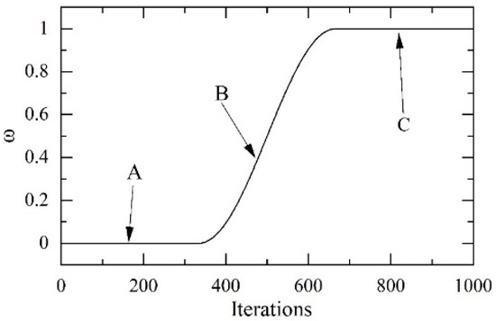
Figure 1.
modulation factor curve. A: Unreferenced stage; B: progressive reference stage; C: full reference stage.
Levy flight is a random wandering model designed according to the Levy distribution, which was proposed by the French mathematician Levy [20]. The Levy flight process simulates smaller steps in most cases. Occasionally, larger steps are introduced into the original rooster update equation to increase the randomness of roosters and diversity of the population.
The Levy flight rooster position update equation is as follows:
where is a Levy distribution obeying parameter , and
where is the definition of the positive-terrestrial distribution:
for the equation:
For the rooster update, in Equations (7) and (9), a parallel update strategy is used where both equations simultaneously exist; however, the vast majority of roosters update their positions according to Equation (7) to improve the solution accuracy of the algorithm. A small number of roosters are updated according to Equation (9) to ensure the diversity of solutions and improve the possibility of jumping out of the local optimal solution. Moreover, each rooster is not updated in a fixed way, and the update method is selected from among the two with a certain probability. In this paper, the probability of Equation (7) is 30%, and the probability of Equation (9) is 70%:
2.1.2. Dynamic Constrained Hen-Following Goal Mechanism
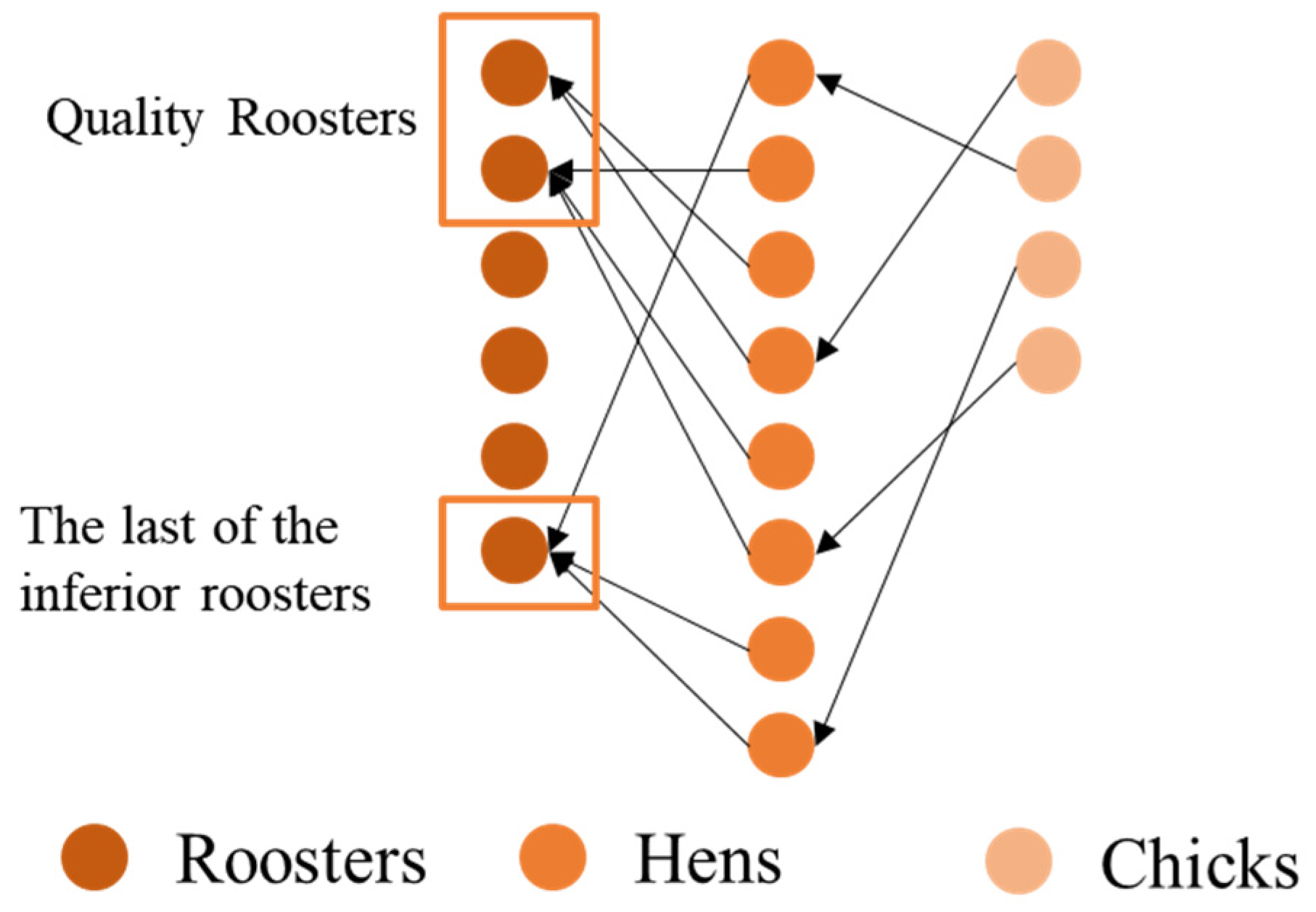
Hens constitute the majority of the swarm. Led by the rooster, the hens perform a local search near the rooster and, thus, the merit of the rooster determines the merit of the hen’s search space. In the original algorithm, the rooster followed by the hen is randomly selected from the whole rooster swarm, and although this approach can improve the diversity of solutions, it limits solution accuracy. Thus, a dynamic constraint is proposed for the roosters, which is given to the high-quality roosters by randomly selecting them from all the roosters, while an inferior rooster is added to the high-quality roosters to ensure the diversity of solutions. As the number of followed roosters gradually decreases, the number of follower hens per rooster gradually increases, which in turn improves the search accuracy in the region around the current rooster. Figure 2 shows the concept of the constraint strategy for hen-following roosters.
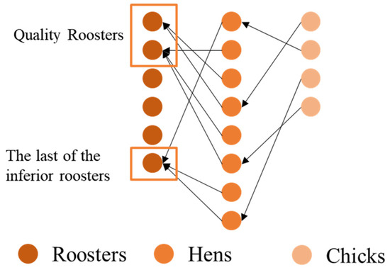
Figure 2.
Rooster-binding following strategies.
The constraint mechanism for hens following the roosters should have the following characteristics:
- (1)
- The total number of roosters is constant, and the number of roosters followed by hens as they transition from following all roosters to following high-quality roosters drops;
- (2)
- In the early iterations, the number of followed roosters should be quickly reduced to determine the approximate range of the optimal solution;
- (3)
- In the late iterations, the variation is kept constant or reduced to achieve a precise search and improve the accuracy of the solution;
- (4)
- There is always a worst rooster among good roosters, which improves the diversity of solutions and helps to avoid falling into local optima.
Based on the above analysis, the constraint equation for hens following the rooster is as follows:
where is the total number of roosters, and is the bound roosters.
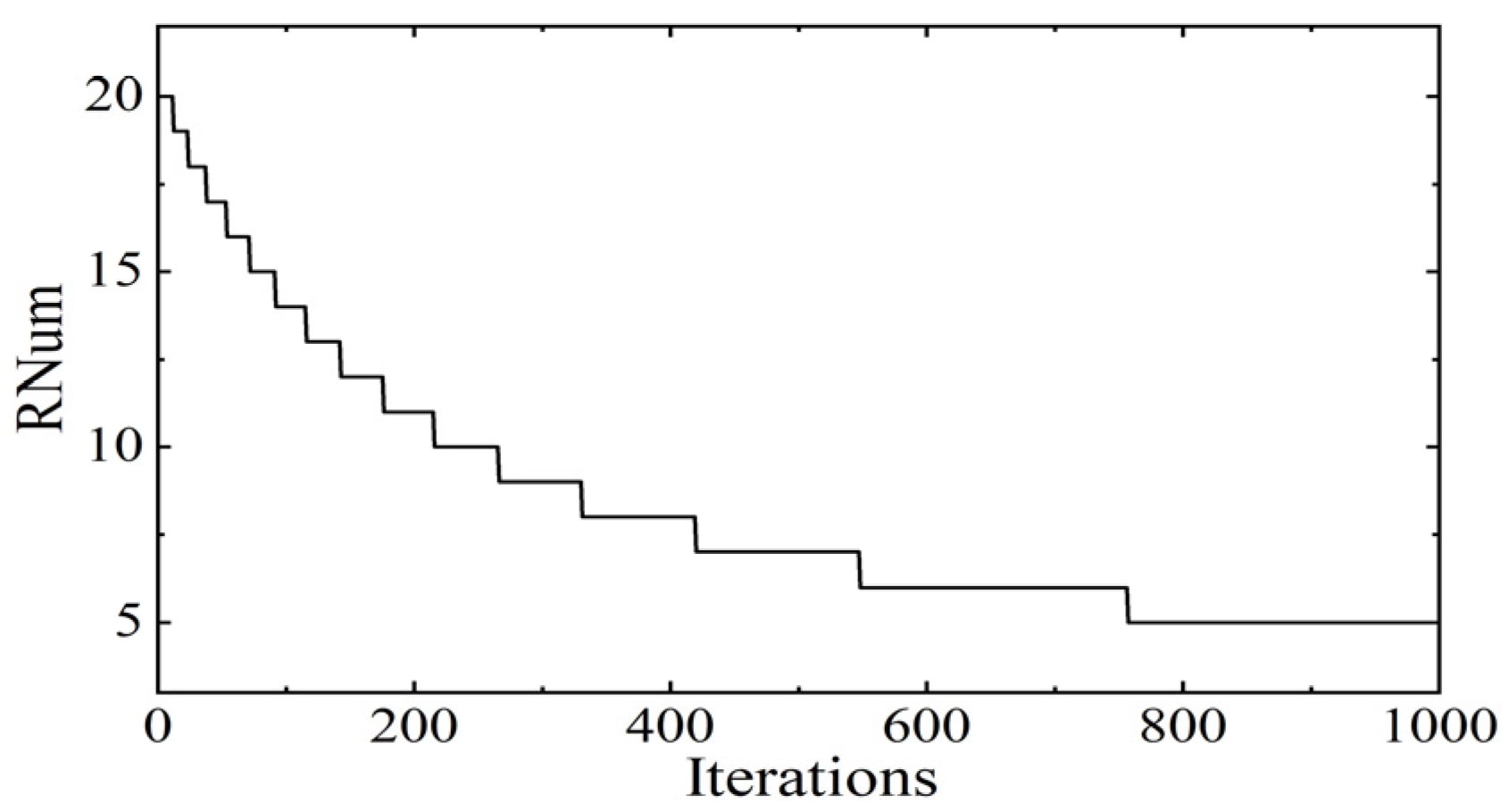
The curve for the change in the number of constrained roosters is shown in Figure 3, where the maximum number of iterations , and the total number of roosters . It can be seen that the number of constrained roosters abruptly decreases in the first 500 iterations and changes relatively little in the last 500 iterations. The above requirements are met.
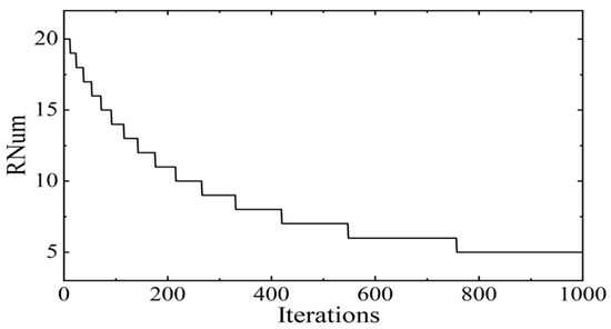
Figure 3.
Constrained rooster number curve.
With the introduction of the highest-value rooster into the hen’s update position, the hen is attracted to this rooster while following the target rooster in the group in which it is located. This ensures that it does not just search randomly around the target rooster in the group, providing it with a certain target that can improve the convergence accuracy to some extent. The concept of the hen’s update strategy following the introduction of the best-quality rooster is shown in Figure 4.
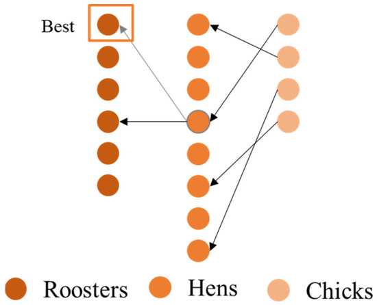
Figure 4.
Double rooster-following strategy.
The equation for the double rooster-following strategy is as follows:
where is the optimal value of the rooster.
2.2. Implementation Steps of the Algorithm
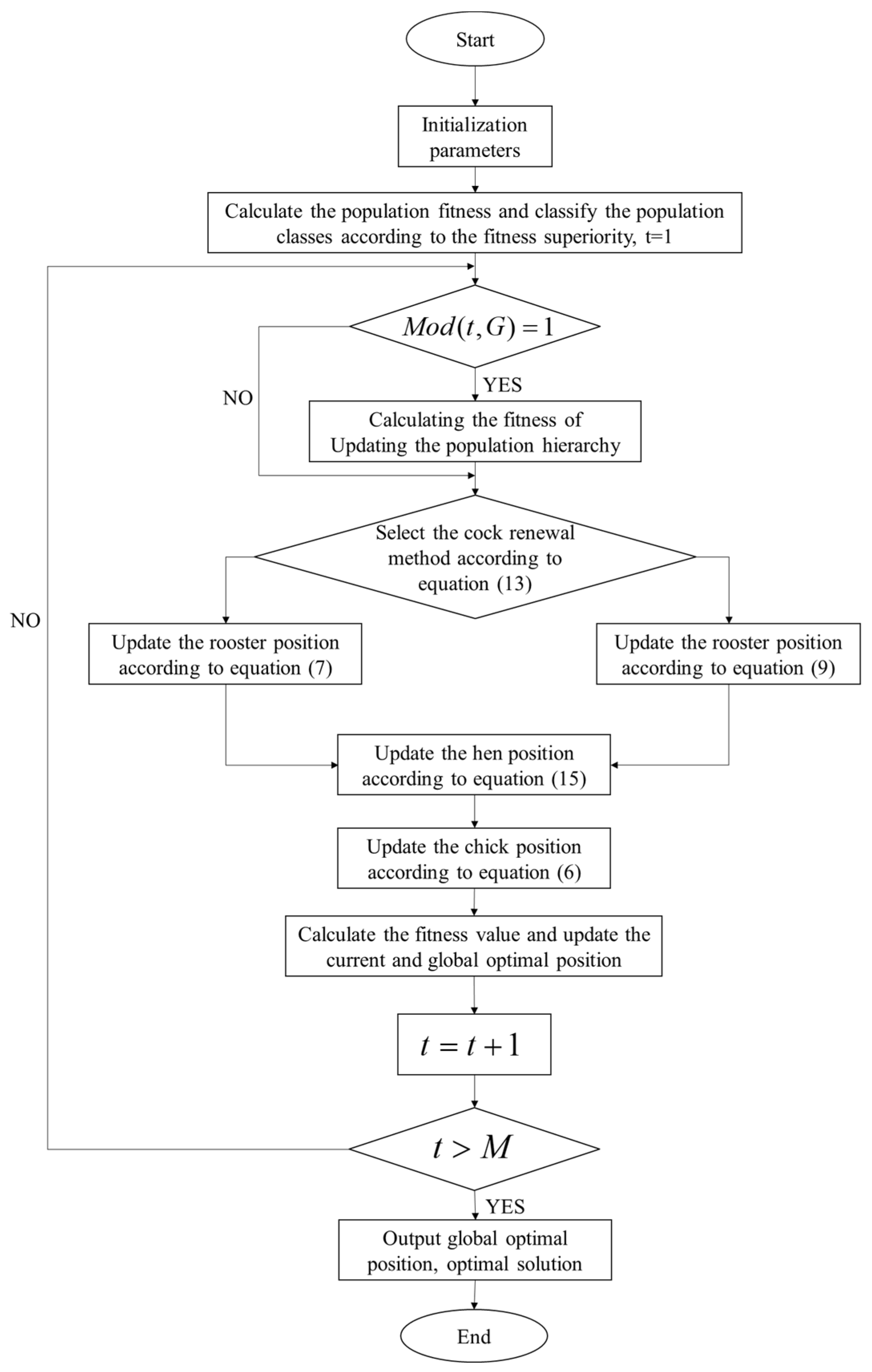
The CSO becomes a PDCSO after simultaneously introducing the parallel policy based on the X-best bootstrap mechanism and the Levy flight rooster update mechanism with a dynamically constrained hen-following target mechanism. The relevant flowchart is shown in Figure 5, and its pseudocode is shown in Algorithm 1.
| Algorithm 1: Pseudocode for the PDCSO algorithm. |
| Initialize a population of N chickens and define the related parameters; Evaluate the chickens’ fitness values, While If Rank the chickens’ fitness values and establish a hierarchal order in the swarm Divide the swarm into different groups and determine the relationship between the chicks and mother hens in a group End For If Select rooster update method using Equation (13) Update its solution/location using Equation (7) or Equation (9) End If Update its solution/location using Equation (15) End If Update its solution/location using Equation (6) End Evaluate the new solution If the new solution is better than the previous one, update it End End |
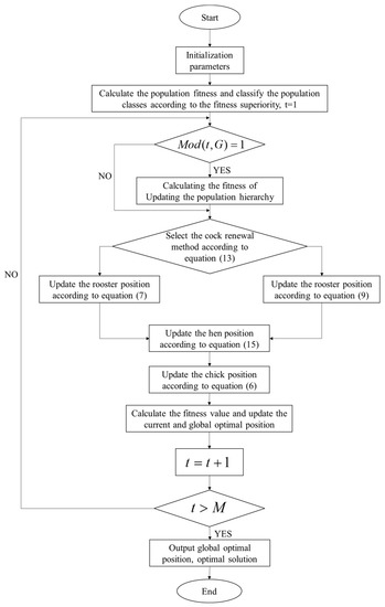
Figure 5.
The flowchart for PDCSO.
2.3. Improved Algorithm Performance Testing
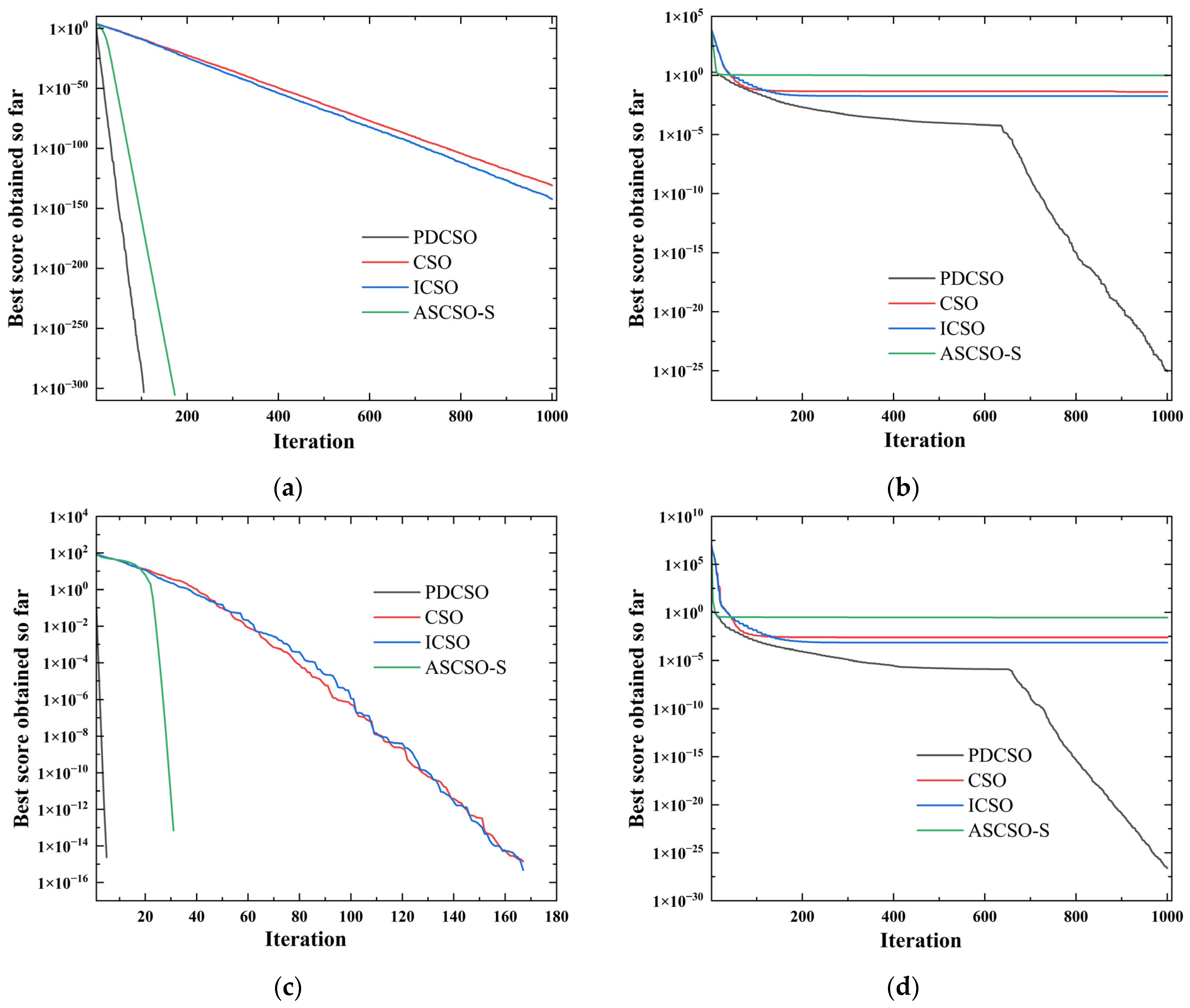
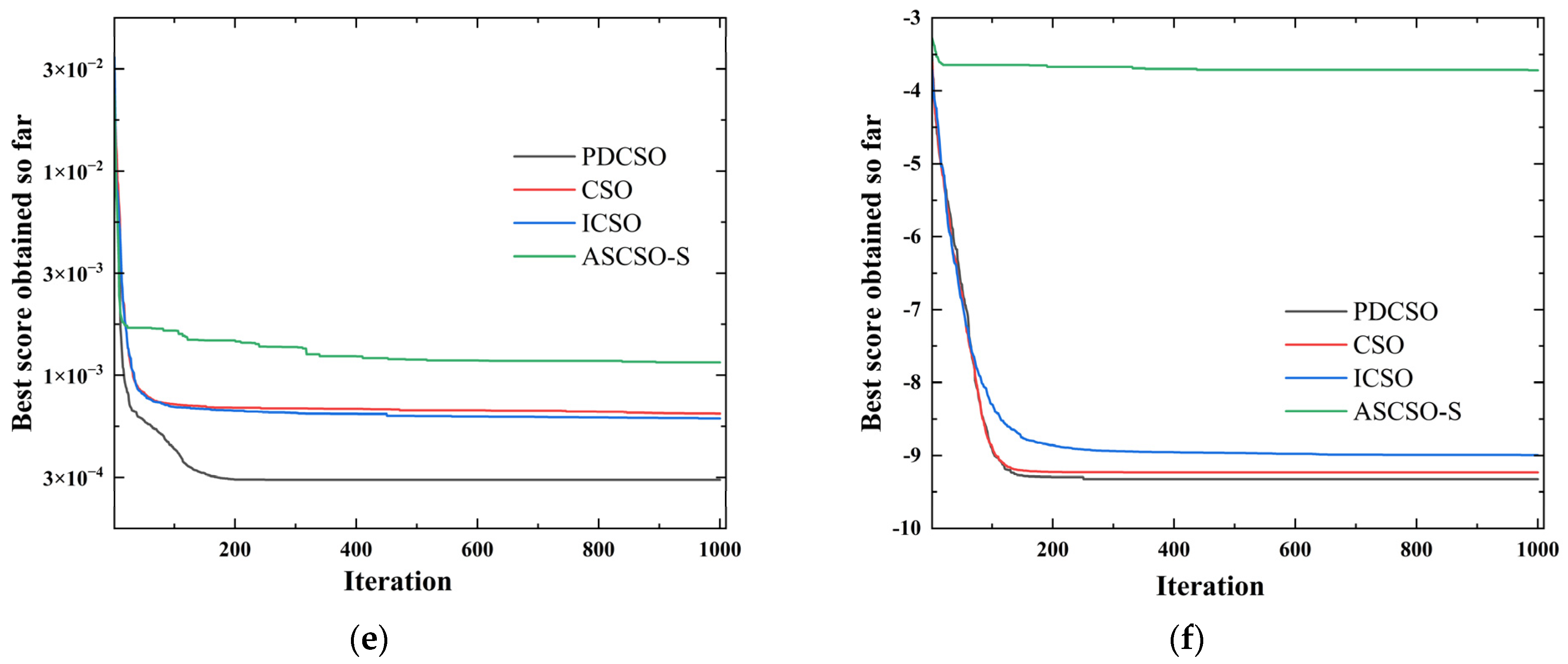
To verify the effectiveness of the proposed improvement mechanism with PDCSO, the improved algorithm was tested with 18 test functions. The simulation environment was MATLAB, and the simulation computer was configured with an Intel® Core™ i7-6700HQ CPU with 2.60 Hz and 16 GB RAM. The information about the test function is shown in Table 1, illustrating the test function’s search range, test dimension and theoretical optimal value. The adjustable dimensionality test functions can be used to test the performance of the algorithm with high dimensionality, and is a fixed-dimension test function. The main algorithms CSO, PDCSO, ICSO [18] and ASCSO-S [17] were compared in the tests. The parameter settings for each algorithm are shown in Table 2. The maximum number of iterations for each algorithm was 1000, and the test results after 30 independent runs are shown in Table 3. Figure 6 shows a partial iterative curve.

Table 1.
Test functions and parameters.

Table 2.
Algorithm parameters.

Table 3.
Test results for different improved algorithms.
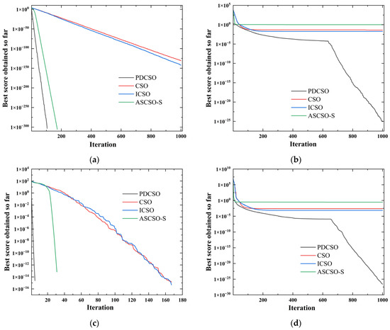
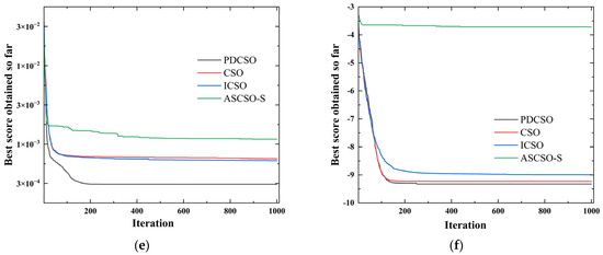
Figure 6.
Partial function convergence curve: (a) function F1; (b) function F5; (c) function F7; (d) function F10; (e) function F13; (f) function F17.
The results in Table 3 and Figure 6 show that the performance of the PDCSO algorithm was much better than that of the other algorithms in terms of optimization accuracy, convergence speed and stability. Compared with ASCSO-S, PDCSO had the same search accuracy, and its parallel strategy could avoid the situation of falling into local optima that resulted from the overreliance of ASCSO-S on X-best bootstrapping. PDCSO could also jump out of local optima in some function tests. In summary, PDCSO outperformed CSO, ICSO and ASCSO-S, which reflects the superiority of PDCSO.
3. Construction of the Optimization Objective Function
3.1. Description of Optimal Time-Shock Planning Problem
By discretizing the motion trajectory to be executed by the robot arm in a Cartesian space, a sequence of spatial positional matrices can be obtained, and the spatial positional sequence can be converted into a sequence of robot-arm joint positions using inverse kinematics. denotes the number of joints in the robot arm, and denotes the time node . The joint position–time node sequence is:
The joint trajectory profile can be obtained by interpolating the above joint position–time node sequence with polynomial or spline functions. The former improves the execution efficiency of the arm, and the latter ensures that shocks are minimized during the execution of the motion trajectory, optimizing two conflicting kinematic performance metrics. The less that joint shocks and drive torque fluctuations occur, the smoother the arm motion.
In this regard, by constructing trajectory profiles for each joint of the robot arm using a five-order B-spline function and by using both joint motion time and shocks as optimization metrics, the optimal time–shock planning problem for the robot arm can be generalized as a multi-objective optimization problem as follows:
Considering the motion constraint for the robot arm, the following constraint is defined:
The weight method is also used to convert the multi-objective optimization problem into a single-objective optimization problem, and the penalty function method is used to convert the constrained problem into an unconstrained problem.
To satisfy the requirements for the continuous jerk trajectory, each joint trajectory third-order curve must be at least geometrically continuous, and since the th order B-spline curve has the property of continuity, it is required that . Therefore, the interpolated curve is constructed using the five-order B-spline function.
3.2. B-Spline Interpolation Trajectory Construction
The order B-spline curve is defined as:
where is the vertex of the characteristic polygon; is known as the th order ( order) basis function; and is the normalized time vector .
The expression of the basis function is derived from the deBoor–Cox recurrence equation.
where is the number of B-sample functions, and is the sequence number of B-sample functions, which specifies that .
In order to make each joint trajectory pass through position nodes in , the control points of the B-sample trajectory equation need to be inverted, and the node values of the B-sample curve located in the node interval are substituted into Equation (21) to obtain , which meets the constraint conditions equation.
Therefore, to add conditions, this study assumes that to obtain the remaining boundary conditions via their configuration.
where are the joint beginning and end velocity and beginning and end acceleration, respectively.
The trajectory curve of joint on is derived from the solved control-vertex and time-node vectors.
4. Simulation and Experimentation
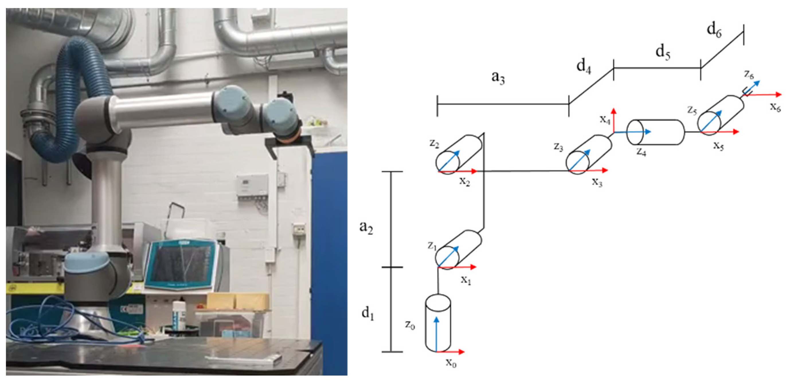
The UR5E robotic arm was used as a simulation test object. A schematic diagram of the UR5E robotic arm body and linkage coordinate system, the D-H parameter table for the UR5E robot arm and the sequence of passed joint positions are shown in Figure 7 and Table 4 and Table 5, respectively.

Figure 7.
UR5E robot and its linkage coordinate system.

Table 4.
Robotic arm D-H parameters.

Table 5.
Sequence of the positions of each joint of the robot arm.
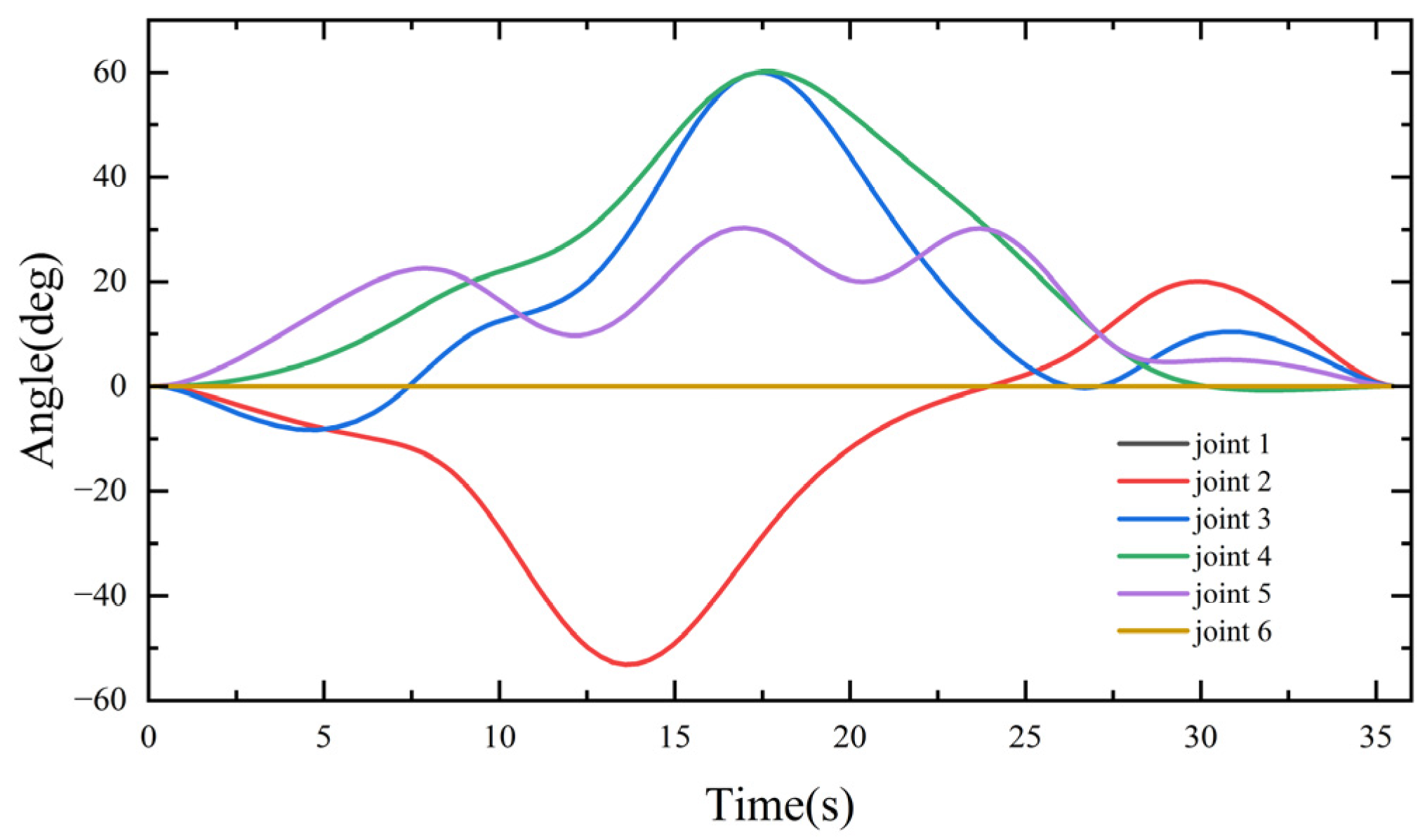
A five-order B-sample was used as the interpolation curve, the start–stop speeds of all joints were set and the acceleration was set as 0. Trajectory optimization simulation was performed with the standard CSO and the PDCSO algorithms, and the parameters for both the CSO and PDCSO algorithms were . Iterative results in Figure 8 were obtained, and the position curves for each joint are shown in Figure 9.
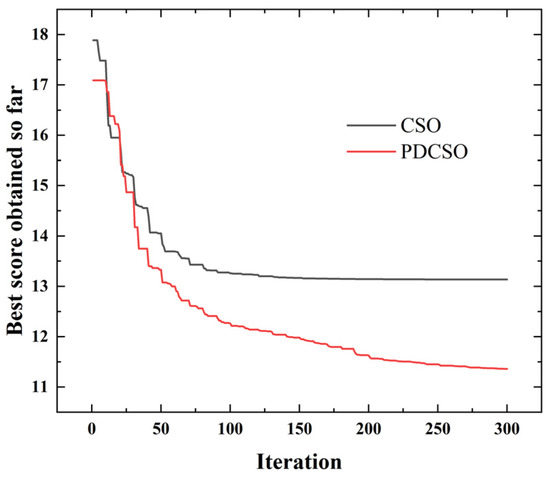
Figure 8.
Comparison of iterative convergence.

Figure 9.
Six joint-angle curves.
4.1. ADAMS Simulation
The kinematics simulation analysis of the robot was run on the platform ADAMS. The driving of each joint was carried out in this dynamic simulation, and the torque change curve for each joint was obtained. In this study, there was no position change between joint one and joint six; therefore, only the other four joints were considered, and the torque change comparison curve is shown in Figure 10.


Figure 10.
Comparison of joint torque curves: (a) joint two; (b) joint three; (c) joint four; (d) joint five.
4.2. Experiment
The UR5E robotic arm test platform was set up as shown in Figure 11. The motion control commands were written on the host computer and passed to the robotic arm controller via Modbus-TCP. Then, the robotic arm controller converted the commands into electrical signals for the robotic arm body to finally realize the movement of the robotic arm according to the given time–displacement curve. In the upper computer, the robot arm 30003 interface signal was read by the script command to obtain the real-time joint torque of the robot arm. A comparison of the torque curves for each joint before and after optimization is shown in Figure 12.

Figure 11.
UR5E robotic arm test platform.


Figure 12.
Experimental comparison of joint torque curves: (a) joint two; (b) joint three; (c) joint four; (d) joint five.
As shown in Figure 8, DRCSO had higher search accuracy than CSO and could jump out of the optimal local solution. The ADAMS simulation showed that the moment continuously and smoothly changed throughout the motion of the robot, and there were no collisions in the robot arm body; therefore, it was stable and safe for a real machine test. Since the simulation process was in an ideal state, only the influence of weight was considered. The characteristics of the friction between the joints of the robot arm were not considered, and there were discrepancies between the modeling and the actual results. Therefore, the actual results were not exactly the same as the simulation results, but the trends for the whole torque were similar and showed smooth and stable characteristics. The reliability of the five-order B-spline function interpolation was proven. The running time was greatly reduced by the PDCSO algorithm, from 45 s before to 35.3 s after optimization (a reduction of 21.11%). The torque peak was smaller, the torque change was smoother and the unnecessary torque change was reduced. The torque change rates for joints two to five were reduced by 8.81%, 6.71%, 2.74% and 11.70%, respectively. The experiments made it clear that the optimized robot arm ran fast and smoother.
5. Conclusions
In order to solve the problems of low solution accuracy and slow convergence speed with the basic CSO algorithm in a time-jerk optimization task for a robotic arm, we used the proposed PDCSO algorithm and a rooster update mechanism based on a parallel strategy involving X-best guidance and Levy flight and a dynamically constrained hen-following target mechanism, which improved the accuracy of the algorithm and helped to avoid local optima. The optimization simulation results for 18 test functions showed that the proposed PDCSO algorithm exhibited significant improvement in terms of the search accuracy, convergence speed and stability of the algorithm compared to the basic CSO algorithm and its other improved versions.
The results from the ADAMS simulations and real machine experiments showed that the trajectory obtained by the PDCSO optimization method satisfied various kinematic constraints on the cumulative effect of execution time and shocks. The accumulation of motion shocks was reduced by 8.81%, 6.71%, 2.74% and 11.70%, so the joint motion was more stable.
Author Contributions
Conceptualization, Y.L. (Yankun Li), Y.L. (Yuyang Lu), M.Z., X.G. and Y.L. (Yu Liu); Methodology, Y.L. (Yankun Li), Y.L. (Yuyang Lu), M.Z., X.G. and Y.L. (Yu Liu); Software, Y.L. (Yankun Li), Y.L. (Yuyang Lu), C.X. and X.G.; Validation, Y.L. (Yankun Li), Y.L. (Yuyang Lu) and D.L.; Formal analysis, Y.L. (Yankun Li), Y.L. (Yuyang Lu), D.L., C.X., X.G. and Y.L. (Yu Liu); Investigation, Y.L. (Yankun Li), Y.L. (Yuyang Lu), D.L. and Y.L. (Yu Liu); Resources, C.X.; Writing—original draft, Y.L. (Yankun Li) and Y.L. (Yu Liu); Writing—review & editing, Y.L. (Yankun Li), Y.L. (Yuyang Lu), D.L., M.Z., X.G. and Y.L. (Yu Liu); Visualization, M.Z.; Supervision, M.Z., X.G. and Y.L. (Yu Liu); Project administration, Y.L. (Yuyang Lu); Funding acquisition, M.Z. and Y.L. (Yu Liu). All authors have read and agreed to the published version of the manuscript.
Funding
This research was funded by the National Natural Science Foundation of China (grant no. 51875253), the Ministry of Education Humanities and Social Sciences Research Planning Fund Project (19YJAZH123) and Jiangsu Provincial Key Research and Development Program (BE2022069-2).
Institutional Review Board Statement
Not applicable.
Informed Consent Statement
Not applicable.
Data Availability Statement
Not applicable.
Conflicts of Interest
The authors declare no conflict of interest.
References
- Abu-Dakka, F.J.; Rubio, F.; Valero, F.; Mata, V. Evolutionary indirect approach to solving trayectory planning problem for industrial robots. Eur. J. Mech. 2013, 42, 210–218. [Google Scholar] [CrossRef]
- Cui, L.; Wang, H.; Chen, W. Trajectory planning of a spatial flexible manipulator for vibration suppression. Robot. Auton. Syst. 2019, 123, 103316. [Google Scholar] [CrossRef]
- Tang, L.; Gosselin, C.; Tang, X.; Jiang, X. Dynamic trajectory planning of planar two-dof redundantly actuated cable-suspended parallel robots. In Proceedings of the 2014 IEEE/RSJ International Conference on Intelligent Robots and Systems, Chicago, IL, USA, 14–18 September 2014. [Google Scholar]
- Wang, Y.L.; Yuan, R.B.; Yuan, A.H. Application of differential particle swarm algorithm in inverse kinematics solution of puma robot. Softw. Guide 2020, 19, 203–207. [Google Scholar] [CrossRef]
- Li, L.; Shang, J.Y.; Feng, Y.L.; Huai, Y.W. A review of research on trajectory planning of articulated industrial robots. Comput. Eng. Appl. 2018, 54, 36–50. [Google Scholar] [CrossRef]
- Peng, X.; Chen, G.; Tang, Y.; Miao, C.; Li, Y. Trajectory optimization of an electro-hydraulic robot. J. Mech. Sci. Technol. 2020, 34, 4281–4294. [Google Scholar] [CrossRef]
- Huang, J.; Hu, P.; Wu, K.; Zeng, M. Optimal time-jerk trajectory planning for industrial robots. Mech. Mach. Theory 2018, 121, 530–544. [Google Scholar] [CrossRef]
- Zhang, Y.; Sun, Z.; Sun, Q.; Wang, Y.; Yang, J. Time-jerk optimal trajectory planning of hydraulic robotic excavator. Adv. Mech. Eng. 2021, 13, 1014. [Google Scholar] [CrossRef]
- Du, Y.; Chen, Y. Time Optimal Trajectory Planning Algorithm for Robotic Manipulator Based on Locally Chaotic Particle Swarm Optimization. Chin. J. Electron. 2022, 31, 906–914. [Google Scholar]
- Choi, Y.; Kim, D.; Hwang, S.; Kim, H.; Kim, N.; Han, C. Dual-arm robot motion planning for collision avoidance using B-spline curve. Int. J. Precis. Eng. Manuf. 2017, 18, 835–843. [Google Scholar] [CrossRef]
- Long, Z.; Li, X.T.; Shuai, T.; Wen, F.J.; Feng, W.R.; Liang, C.P. A review of the current status of industrial robot trajectory planning research. Mech. Sci. Technol. 2021, 40, 853–862. [Google Scholar] [CrossRef]
- Meng, X.B.; Gao, X.Z.; Lu, L.; Liu, Y.; Zhang, H. A new bio-inspired optimisation algorithm: Bird Swarm Algorithm. J. Exp. Theor. Artif. Intell. 2015, 28, 673–687. [Google Scholar] [CrossRef]
- Deb, S.; Gao, X.Z.; Tammi, K.; Kalita, K.; Mahanta, P. Recent Studies on Chicken Swarm Optimization algorithm: A review (2014–2018). Artif. Intell. Rev. 2020, 53, 1737–1765. [Google Scholar] [CrossRef]
- Irsalinda, N.; Thobirin, A.; Wijayanti, D.E. Chicken Swarm as a Multi Step Algorithm for Global Optimization. Int. J. Eng. Sci. Invent. 2017, 6, 8–14. [Google Scholar]
- Zhang, M.X.; Zhang, D.M.; Yang, J.Q.; Zhu, C. An improved chicken swarm algorithm based on forward learning and backward learning. Microelectron. Comput. 2018, 35, 6. [Google Scholar]
- Zhang, K.W.; Zhao, X.L.; He, L.; Li, Z.Z. A chicken swarm algorithm with improved x-best guided individuals and dynamic rank update mechanism. J. Beijing Univ. Aeronaut. Astronaut. 2021, 47, 15. [Google Scholar]
- Haiyan, L.U.; Xiang, L.; Shen, W.; Yanchun, G.U. Adaptive Simplified Chicken Swarm Optimization Based on Inverted S-Shaped Inertia Weight. Chin. J. Electron. 2022, 31, 367–386. [Google Scholar]
- Liang, X.; Kou, D.; Wen, L. An improved chicken swarm optimization algorithm and its application in robot path planning. IEEE Access 2022, 8, 49543–49550. [Google Scholar] [CrossRef]
- Huang, X.; Ye, C.M.; Zheng, J. Hybrid improved search strategy for chicken swarm optimization algorithm. Comput. Eng. Appl. 2018, 54, 176–181. [Google Scholar] [CrossRef]
- Kamaruzaman, A.F.; Zain, A.M.; Yusuf, S.M.; Udin, A. Levy Flight Algorithm for Optimization Problems - A Literature Review. Appl. Mech. Mater. 2013, 421, 496–501. [Google Scholar] [CrossRef]
Disclaimer/Publisher’s Note: The statements, opinions and data contained in all publications are solely those of the individual author(s) and contributor(s) and not of MDPI and/or the editor(s). MDPI and/or the editor(s) disclaim responsibility for any injury to people or property resulting from any ideas, methods, instructions or products referred to in the content. |
© 2023 by the authors. Licensee MDPI, Basel, Switzerland. This article is an open access article distributed under the terms and conditions of the Creative Commons Attribution (CC BY) license (https://creativecommons.org/licenses/by/4.0/).


