Short-Term Power Load Forecasting Based on an EPT-VMD-TCN-TPA Model

Abstract

Accurate short-term load forecasting is the key to ensuring smooth and efficient power system operation and power market dispatch planning. However, the nonlinear, non-stationary, and time series nature of load sequences makes load forecasting difficult. To address these problems, this paper proposes a short-term load forecasting method (EPT-VMD-TCN-TPA) based on the hybrid decomposition of load sequences, which combines ensemble patch transform (EPT), variational modal decomposition (VMD), a temporal convolutional network (TCN), and a temporal pattern attention mechanism (TPA). In which, the trend component (Tr(t)) and the residual fluctuation component (Re(t)) of the load series are extracted using EPT, and then the Re(t) component is decomposed into intrinsic modal function components (IMFs) of different frequencies using VMD. The Tr(t) and IMFs components of the fused meteorological data are predicted separately by the TCN-TPA prediction model, and finally, the prediction results of each component are reconstructed and superimposed to obtain the final predicted value of the load. In addition, experiments after reconstructing each IMF component according to the fuzzy entropy (FE) values are discussed in this paper. To evaluate the performance of the proposed method in this paper, we used datasets from two Areas of the 9th Mathematical Modeling Contest in China. The experimental results show that the predictive precision of the EPT-VMD-TCN-TPA model outperforms other comparative models. More specifically, the experimental results of the EPT-VMD-TCN-TPA method had a MAPE of 1.25% and 1.58% on Area 1 and Area 2 test sets, respectively.

1. Introduction

As countries and regions around the world rely more and more on electricity, this requires a higher level of security, reliability, and economy in the supply of electricity [1]. For example, China’s green development goals of “carbon peaking” and “carbon neutrality” also make electricity play an important role in the national economy [2]. With the advancement of technology, the storage, generation, transmission, distribution, and consumption of electrical energy is no longer an isolated process; therefore, in the traditional power system, effective measures must be taken to maintain the dynamic balance of electrical energy supply and demand [3]. The use of accurate power load forecasting not only provides a reference for the dynamic balance between power supply and demand, but also facilitates power plants to reasonably dispatch power generation, schedule the start and stop of generating units, improve the utilization rate of power generation equipment, and reduce the cost of power generation [4]. Therefore, accurate load forecasting is of great importance to the development of power systems.

According to the length of the forecast period, power load forecasting can be divided into four types: ultra-short-term load forecasting, short-term load forecasting, medium-term load forecasting, and long-term load forecasting [5]. Different cycles of load forecasting have different roles and meanings, among which online control and real-time monitoring of power systems rely on ultra-short-term load forecasting. Short-term load forecasting can coordinate the daily start/stop and generation plans of each generating unit, while medium- and long-term load forecasting aims to provide a reference basis for the long-term planning of power systems, etc. [6]. In previous studies, numerous scholars have proposed many methods to improve the accuracy of load forecasting, most of which focus on methods for short-term load forecasting. These methods are divided into three main categories based on statistical models, artificial intelligence prediction models, and combined prediction models, as shown in Figure 1. Multiple linear regression (MLR) [7], exponential smoothing (ES) [8], Kalman filter [9], the Hidden Markov model (HMM) [10], and the Autoregressive Integrated Moving Average Model (ARIMA) [11] are commonly used in statistical models for load forecasting. In Ref. [8], Christiaanse et al. developed a forecasting model with high accuracy and simple operation based on the exponential smoothing method and analyzed the role of exponential smoothing in load forecasting. In Ref. [11], Wu et al. proposed an autoregressive differential moving average model based on long-term dependence and combined it with the cuckoo search algorithm to optimize the parameters of the prediction model. The experimental results show that the ARIMA model has good prediction results in short-term load forecasting. In Ref. [12], Duan L et al. considered the external factors and the power system itself in medium- and long-term load forecasting and used a multilevel recursive regression method for medium- and long-term load forecasting to improve the forecasting accuracy by accurately predicting the important functions of time-varying parameters and related factors. Although statistical model-based methods have the characteristics of relatively simple models and fast prediction, these models usually target linear relational models, which require high smoothness of existing data, and non-linear relationships are more difficult to be captured accurately. Due to the combination of multiple factors, the variation of the load series has high uncertainty and complexity, which makes the traditional statistical model prediction unsatisfactory. In recent years, with the improvement of computer performance, the forecasting methods of artificial intelligence models have been applied to nonlinear time series load forecasting problems.

Short-term load forecasting methods based on artificial intelligence mainly include machine learning and deep learning models. Through machine learning techniques, we can learn and mine the non-linear relationship between the independent and dependent variables, and build regression models to predict short-term loads. Some common algorithms, such as support vector regression (SVR) [13], back propagation neuron networks (BPNNs) [14], and artificial neural networks (ANNs) [15], have been widely used for load forecasting. In Ref. [13], the authors implemented a generic short-term load forecasting strategy based on support vector machines by improving the generation process in the SVR input model and selecting the hyperparameters of the SVR model based on a particle swarm optimization algorithm, which was tested on two publicly available datasets to verify its effectiveness. In Ref. [14], the authors proposed a short-term load forecasting method based on a hybrid optimization algorithm and a BPNN for the load forecasting of paper enterprises, and the experimental results showed that the forecasting results of the forecasting model using the hybrid optimization algorithm outperformed the forecasting results of the single model. Although machine learning methods can handle nonlinear data well, these methods cannot effectively extract data features of load sequences due to the complexity and time series nature of load data. As deep learning continues to evolve, it becomes the focal point of load forecasting. In recent years, convolutional neural networks (CNNs), deep belief networks (DBNs), and deep neural networks (DNNs) have achieved remarkable results in the field of short-term load forecasting [16,17,18]. Although these methods are effective in extracting features of multidimensional load data and thus improving prediction precision, they cannot capture the time series features of load sequences when used alone. A recurrent neural network (RNN) is a neural network based on gate structure control, which is able to adjust the information based on past timestamps and current input values, overcoming the problem that ANN models do not handle temporal load data well [19]. A RNN can adversely affect prediction accuracy when dealing with complex nonlinear data due to the possibility of gradient explosion and gradient disappearance, thus limiting its application. The long short-term memory (LSTM) [20] network is an improved version of the RNN, which effectively solves the problem of gradient disappearance and gradient explosion that may occur when the RNN processes complex data by providing memory function and gate structure. The model has been widely used for short-term load forecasting [21,22]. Weicong Kong et al. conducted experiments using a framework based on an LSTM recurrent neural network on a real dataset and finally achieved better prediction results [23]. However, it is difficult to select parameters for the LSTM network as the training data increases. In Ref. [24], the authors first preprocess the load data and predict the load through the established gated recursive unit (GRU) network. The GRU greatly reduces the number of network parameters by merging the forgetting and input gates of the LSTM, which greatly improves the performance of the neural network and makes it easier to achieve convergence. Considering that the LSTM and GRU can only encode the information of load sequences from front to back and cannot adequately consider the future information, some scholars have used bidirectional long short-term memory (BiLSTM) and bidirectional gated recurrent unit (BiGRU) for load prediction [25,26]. In Ref. [25], the authors design a BiLSTM forecasting model based on improved particle swarm optimization, which designs a selection mechanism taking into account trend similarity and momentary similarity, thus combining the predicted and historical similar values and improving the forecast precision. In Ref. [26], the authors proposed a CNN-BiGRU method for short-term load prediction in which high-dimensional features and time-dependent features of the load data were extracted using a CNN and BiGRU, respectively, and an attention mechanism was introduced to the BiGRU network, and the results showed that the method would be more effective than the LSTM method. The BiLSTM and BiGRU networks have both forward and backward sequential information inputs, which can fully extract information from the load data and thus may improve the accuracy of feature extraction to some extent. In order to solve the problems of CNN’s inability to capture sequence timing features and the lack of using convolutional operations to extract data features in recurrent neural networks, temporal convolutional networks (TCNs) were created. The TCN is a new architecture based on convolutional neural networks that can efficiently extract sequence timing features. The TCN has improved on the basis of the CNN for the time series problem and is able to extract feature information of nonlinear time series data, while the TCN model solves the problem of gradient explosion and gradient disappearance by initializing the weight parameters. For load prediction as a complex nonlinear optimization problem, Song et al. built a thermal load prediction model based on TCN networks to achieve the extraction of complex data features and accurate load prediction [27]. Due to the advantages of TCN networks, many scholars have used them for short-term load forecasting [28,29].

Considering the non-linear and fluctuating characteristics of power load data, many experts and scholars pre-process the power load data before forecasting. One approach is to use a suitable method to classify the time series data into deterministic and stochastic components, and then model them separately based on these two different types of components. The deterministic component takes into account the characteristics of the load series such as trend, annual, quarterly, and weekly cycles, and date similarity, while other stochastic influences will determine the stochastic component. In Ref. [30], Ismail Shah et al., considering the characteristics such as polar values of electric load data, proposed a function data modeling method that divides the sequence after polar value processing, into deterministic and random components, and uses generalized additive modeling techniques to model the deterministic component and three different models to model the random component. The experimental results show that the prediction error based on the deterministic component and the stochastic component is predicted separately with lower prediction errors than the classical comparison models. Meanwhile, in Ref. [31], Ismail Shah et al. first divided the time series (demand and price) into deterministic and stochastic components. The deterministic component is modeled using parametric and nonparametric methods, and the stochastic component is modeled using univariate autoregression (AR) and multivariate vector autoregression (VAR), and finally, the model proposed in the paper is known to have better forecasting ability by evaluating the indicators, and the effectiveness of the model proposed in the paper is further verified by statistical significance. In Ref. [32], the method based on component estimation also achieved better prediction results. Another approach is to use signal decomposition methods to decompose the load data sequence into several relatively smooth sequences, and then predict each component separately. These signal decomposition methods are mainly wavelet transforms, empirical modal decomposition (EMD), and improved methods based on EMD, etc. In Ref. [33], the authors propose a prediction method based on a combination of wavelet decomposition and second-order gray neural networks. In Ref. [34], the authors first decompose the load sequence using EMD, followed by modeling prediction using a BiLSTM network based on an attention mechanism. In Ref. [35], the authors first decompose the load sequences using an ensemble empirical modal decomposition (EEMD), followed by reconstructing enough new sequences based on the approximate entropy of each component, and finally use an extreme learning machine (ELM) to predict each sequence separately and superimpose their results. Although these decomposition methods make load forecasting more accurate to a certain extent, they also have certain problems. For example, the effect of wavelet transformation is related to the choice of wavelet basis, which is less applicable. EMD decomposition tends to lead to modal confusion and endpoint effects when there are significant step changes in the signal. The EEMD decomposition reduces the residual auxiliary noise and reconstruction errors during EMD decomposition by adding Gaussian white noise several times, thus reducing the generation of modal aliasing. In recent years, variational modal decomposition (VMD) has been widely used in the field of short-term power load forecasting [36,37]. With the VMD decomposition technique, Cai et al. divided the load sequence into more stable parts and used a predictive network model to make accurate predictions for these parts [38]. The experimental results show that the VMD decomposition technique can significantly improve the accuracy and precision of load prediction. VMD is fundamentally different from EMD in that it uses a non-recursive approach to achieve signal decomposition and can automatically adjust the number of decompositions according to the actual situation, thus effectively separating the intrinsic modal components and also effectively solving the problems of modal aliasing and endpoint effects. Recently, an ensemble patch transform (EPT) for signal decomposition and filtering has been proposed by Kim et al. [39]. This EPT method can effectively decompose complex signals by specific transformations and can extract features such as trends of non-smooth series. In the short-term load forecasting model proposed in this paper, we use a hybrid decomposition technique based on EPT and VMD to effectively decompose and extract the features of the load sequence.

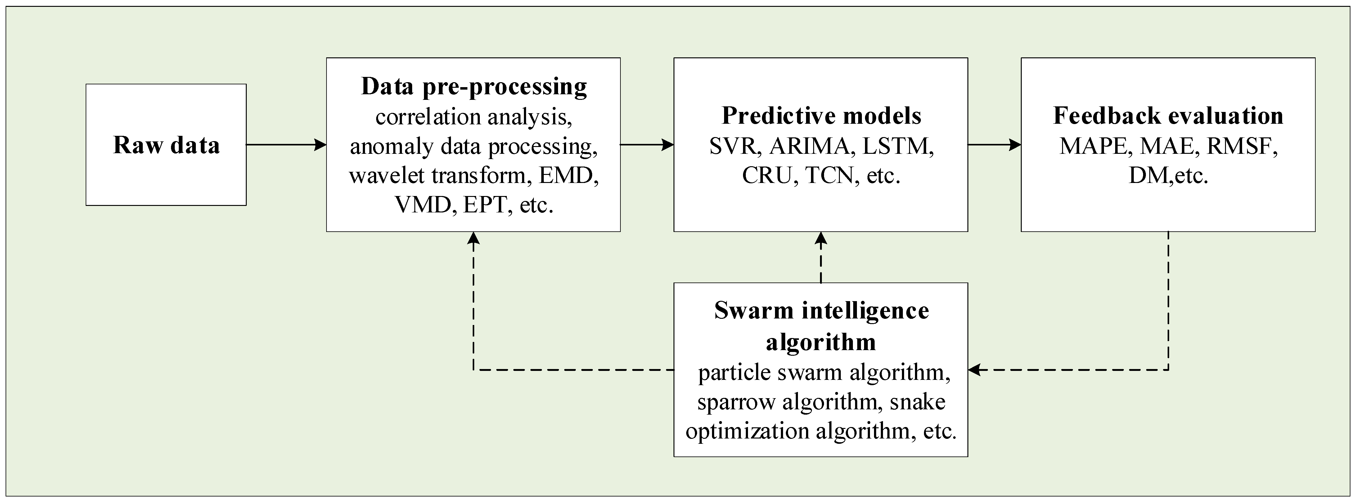
In summary, a combined forecasting model based on optimization algorithms, attention mechanisms, and various forecasting methods can be found throughout, as seen in the general process of electric load forecasting shown in Figure 2. In Ref. [40], the authors used a combined approach of neural networks and particle swarm optimization algorithms to forecast load, which was tested on data from a North American electric utility, and acceptable accuracy was obtained. In Ref. [41], the authors developed a novel multi-dual forecasting system for electricity prices using multivariate and multi-input–multi-output structures. In this model, the data obtained from pre-processing are predicted by a back propagation network, a BiLSTM network, and a GRU network, and finally, the final prediction results are obtained based on the combined strategy of the salp swarm algorithm, and the experimental results show that the proposed method achieves good prediction results. In Ref. [42], the authors propose a hybrid GWO-CNN-BILSTM prediction model for the short-term load prediction of buildings. In this method, a CNN is used to extract features in load sequences, BILSTM can learn both forward and backward data features, and a GWO is used for parameter search optimization of the CNN and BILSTM networks, and finally, four different cases are analyzed to verify the effectiveness of the proposed method. A nice combinatorial model has also been proposed in Ref. [43].

Considering the volatility, nonlinearity, and time series of load series, this paper proposes a short-term load forecasting method based on the combination of EPT-VMD hybrid decomposition and the TCN-TPA network model, called EPT-VMD-TCN-TPA. Compared with other methods, the EPT method used in this paper before using VMD will extract the trend component of the load series, while the VMD method will further reduce the volatility of the remaining fluctuation components. The TCN model based on the temporal attention mechanism used in this paper not only focuses more on the temporal characteristics but also the TCN model is suitable for the prediction of large data volume. First, the trend component (Tr(t)) and the residual fluctuation component (Re(t)) of the load series are extracted using the EPT method. The residual fluctuation component (Re(t)) is then adaptively decomposed into intrinsic modal functions (IMFs) with different central frequencies using the VMD method. Finally, the Tr(t) component, as well as the IMF component, are combined with meteorological influence factors, respectively, and the TCN-TPA network is used to train and predict the electric load. We also discuss the complexity of using fuzzy entropy (FE) to calculate the components of IMFs, and the intrinsic modal function (IMF) components with similar complexity are reorganized into a new component (FE-IMF), which is called the EPT-VMD-FE-TPA-TCN load prediction model. Simulation modeling was conducted using two regional load datasets provided by the 9th National Student Electrician Mathematical Modeling Competition in China, and the results show that the proposed EPT-VMD-TCN-TPA short-term electric load forecasting model predicts better precision than other comparative models and has better applicability.

The main contributions of this paper are further elucidated as follows:

(1)

Since the load series has a certain fundamental trend, the fundamental trend dominates the direction of the load series over time. The established EPT can accurately extract the fundamental trend of the load series, thus improving the accuracy of short-term load forecasting.

(2)

The adopted VMD decomposes the residual fluctuation series into several subseries with different center frequencies, which further reduces the non-smoothness of the fluctuation series. The number of decompositions of the VMD is determined using the ratio of residual energy, which makes the decomposed subsequences smoother.

(3)

The experimental results show that the EPT-VMD hybrid decomposition method proposed in this paper is effective for load prediction.

(4)

The TCN-TPA network is used for the prediction of individual components so that the temporal characteristics of these sequences can be better extracted. The temporal pattern attention mechanism incorporated in the TCN network can better assign different weights to different variables at the same time step compared to the ordinary attention mechanism. The temporal pattern attention mechanism enhances the impact of temporal attributes of multivariate load sequences on load prediction.

(5)

In further experiments, FE was used to analyze the complexity of the IMF components and to reconstruct these components using similar entropy values. The experimental results show that the EPT-VMD-FE-TCN-TPA reconstructed model using FE has higher operational efficiency compared to the EPT-VMD-TCN-TPA prediction model, but the prediction precision is reduced.

The rest of the paper is organized as follows. Section 2 presents the relevant methods. Section 3 explores the proposed model. Section 4 provides an analysis and discussion of the experimental results. Section 5 outlines the experimental results on dataset II. Finally, Section 6 concludes the paper.

2. Related Theories and Methods

This section first introduces two data decomposition methods, ensemble patch transform (EPT) and variational modal decomposition (VMD). Then, a data sequence complexity analysis method, FE, is introduced. finally, the temporal convolutional network (TCN) and temporal pattern attention (TPA) mechanisms are introduced.

2.1. Ensemble Patch Transformation (EPT)

The ensemble patch transformation was proposed by Kim et al. [39]. The EPT method uses the multi-scale concept of computer vision scale space theory to enhance the recognition of local features in the signal data and extract the essential components of the signal data. It consists of two key components, the “patch process” and the “ensemble process”. Due to the flexibility of the EPT framework and the adaptability of the parameters, EPT can be used to discover specific patterns in signal data, such as trends, sudden changes, and periodicity. The text will use EPT to extract the trend component of the load series. Both components will be described below.

2.1.1. Patch Process

A “patch process” is a dependent patch of data at a given time $t$, designed to identify local features of the data. Two types of patches are considered in EPT, rectangular and oval patches. The differences between the two types of patches are not very obvious. Using an oval patch allows us to obtain the central tendency of the data, as the generated curves are smoother. However, there is a need to capture abrupt changes in the data in highly non-smooth load sequences, and in this case, a rectangular patch is more suitable than an oval patch. Therefore, a rectangular patch will be used in this paper for our proposed short-term load prediction model. Only the rectangular patch is described below.

Given a period $\tau$, the patch $P_t^{\tau }(X_t)$ of the load sequence $X_t$ at time $t$ is centered at the point $(t,X_t)$. The patch at this location $(t,X_t)$ is a closed rectangle formed by the points $\left(t+k,{\min }_{k\in \left[-\tau /2,\tau /2\right]}\left\{X_{t+k}\right\}-0.5\gamma \tau \right)$ and $\left(t+k,{\max }_{k\in \left[-\tau /2,\tau /2\right]}\left\{X_{t+k}\right\}+0.5\gamma \tau \right)$, where $k\in \left[-\tau /2,\tau /2\right]$, the width of the patch is $\tau$ and the height is $h_t^{\tau }$.

$$h_t^{\tau }={\max }_{k\in \left[-\tau /2,\tau /2\right]}\left\{X_{t+K}\right\}-{\min }_{k\in \left[-\tau /2,\tau /2\right]}\left\{X_{t+K}\right\}+\lambda \tau$$

(1)

where $\gamma$ is the scale factor.

In order to make the upper and lower envelopes of the extracted load series more homogeneous and thus extract a more stable load trend, the value of $\gamma$ is taken as 1 in this paper.

The upper envelope of the rectangular patch is $U_t^{\tau }\left(X_t\right)$, the lower envelope is $L_t^{\tau }\left(X_t\right)$, and the average envelope is $M_t^{\tau }\left(X_t\right)$:

$$U_t^{\tau }\left(X_t\right)={\max }_{k\in \left[-\tau /2,\tau /2\right]}\left\{X_{t+k}\right\}+0.5\gamma \tau$$

(2)

$$L_t^{\tau }\left(X_t\right)={\max }_{k\in \left[-\tau /2,\tau /2\right]}\left\{X_{t+k}\right\}-0.5\gamma \tau$$

(3)

$$M_t^{\tau }\left(X_t\right)=\frac{1}{2}\left(U_t^{\tau }\left(X_t\right)+L_t^{\tau }\left(X_t\right)\right)$$

(4)

2.1.2. Ensemble Process

The “ensemble process” is an “ensemble” obtained by shifting the time point $t$ of the patch to represent the temporal transformation of the data by enhancing the temporal resolution of the data. Once the patching process is introduced, ensemble patch transformations can be defined by moving patches by a point in time $t$. The ensemble patch transformation is defined as follows.

For any fixed period $\tau$, the $\ell -\mathrm{th}$ shifted patch at time point $t$ is defined as $P_{t+\ell }^{\tau }\left(X_t\right),\ell \in \left[-\tau /2,\tau /2\right]$.

Thus, a collection of all possible shifted patches at time point $t$ is defined as an ensemble patch:

$$E{P}_t^{\tau }\left(X_t\right):=\left\{P_{t+\ell }^{\tau }\left(X_t\right):\ell \in \left[-\tau /2,\tau /2\right]\right\}$$

(5)

After that, we can obtain the high-frequency mode $H{F}_t^{\tau }\left(X_t\right)$ and the low-frequency mode $E{M}_t^{\tau }\left(X_t\right)$:

$$H{F}_t^{\tau }\left(X_t\right)=X_t-E{M}_t^{\tau }\left(X_t\right)$$

(6)

$$E{M}_t^{\tau }\left(X_t\right)=average\left(M_{t+\ell }^{\tau }\left(X_t\right)\right)over{\ell }^{\prime }s$$

(7)

In the EPT framework, the period $\tau$ is chosen very flexibly, so that different temporal features in the signal can be extracted using the EPT method. In load forecasting, the load sequence has a certain daily period, monthly period, etc. Since the load dataset used in this paper is relatively dense with 96 sampling points a day sampled every 15 min, the period $\tau$ is fixed to a daily length.

2.2. Variational Modal Decomposition (VMD)

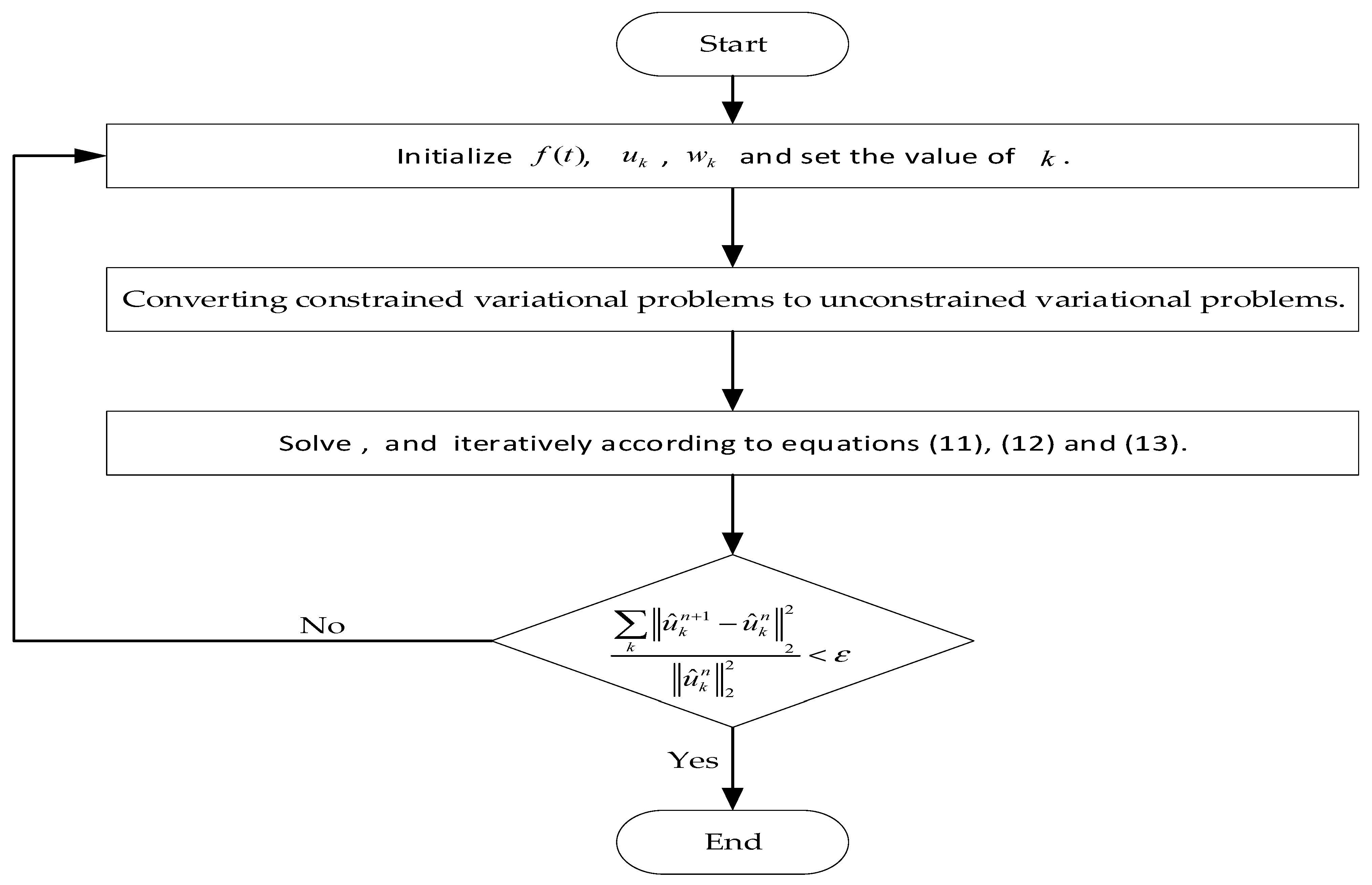
In many cases, due to the volatility of the signal data sequence, we need to decompose the signal sequence into a series of smooth subsequences in order to better perform subsequent processing. There are many commonly used decomposition methods, for example, EMD and EEMD decomposition methods, but all these methods have some limitations. In 2014, Dragomiretskiy et al. proposed a completely non-recursive variational modal decomposition method (VMD), which adaptively decomposes complex timing signals into several simple modal components [44]. The VMD algorithm is an effective method for applying the traditional Wiener filter to multiple adaptive bands, which has a broad theoretical basis and is easy to implement. VMD decomposition is a way to convert complex mathematical problems into simple mathematical expressions by building variational problems, finding the best solution, and improving the performance of the model using alternating direction multipliers to improve sampling accuracy. The calculation flow of VMD is shown in Figure 3. The specific steps are as follows.

(1)

Constructing variational problems.

Suppose the original input signal $f(t)$ is decomposed into $k$ components $u$. In order to ensure that the decomposed sequence is a modal component with a finite bandwidth of the central frequency, the sum of the estimated bandwidths of each modal component is required to be minimal, and the constraint is that the sum of all modal components should be equal to the original signal. The corresponding expression for the constrained variational problem is as follows:

$$\underset{\left\{u_k\right\}\left\{w_k\right\}}{{\displaystyle \min }}\left\{{\displaystyle \sum _k{\Vert {\partial }_t\left[\delta (t)+\frac{j}{\pi t}\right]\times u_k(t)e^{-j{w}_{k}t}\Vert }_2^2}\right\}$$

(8)

$$s_{·}{t}_{·}{\displaystyle \sum _k{u}_k}=f(t)$$

(9)

where $f(t)$ denotes the original signal, $k$ is the predetermined number of modal components, ${\partial }_t$ is the Dirac distribution function, $u_k=\left\{u_1,u_2,\cdots ,u_k\right\}$ is the $k$ modal components obtained from the adaptive decomposition of the original signal, and $w_k=\left\{w_1,w_2,\cdots ,w_k\right\}$ is the central frequency of each modal component.

(2)

Transformation of variational problems.

By using the quadratic penalty term $\alpha$ and the Lagrangian operator $\lambda (t)$, we can convert the variational problem with constraints into a problem with unconstrained variation by the following equation:

$$L(\{u_k\},\{{\omega }_k\},\lambda ):=\alpha {{\displaystyle \sum _k\Vert {\partial }_t\left[(\delta \left(t\right)+\frac{j}{\pi t})\times u_k(t)\right]e^{-j{w}_{k}z}\Vert }}_k^2+{\Vert f(t)-{\displaystyle \sum _k{u}_k(t)}\Vert }_2^2+\langle \lambda (t),f(t)-{\displaystyle \sum _k{u}_k(t)}\rangle$$

(10)

(3)

Solve the variational problem.

By using the alternating direction multiplier method (ADMM), we can solve the initial minimization problem. The Fourier isometric transform is used to obtain the results of the sequence decomposition in the frequency domain. $u_k^{n+1}$, ${\omega }_k^{n+1}$, and $\lambda$ are solved iteratively by searching the saddle points of the increasing Lagrangian function with the following equation:

$${\widehat{u}}_k^{n+1}(\omega )=\frac{\widehat{f}(\omega )-{\displaystyle \sum _{i\ne k}\widehat{u}(\omega )+\frac{\widehat{\lambda }(\omega )}{2}}}{1+2\alpha {(\omega -{\omega }_k)}^2}$$

(11)

$${\omega }_k^{n+1}=\frac{{\displaystyle {\int }_0^{\infty }\omega {\left|\widehat{u}(\omega )\right|}^{2}d\omega }}{{\displaystyle {\int }_0^{\infty }{\left|{\widehat{u}}_k(\omega )\right|}^{2}d\omega }}$$

(12)

$${\widehat{\lambda }}^{n+1}(\omega )={\widehat{\lambda }}^n(\omega )+\tau (\widehat{f}(\omega )-{\displaystyle \sum _k{\widehat{u}}_k^{n+1}(\omega )})$$

(13)

where ${\widehat{u}}_k^{n+1}(\omega )$ is the kth modal component with the center frequency of $\omega$ at the (n + 1) th iteration. ${\omega }_k^{n+1}$ is the center frequency of the kth modal component during the (n + 1) iteration. $\tau$ is the noise tolerance of the signal.

After repeated iterations until the convergence condition is reached or the maximum number of iterations is reached and stopped, the convergence condition can be expressed as:

$$\frac{{{\displaystyle \sum _k\Vert {\widehat{u}}_k^{n+1}-{\widehat{u}}_k^n\Vert }}_2^2}{{\Vert {\widehat{u}}_k^n\Vert }_2^2}<\epsilon$$

(14)

2.3. Fuzzy Entropy (FE)

Fuzzy entropy was proposed by Chen et al. in 2007 and was originally intended for use in myoelectric model processing, although it has since been widely used in areas such as fault diagnosis and image processing [45]. FE is a valid measure of time series complexity, and it can reflect the complexity of the data more accurately by improving the sample entropy and approximate entropy. The FE algorithm calculates the entropy value of the time series by introducing a de-meaning operation that defines the similarity of the vectors in the phase space reconstruction formula as an exponential function. The increase in the FE value implies an increase in the complexity of the time series. The steps of its algorithm are as follows:

(1)

Knowing an $N$-dimensional time series $[\mu (1),\mu (2),\cdots ,u(N)]$, let the phase space dimension be $m(m\le n-2)$ and the phase space vector be:

$$X_i=[\mu (i),\mu (i+1),\cdots ,\mu (i+m-1)]-{\mu }_0(i),i=1,2,\cdots ,N-m+1$$

(15)

where ${\mu }_0(i)=\frac{1}{m}{\displaystyle \sum _{j=0}^{m-1}\mu (i+j)}$ denotes the spatial mean.

(2)

The maximum difference between the corresponding elements of $X_i$ and $X_j$ is defined as the distance $d_{i,j}^m$.

$$d_{i,j}^m=d[X_i,X_j]=\max \left[\left|\mu (i+p)-{\mu }_0(i)-(\mu (j+p)-{\mu }_0(j))\right|\right],p=1,2,\cdots ,m-1$$

(16)

(3)

Introduce the affiliation function as the following equation:

$$A(x)=\{\begin{array}{cc}1& x=0\\ \exp [-\ln (2){(\frac{x}{r})}^n]& x>0\end{array}$$

(17)

where $r$ is the similar tolerance boundary width and $n$ is the similar tolerance boundary gradient.

For the phase space, there is Equation (18).

$$A_{i,j}^m=\exp \left[-\ln (2){\left(\frac{d_{i,j}^m}{r}\right)}^n\right],j=1,2,\cdots ,N-m+1,j\ne i$$

(18)

(4)

Define the function.

$$C_i^m(n,r)=\frac{1}{N-m}{\displaystyle \sum _{j=1,j\ne i}^{N-m+1}{A}_{i,j}^m}$$

(19)

(5)

Define the function.

$${\varphi }_i^m(r)={(N-m+1)}^{-1}{\displaystyle \sum _{i=1,j\ne i}^{N-m+1}{C}_i^m(n,r)}$$

(20)

(6)

When $N$ is a finite value, the value of FE can be expressed as Equation (21).

$$FE(m,n,r)=\ln {\varphi }_i^m(n,r)-\ln {\varphi }_i^{m+1}(n,r)$$

(21)

From the above, it can be seen that the size of the entropy value is related to the length of the data $N$ and the parameters $m$, $r$, $n$, and $r$ are generally taken as $0.1\sim 0.5{\sigma }_{SD}$ (${\sigma }_{SD}$ is the standard deviation of the original sequence), and $n$ plays a weighting role in the vector calculation of similarity and is generally taken as a smaller number (e.g., 1 or 2).

2.4. The Temporal Convolutional Network (TCN)

The TCN, as a new architecture based on convolutional neural networks (CNNs), can not only solve the problem of excessive time consumption by parallel computation but is also different from the CNN because the TCN is composed of causal convolution, dilated casual convolution, and residual block structure.

2.4.1. Causal Convolution

Causal convolution is used in the TCN network. Suppose that a given input sequence $x_1,x_2,\cdots ,x_t$ is used to predict $y_1,y_2,\cdots ,y_t$. The output of the predicted value $y_t$ at the current moment in the causal convolution is only related to the input $x_t$ at the current moment and the input at the previous moment, which is also consistent with the impossibility of knowing future information in advance on the prediction problem. It can be expressed as the following:

$$y_t=f\left(x_1,x_2,\cdots ,x_t\right)$$

(22)

where $f(·)$ denotes a convolution operation.

2.4.2. Dilated Casual Convolution

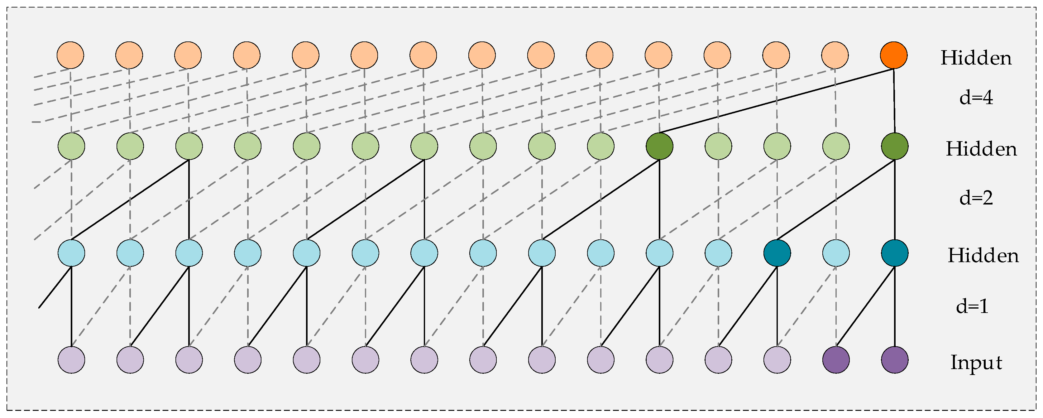
The historical data captured by causal convolution are only linearly related to the depth of the network, so the older the historical information traced, the more hidden layers it leads to. Thus, using a simple causal convolution does not capture a long time series. Therefore, the dilated causal convolution technique is used in the TCN to improve efficiency. The dilated causal convolution injects holes into the standard causal convolution, which allows the dilated causal convolution to obtain a larger perceptual field without changing the size of the convolution kernel and reduces the depth of the causal convolution without increasing the number of parameters. The structure of the dilated convolution is shown in Figure 4.

Assume that the one-dimensional sequence input to the temporal convolutional network is $x\in R^n$ and the convolutional kernel is $f:\{0,\dots ,k-1\}\to R$. Define the null causal convolution operation $s$ on the elements $F$ in the sequence as follows:

$$F(s)=(x\ast {}_{d}f)(s)={\displaystyle \sum _{i=0}^{k-1}f(i)}\cdot x_{s-d_i}$$

(23)

where $d_i$ is the dilation factor of the $i$-th layer convolution, $k$ is the size of the convolution kernel, and $s-d_i$ is the direction of the sequence past time. Usually, as the number of layers increases, the dilation factor $d$ grows exponentially by 2. The larger $d$ is, the larger the input range is, thus increasing the perceptual field of the convolutional network, and when $d=1$, it is the standard causal convolution.

2.4.3. Residual Block

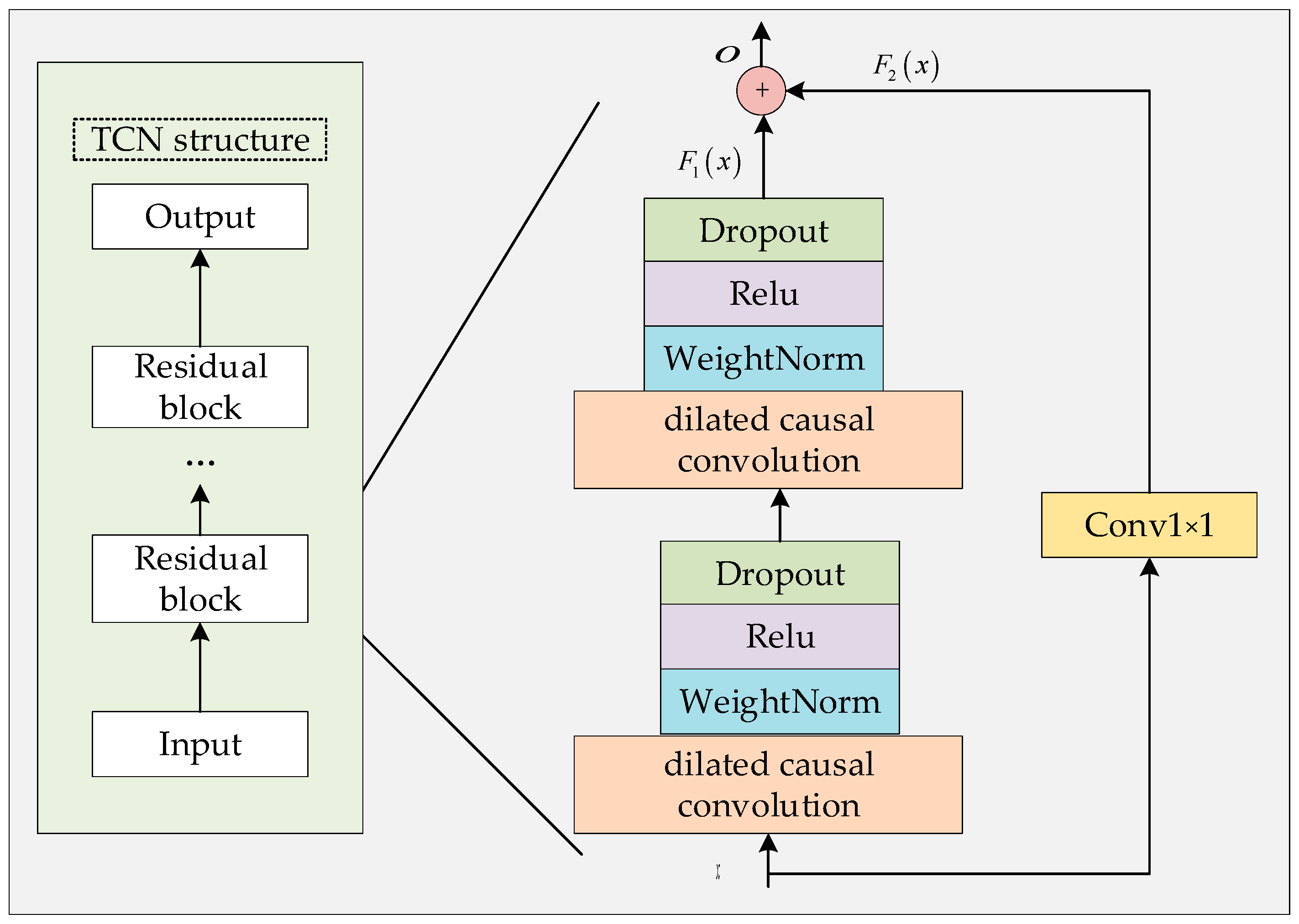
To increase the perceptual field, the TCN is implemented by increasing the convolutional kernel, increasing the expansion factor, and stacking the number of network layers, which deepens the network depth. However, a deeper network structure may cause problems, such as gradient disappearance, for which the residual block is introduced in the TCN. The relationship between the input $x$ and output $o$ of the residual block is shown in Equation (24), and the structure of the residual block is shown in Figure 5.

$$o=Activation\left(F_1\left(x\right)+F_2\left(x\right)\right)$$

(24)

where $x$ is the input of the residual block, $o$ is the output of the residual block, $Activation(\cdot )$ is the activation function, $F_1\left(x\right)$ is the output of the multilayer network, and $F_2\left(x\right)$ is the output of Conv1×1.

Each residual block contains a dilated causal convolution, Relu, WeightNorm, and Dropout, which together form the whole. The use of WeightNorm and Dropout techniques effectively prevents gradient disappearance and model overfitting. The advent of Conv1×1 greatly improves the performance of the network by allowing the network layers to learn constant mappings, thus effectively avoiding network degradation.

2.5. Temporal Pattern Attention (TPA)

The attention mechanism is inspired by an information processing mechanism derived from human vision. The core of the attention mechanism is to assign different weights to the input feature information, focus on important information, and ignore irrelevant information, so as to capture the global and local connections, optimize the prediction model, and improve the prediction accuracy. The temporal pattern attention mechanism proposed by Shun-Yao Shih et al. [46] can effectively solve the problem that the traditional attention mechanism only relies on weighting the time steps, and it can also better consider multivariate time series and thus can more accurately predict the relationship between variables. The TPA model is shown in Figure 6.

In the model in this paper, TPA firstly extracts fixed-length temporal patterns from the output information of the implicit layer of the TCN through CNN filters, determines the weights of each temporal pattern using a scoring function, and fuses the final output information according to the magnitude of the weights, as follows.

(1)

The TCN processing time series.

The original multivariate time series is processed using TCN to obtain the hidden state $h_i$ (column vector) for each time step, where each $h_i$ has dimension $m$ and $w$ is the length of the time window representing the selected range of historical data to obtain the hidden state matrix $H=\left\{h_{t-w},h_{t-w+1},\cdots ,h_{t-1}\right\}$ and the hidden state $h_t$ at the last moment.

(2)

CNN convolution.

$k$ convolution kernels ($1\times w$) are used to capture the signal patterns with variable hidden states, with the following equation:

$$H_{i,j}^C={\displaystyle \sum _{l=1}^w{H}_{i,(t-w-1+l)}\times C_{j,T-w+l}}$$

(25)

(3)

The attention weight.

Let $query=h_t$, $key=H^C$, then $Scoring\mathrm{Function}$ is:

$$f(H_i^C,h_t)={(H_i^C)}^T{W}_a{h}_t$$

(26)

The attention weight ${\alpha }_i$ is obtained by normalizing using the sigmod function, as in the following equation:

$${\alpha }_i=sigmoid(f(H_i^C,h_t))$$

(27)

Using the attention weight ${\alpha }_i$, a weighted summation is performed for each row $H^C$ to obtain the context vector $v_t$, as in the following equation:

$$v_t={\displaystyle \sum _{i=1}^m{\alpha }_i{H}_i^C}$$

(28)

(4)

Fusion.

Finally, $v_t$ and $h_t$ are fused and the output of the attention layer is obtained by linear transformation:

$$h_t^{\prime }=W_h{h}_t+W_v{v}_t$$

(29)

$$y_{t-1+\Delta }=W_{h^{\prime }}{h}_t^{\prime }$$

(30)

3. The Proposed EPT-VMD-TPA-TCN Model and the Restructured EPT-VMD-FE-TPA-TCN Model

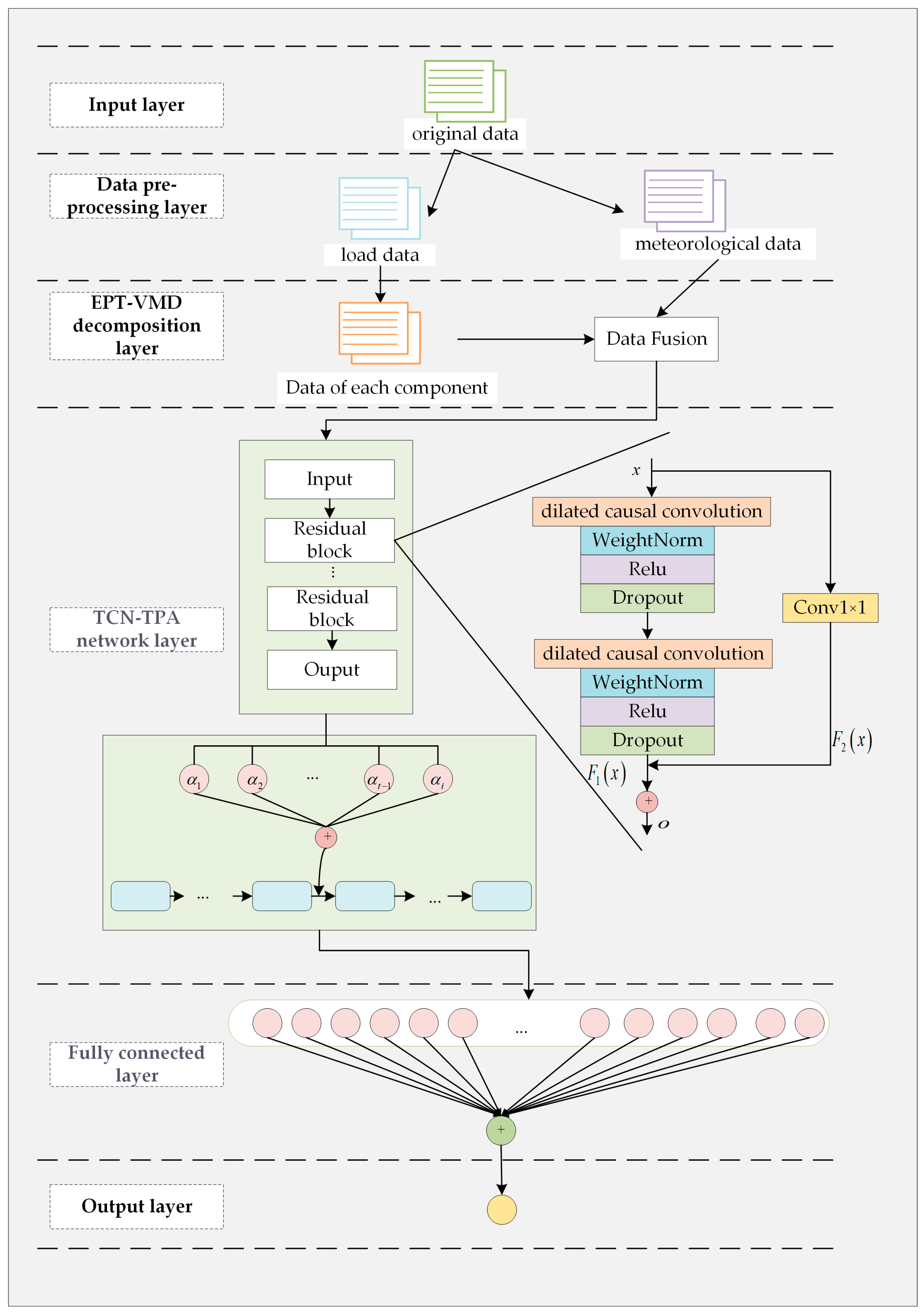
In this paper, we propose a short-term power load forecasting model (EPT-VMD-TCN-TPA) based on the mixed decomposition of load data and TCN-TPA network forecasting. The Tr(t) component and Re(t) component of the load series are first extracted using EPT. Then, the Re(t) component is decomposed into several IMFs with different center frequencies using VMD, and the Tr(t) component and each IMF component are fused with weather and other influencing factors separately. Finally, the TCN-TPA network model is used to train and predict the data. The reorganization model EPT-VMD-FE-TPA-TCN discussed in this paper is based on the EPT-VMD-TPA-TCN model and uses the concept of fuzzy entropy (FE) to calculate the complexity of each IMF component. The IMF components of similar complexity are combined into a new component (FE-IMF), and finally, the TCN-TPA network is used to train and predict each fused weather factor FE-IMF component and Tr(t) component. The structural framework of the EPT-VMD-TPA-TCN prediction model proposed in this paper is shown in Figure 7.

The EPT-VMD-TCN-TPA prediction model proposed in this paper can be divided into three key parts: the EPT-VMD decomposition layer, the TCN-TPA network training and prediction layer, and the fully connected prediction result output layer. The EPT-VMD-FE-TCN-TPA recombination prediction model is added with the FE subsequence recombination layer after the EPT-VMD decomposition layer. This section details the key components of the experimental dataset and model.

3.1. Experimental Datasets

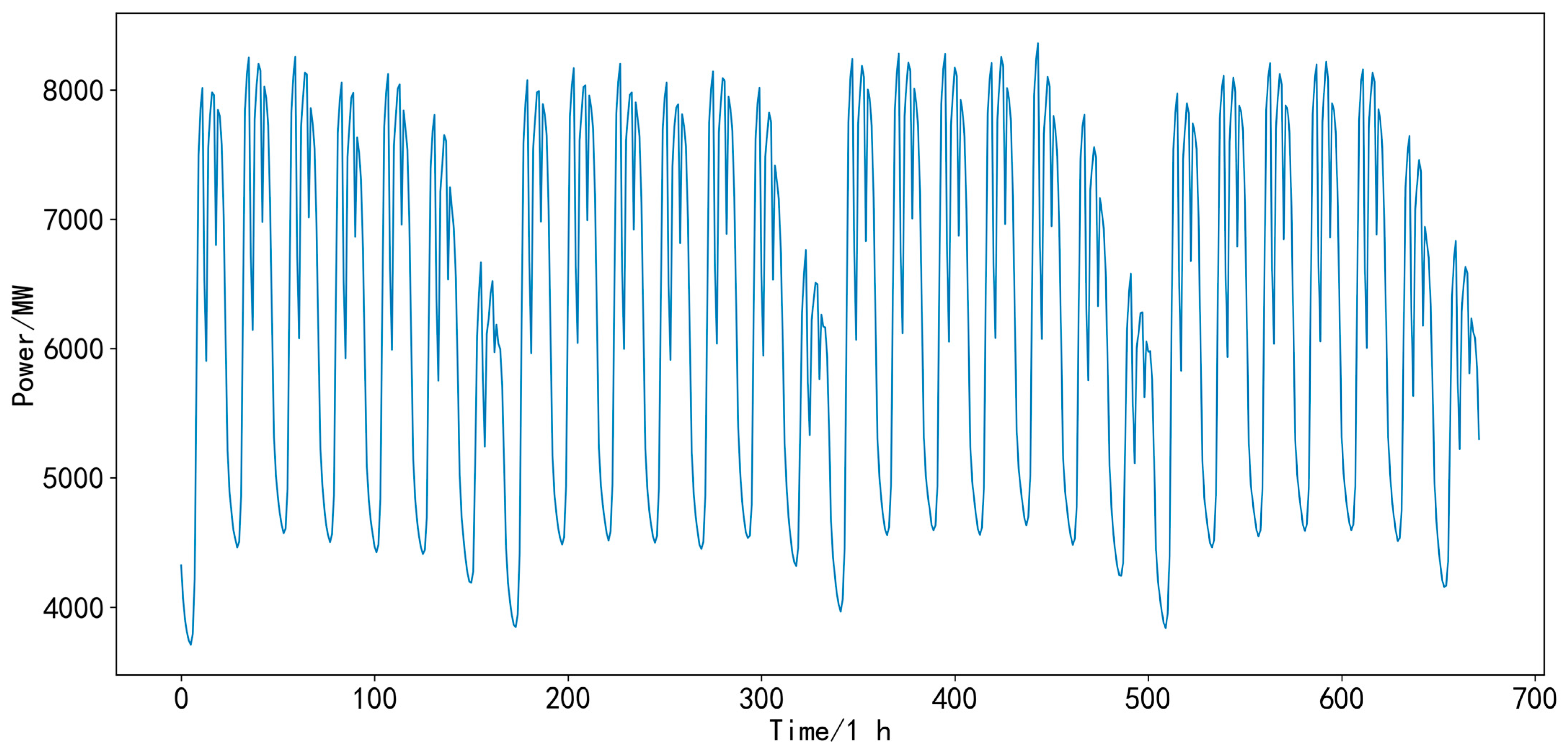
In this paper, the datasets of Area 1 and Area 2 provided by the 9th National Electrician Mathematical Modeling Competition in China are used as the experimental data sources. The data for each Area include load data and meteorological data between 1 January 2012 and 10 January 2015. The electrical load sampling interval was 15 min, and 96 points were taken per day in MW. The meteorological data include daily maximum temperature, minimum temperature, average temperature, rainfall, and relative humidity. The data from Area 1 are used as the main dataset for the experiment, and the dataset from Area 2 is used to verify the scalability of the prediction model proposed in this paper. In each Area, the first 80% of the data were used as the training set and the last 20% were used as the test set. The original load data series of Area 1 are shown in Figure 8. The trend of Area 1’s continuous four-week load data is shown in Figure 9. The load data statistics are shown in

Table 1. Dataset load details.

Dataset	Samples	Range	Numbers	Mean (MW)	Max (MW)	Min (MW)	Std. (MW)
Area 1	All samples	1 January 2012–10 January 2015	106,176	6915.33	12,296.85	1306.08	2094.08
	Training	1 January 2012–2 June 2014	84,864	6657.81	11,446.85	1306.08	2034.47
	Testing	3 June 2014–10 January 2015	21,312	7945.53	12,296.85	2267.67	2010.75
Area 2	All samples	1 January 2012–10 January 2015	106,176	7357.43	13,536.74	1986.32	2180.43
	Training	1 January 2012–2 June 2014	84,864	7038.44	12,466.10	1986.32	2054.60
	Testing	3 June 2014–10 January 2015	21,312	8627.67	13,536.74	3259.12	2204.07

. The meteorological data for one week in Area 1 are described in

Table 2. Data of meteorological factors from 1 August to 7 August 2012 (Area 1).

Date	Max. Temperature (°C)	Min. Temperature (°C)	Avg. Temperature (°C)	Relative Humidity (avg.)	Rainfall (mm)
1 August 2012	36.0	23.1	30.3	71.0	26.5
2 August 2012	35.6	27.8	31.9	61.0	0.0
3 August 2012	33.9	28.0	30.9	63.0	0.0
4 August 2012	31.3	27.8	29.5	75.0	0.0
5 August 2012	31.0	26.2	28.5	82.0	1.8
6 August 2012	30.8	24.7	26.9	87.0	12.3
7 August 2012	34.5	25.8	29.4	79.0	0.1

(only 1 August 2012–7 August 2012 are shown).

(1)

Dataset (Area 1): 1 January 2012–10 January 2015 (total 1106 days, 106,176 load data collection points).

(2)

Training set: data from 1 January 2012–2 June 2014 (884 days, 84,864 load data collection points) were used to train the model.

(3)

Test set: 3 June 2014–10 January 2015 (222 days, 21,312 load data sampling points) was used for the evaluation of the model.

Throughout the training and prediction process of the model, a sliding window training method is used, i.e., load data from the past consecutive week (168 h) and weather data are always selected to predict the future day’s load, and for each completed training, the data used for training are pushed back 24 h for the next model training.

According to Figure 8 and Figure 9, it can be seen that the power load data have obvious periodic characteristics and also show strong fluctuation. Let the original load data in the dataset be $f\left(t\right)$ and the meteorological data be $m\left(t\right)$. The load forecast is determined by both the historical load data $f\left(t\right)$ and meteorological data $m\left(t\right)$. Since the load data have strong volatility and periodicity, this paper will first process the load data, and then the processed data will be fused with the meteorological data. Finally, the fused data will be trained and predicted using the TCN-TPA network model. The processing of the load data will be described in detail below.

3.2. EPT-VMD Decomposition Layer

3.2.1. EPT Decomposition

From the previous analysis of the dataset, it is clear that the load data are not only non-stationary but also have a certain periodicity. If the VMD is used directly to decompose it, the trend of the load series will not be extracted. In this paper, we use EPT to process the load data f and extract the trend of the original load series, so as to obtain the trend component t and the fluctuation component R. The results of decomposing the load data series of Area 1 by using EPT are shown in Figure 10. The results of decomposing the load data series of Area 2 by using EPT are shown in Figure 11.

In Figure 10 and Figure 11, it can be seen that the Tr(t) component obtained using EPT extraction has a strong periodicity and regularity for both Area 1 and Area 2. The Re(t) component has non-smoothness and needs further processing to obtain a relatively smooth subsequence.

3.2.2. VMD

In the experiment, in order to reduce the volatility and randomness of the Re(t) component, VMD is used to decompose it so as to obtain several relatively smooth IMF components. According to Section 2.2, the number of IMFs, i.e., the value of $k$, must be determined before using VMD to decompose Re(t). If the value of $k$ is too small, the decomposition result is inadequate and increases the error of prediction. If the value of $k$ is too large, the decomposition is overdone, thus increasing the overhead of the decomposition. In this paper, we will use the method in reference [47] to determine the number $k$ of the decomposed modal functions using the decomposed residuals (R_res), as in Equation (31):

$$R_{res}=\frac{1}{M}{\displaystyle \sum _{t=1}^M\left|\frac{Tr\left(t\right)-{\displaystyle {\sum }_{i=1}^k{u}_i(t)}}{Tr\left(t\right)}\right|}$$

(31)

where Re(t) is the residual fluctuation component, $u_i(t)$ is the IMF subsequence obtained by VMD decomposition, the number of samples is $M$, and the number of IMF subsequences is $k$.

In this paper, when the value of R_res is less than 1% and there is no obvious downward trend, the value of $k$ is the appropriate number of decompositions for VMD. The results of the $\mathrm{Re}(t)$ decomposition using different values of $k$ are shown in

Table 3. R_res-values corresponding to different $k$ values.

k	Rres-Value of Area 1	Rres-Value of Area 2
2	0.01588381	0.01149027
3	0.01077131	0.01032953
4	0.00584849	0.00780275
5	0.00502476	0.00628756
6	0.00412682	0.00523697
7	0.00386909	0.00402301
8	0.00370431	0.00331197
9	0.00360939	0.00285365
10	0.00356238	0.00239487
11	0.00338015	0.00198062
12	0.00335977	0.00197231
13	0.00334251	0.00197134
14	0.00333611	0.00197128
15	0.00332795	0.00197123

.

As can be seen in Table 3, in Area 1, when the value of $k$ is 11, R_res = 0.00338015 < 0.001, and when $k>11$, the decreasing trend of R_res tends to be stable. In Area 2, when the value of $k$ is 11, R_res = 0.00198062 < 0.001, and when $k>11$, the decreasing trend of R_res tends to be stable. In this paper, the VMD algorithm has a penalty function $\alpha =1000$, a noise tolerance $\tau =0$, and a convergence tolerance $\epsilon =1\times {10}^{-6}$.

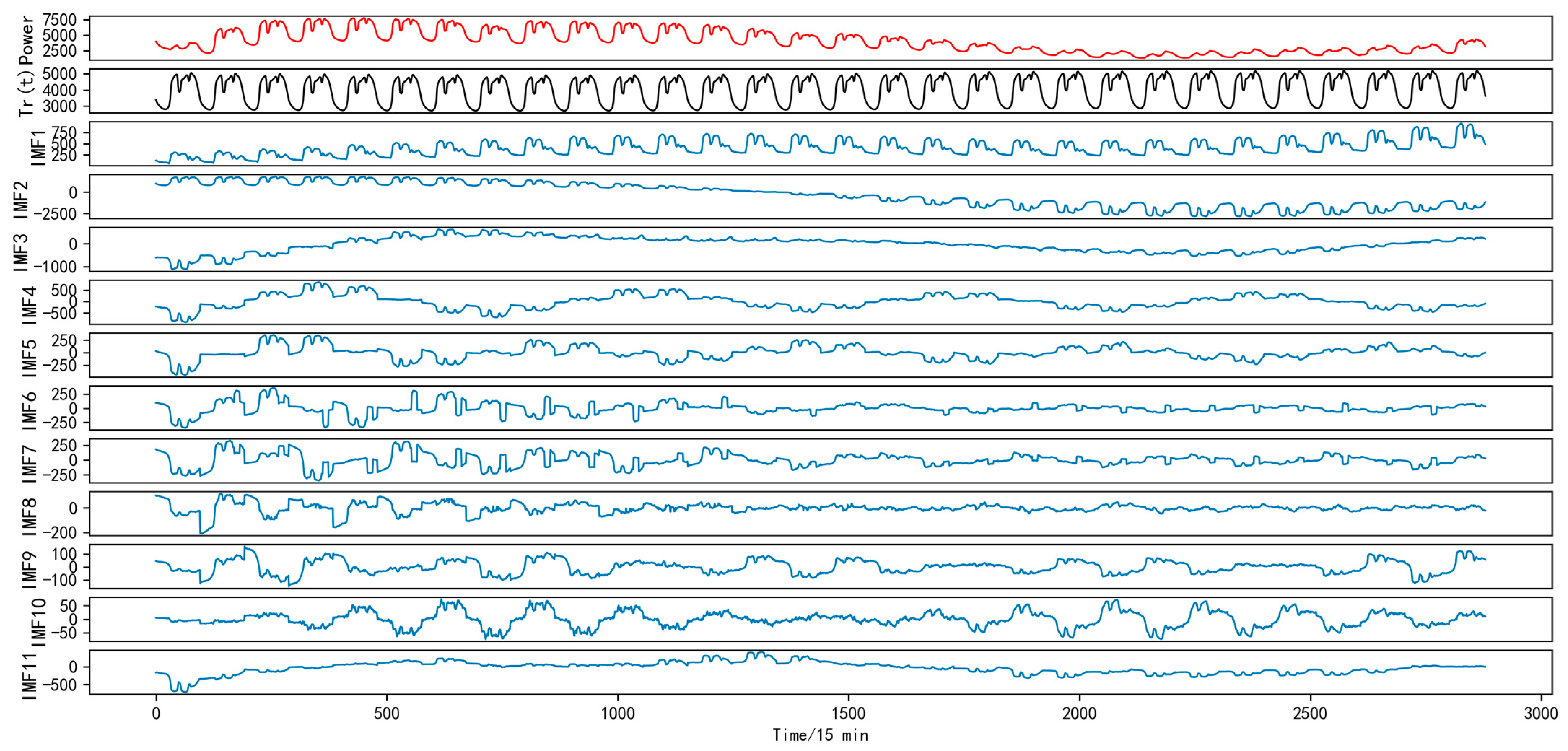
When $k$ is taken as 11, Figure 12 shows the results of the decomposition of the residual volatility component using VMD for the first month in Area 1. Figure 13 shows the results of the decomposition of the residual volatility component using VMD for the first month in Area 2.

As can be seen in Figure 12, the use of EPT and VMD for the electric load series not only extracts the trend component of the original load series but also VMD decomposes the fluctuating component series into smoother sub-series. In Area 2, Figure 13 similarly shows that the hybrid EPT-VMD decomposition method proposed in this paper is more effective.

3.3. Sub-Sequence Recombination Layer

The content in this subsection is part of a restructured model (EPT-VMD-FE-TPA-TCN) based on the proposed EPT-VMD-TPA-TCN prediction model in this paper. Since the central frequencies of each IMF component obtained by decomposing the fluctuating components using VMD are different, these IMFs will have different effects on load forecasting. Moreover, too many components from VMD decomposition will increase the time consumption of the prediction model. In this paper, we will apply fuzzy entropy to calculate the complexity of each IMF component in the EPT-VMD-FE-TPA-TCN reorganization prediction model and combine and reorganize the IMF components with similar fuzzy entropy values into a new component (FE-IMF).

In this paper, the fuzzy entropy values are calculated by taking the sequence length $\mathrm{N}$ as the total sample length, the phase space dimension $m=2$, the similarity tolerance limit $r=0.3S_d$, and $n=2$. The fuzzy entropy values of each IMF component are shown in Figure 14.

In Figure 14, we can see that the fuzzy entropy of IMF components varies widely but there are some components with similar fuzzy entropy values, which indicates that there is some similarity among them. The fuzzy entropy of IMF1 is significantly lower than other components, while the fuzzy entropy of IMF7 is the highest. The IMF components with similar fuzzy entropy values are reorganized, as shown in

Table 4. FE-IMF composition.

Recombinant Sequences	FE-IMF1	FE-IMF2	FE-IMF3	FE-IMF4	FE-IMF5	FE-IMF6
Components	IMF1	IMF2	IMF3 + IMF10	IMF4 + IMF7	IMF5 + IMF6	IMF8 + IMF9 + IMF11

.

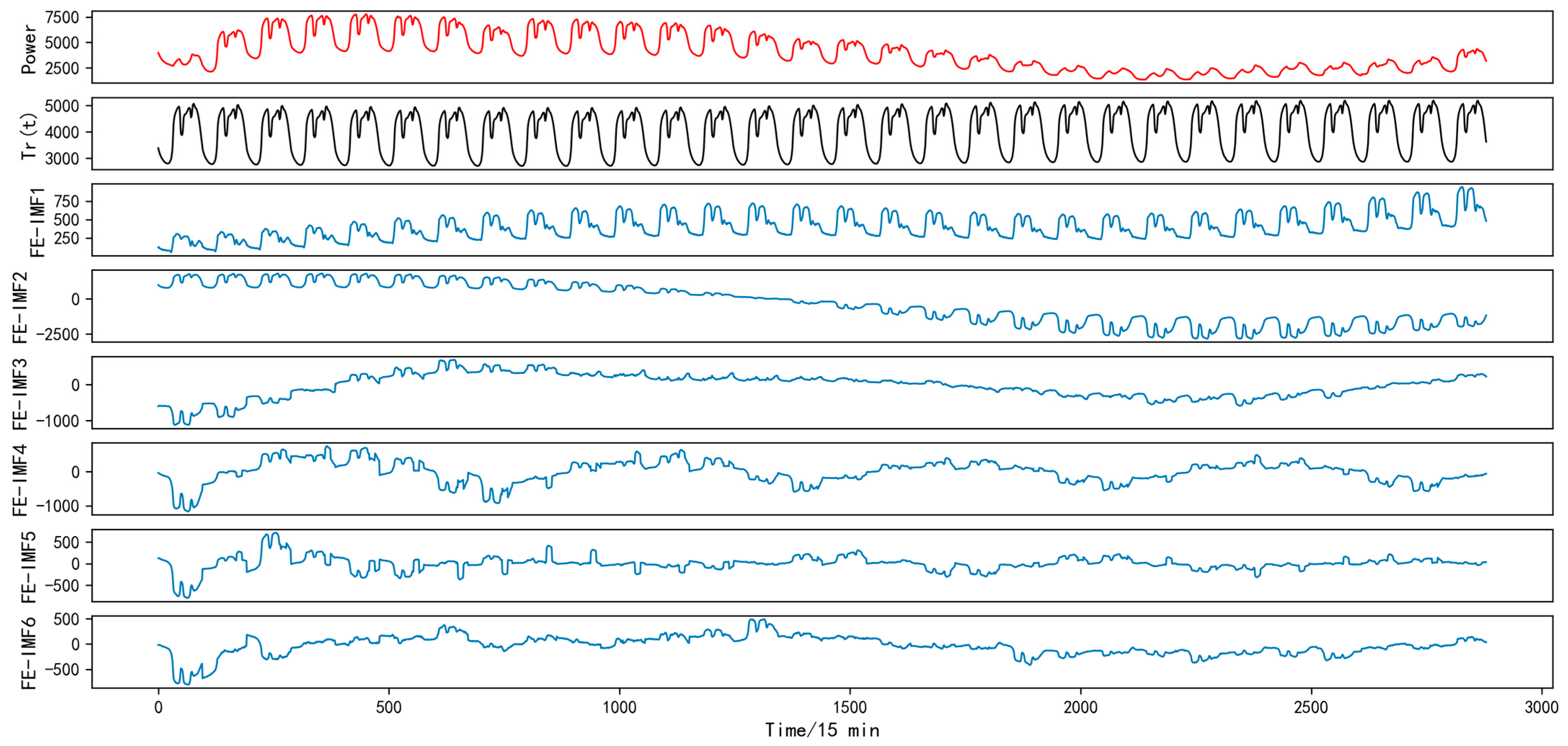
A comparison of the original load series of the first month in Area 1 and the series after decomposition by EPT-VMD and reorganization by FE is shown in Figure 15. From the comparison in Figure 15, it can be seen that the trend component of the original load series can be advanced by EPT, the remaining fluctuation component can be decomposed into relatively stable IFM components by VMD, and the number of components is reduced by using FE to combine IMF components with similar fuzzy entropy values into FE-IMF.

3.4. TCN-TPA Network Training and Prediction Layers

Short-term power load forecasting is a multivariate time series task because short-term power load forecasting is not only related to historical load but also to variables such as meteorological factors. For this multivariate time series forecasting task, this paper will use the TCN-TPA network model for short-term power load forecasting. Firstly, the TCN network can not only control the memory length of the model by adjusting the expansion rate and changing the convolutional kernel but also the TCN network has the ability to process data in a massively parallel way, which makes the training and validation time of the prediction model shorter. Secondly, using the temporal attention mechanism not only allows assigning different weights to the input information to highlight the key influencing factors but also breaks away from the typical attention mechanism’s tendency to select time steps that are more relevant to time series prediction. The temporal attention mechanism can better capture temporal information and span multiple time steps so that temporal patterns can be extracted for each load component and focus on relevant meteorological factors to improve prediction precision.

3.5. Fully Connected Prediction Result Output Layer

The fully connected layer can obtain output information from the TCN-TPA layer to obtain prediction results for multiple components. By inverse normalizing the prediction results of each component of the fully connected layer and superimposing them, accurate load prediction results can be obtained.

3.6. Workflow of the EPT-VMD-TCN-TPA Model

In this paper, an EPT-VMD-TCN-TPA short-term electric load forecasting model is proposed. The EPT-VMD-FE-TCN-TPA forecasting model is discussed on the basis of the EPT-VMD-TCN-TPA model. The workflow of the proposed EPT-VMD-TCN-TPA model is shown in Figure 16, and each step is described as follows:

Step 1: Pre-processing of the raw data.

Step 2: The pre-processed raw data are divided into load data $f(t)$ and meteorological data $m(t)$.

Step 3: Use EPT to extract the trend component (Tr(t)) and the residual fluctuation component (Re(t)) of the load data $f(t)$.

Step 4: The residual fluctuation components are decomposed into IMF components using VMD according to the predefined $k$ values.

Step 5: Each IMF component and Tr(t) component is fused with $m(t)$ separately and the fused data are normalized to eliminate the effect of different dimensional data.

Step 6: The data fused in Step 5 are divided into a training set and a test set. The training set is fed into the TCN-TPA network and the hyperparameters of the model are improved and updated by calculating the loss function MSE to learn the complex relationships between the input and output variables in each subsequence.

Step 7: Each subsequence is predicted using the trained TCN-TPA network, and the prediction result of each subsequence is derived by the fully connected layer.

Step 8: The prediction results of each sub-series are summed up by the inverse normalization process, and the final accurate prediction result of the load is obtained.

The EPT-VMD-FE-TCN-TPA prediction model is added with the recombination operation after step 4. That is, the fuzzy entropy (FE) values of each IMF component are calculated and the IMFs with similar values are reorganized to obtain each reorganization component (FE-IMF).

4. Experiments

4.1. Datasets and Experimental Environment

The dataset was analyzed and described in Section 3.1. The experiments in this paper were performed with Python 3.8 running on 64-bit Windows 10 and the open-source library vmdpy to write the VMD programs. The models were developed using the Keras-based TesorFlow framework. The neural network was implemented in Keras 2.11. The environment parameters are shown in

Table 5. Experimental environment parameters.

Processor	Memory	Python	TensorFlow	Keras
Intel(R) Core (TM) i5-7200U CPU @ 2.50 GHz 2.70 GHz	4 G	3.8	2.11.0	2.11.0

.

In the TCN-TPA prediction model in this paper, the hyperparameters are the number of convolution kernels, convolution kernel size, dilation rate, number of iterations, number of TCN residual blocks, dropout, and batch size. The number of convolutional kernels is set to (10,20,32,64), the size of the convolutional kernels is set to (1,2,3,4,5), the expansion factor is set to (1,2,4,8), the number of TCN residual blocks is set to (1,2,3), and the batch size is set to (16,32,64,128). In this paper, we used the GridSearchCV method from the Sklearn library in Python to perform the grid search for these hyperparameters [48] using MSE as the loss function, a learning rate set to 0.001, and an Adam optimizer to optimize the parameters. The hyperparameters shown in

Table 6. Model parameters (1).

Items	Number of Residual Blocks	Convolution Kernel Size	Number of Convolution Kernels	Dilation Rate	Number of Iterations	Dropout
Value	3	3	20	(1,2,4)	100	0.1

and

Table 7. Model parameters (2).

Items	Learning Rate	Loss Function	Optimizer	Activation Functions	Batch-Size
Value	0.001	MSE	Adam	ReLU	64

are obtained experimentally.

4.2. Data Normalization

In the EPT-VMD-TCN-TPA prediction model proposed in this paper, the original data are divided into load data $f(t)$ and meteorological data $m(t)$, where the trend component Tr(t) and the residual fluctuation component Re(t) are obtained by EPT operation on the load data $f(t)$. The Re(t) component is decomposed into $k$ IMF components by VMD, and the result is denoted as $d_i(t)$, $i=1,2,3\cdots k.$ (where $k$ is the number of IMF components).

The Tr(t) and the $m(t)$ are fused and denoted as $Ft=F(Tr,m)$.

The fusion of components $d_i(t)$ and $m(t)$ are denoted as $F_{i}t=F(d_i,m)$ (where $i=1,2,3\cdots k$, $k$ is the number of IMF components).

The fused $Ft$ and $F_{i}t$ are normalized and the normalized components are input into the prediction model, and through experiments, we can then accurately predict the value of the load. The final load prediction result consists of the superposition of the Tr(t) component and each IMF component prediction result, as shown in Equation (32):

$$P_{real}=P_{Ft}+{\displaystyle \sum _{i=1}^n{P}_{F_{i}t}}$$

(32)

where $p_{real}$ is the final forecasted value of the electric load, $P_{Ft}$ is the resultant value of the trend component forecast, and $P_{F_{i}t}$ is the resultant value of the IMF component forecast.

In order to eliminate the adverse effects of numerical bias on the model performance and speed up the training of the model, this paper will use the maximum–minimum normalization method to normalize the fused data $Ft$ and $F_{i}t$. The normalization formula is shown in Equation (33):

$$x^{*}=\frac{x-x_{\min }}{x_{\max }-x_{\min }}$$

(33)

where $x$ represents the fused sample data, $x^{*}$ is the normalized data, $x_{\min }$ is the minimum value in the sample data, and $x_{\max }$ is the maximum value in the sample data.

4.3. Error Evaluation Indicators

In this paper, we evaluate the error of the prediction results by using the mean absolute percentage error (MAPE), root-mean-square error (RMSE), mean absolute error (MAE), and R-squared (R²). The smaller the values of MAPE, RMSE, and MAE, the more accurate the load prediction results are, and the larger the value of R², the better the fit between the load prediction series curve and the actual load series curve is and the more accurate the prediction results are. This paper also performs a statistical test for all models, namely the Diebold and Mariano (DM) test [49]. The formula for the four evaluation indicators is defined as follows:

$$MAPE=\frac{1}{N}\frac{{\displaystyle {\sum }_{i=1}^N\left|{\widehat{y}}_i-y_i\right|}}{y_i}\times 100\%$$

(34)

$$RMSE=\sqrt{\frac{1}{N}{\displaystyle \sum _{i=1}^N{({\widehat{y}}_i-y_i)}^2}}$$

(35)

$$MAE=\frac{1}{N}{\displaystyle \sum _{i=1}^N\left|{\widehat{y}}_i-y_i\right|}$$

(36)

$$R^2=1-\frac{{\displaystyle \sum _{i=1}^N(y_i-{\widehat{y}}_i}{)}^2}{{(y_i-{\overline{y}}_i)}^2}$$

(37)

$${\overline{y}}_i=\frac{1}{N}{\displaystyle \sum _{i=1}^N{y}_i}$$

(38)

where $y_i$ is the actual value of the load, ${\widehat{y}}_i$ is the predicted value of the load, and $N$ the number of load sample points.

4.4. Ablation Experiments

In order to verify the prediction effect produced by each step of the combined model proposed in this paper, we will build the TCN model, the VMD-TCN model, the VMD-TCN-Attention model, the VMD-TCN-TPA model, the final proposed EPT-VMD-TCN-TPA model, and the EPT-VMD-FE-TCN-TPA recombination model in this paper, respectively. Among them, these models are briefly described as follows:

(1)

TCN model [27]: This model is a more advanced model in recent years, which not only can effectively extract the features of nonlinear time series data but also can effectively solve complex problems such as gradient explosion and gradient disappearance during model training.

(2)

VMD-TCN model: The load data are firstly decomposed using VMD, after which the dataset is trained and predicted using the TCN network.

(3)

VMD-TCN-Attention model: A general attention mechanism is added to the VMD-TCN model.

(4)

VMD-TCN-TPA model: Based on the VMD-TCN model, the prediction capability is improved by introducing a temporal pattern attention mechanism, which is especially suitable for handling multi-task temporal prediction.

(5)

EPT-VMD-TCN-TPA model: Our proposed final model. Before using the VMD-TCN-TPA model, the EPT method, which extracts the trend components of the load data, is first introduced.

(6)

EPT-VMD-FE-TCN-TPA model: This model adds a recombination layer to the proposed EPT-VMD-TCN-TPA model in this paper and merges the similar components of the intermediate processes according to FE values.

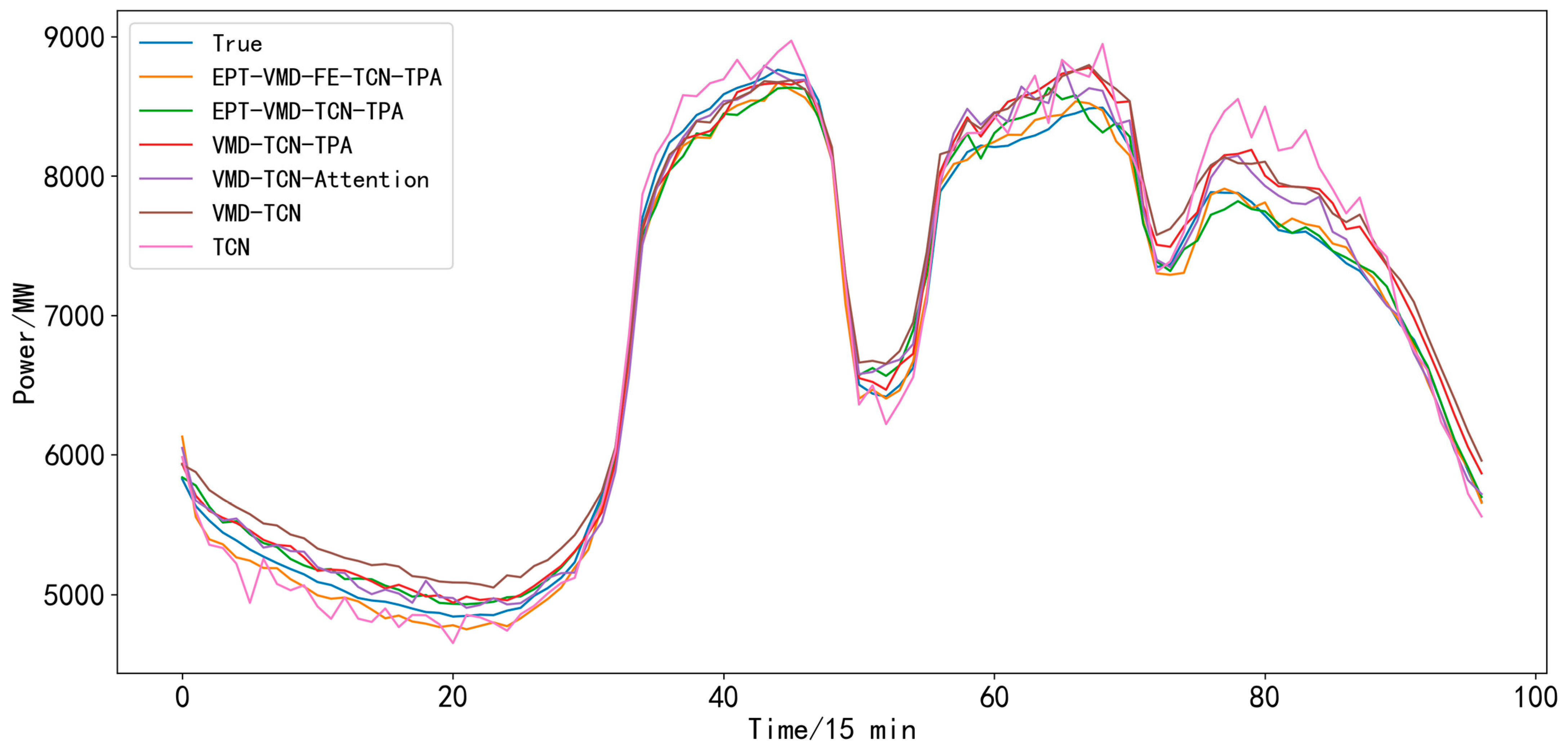
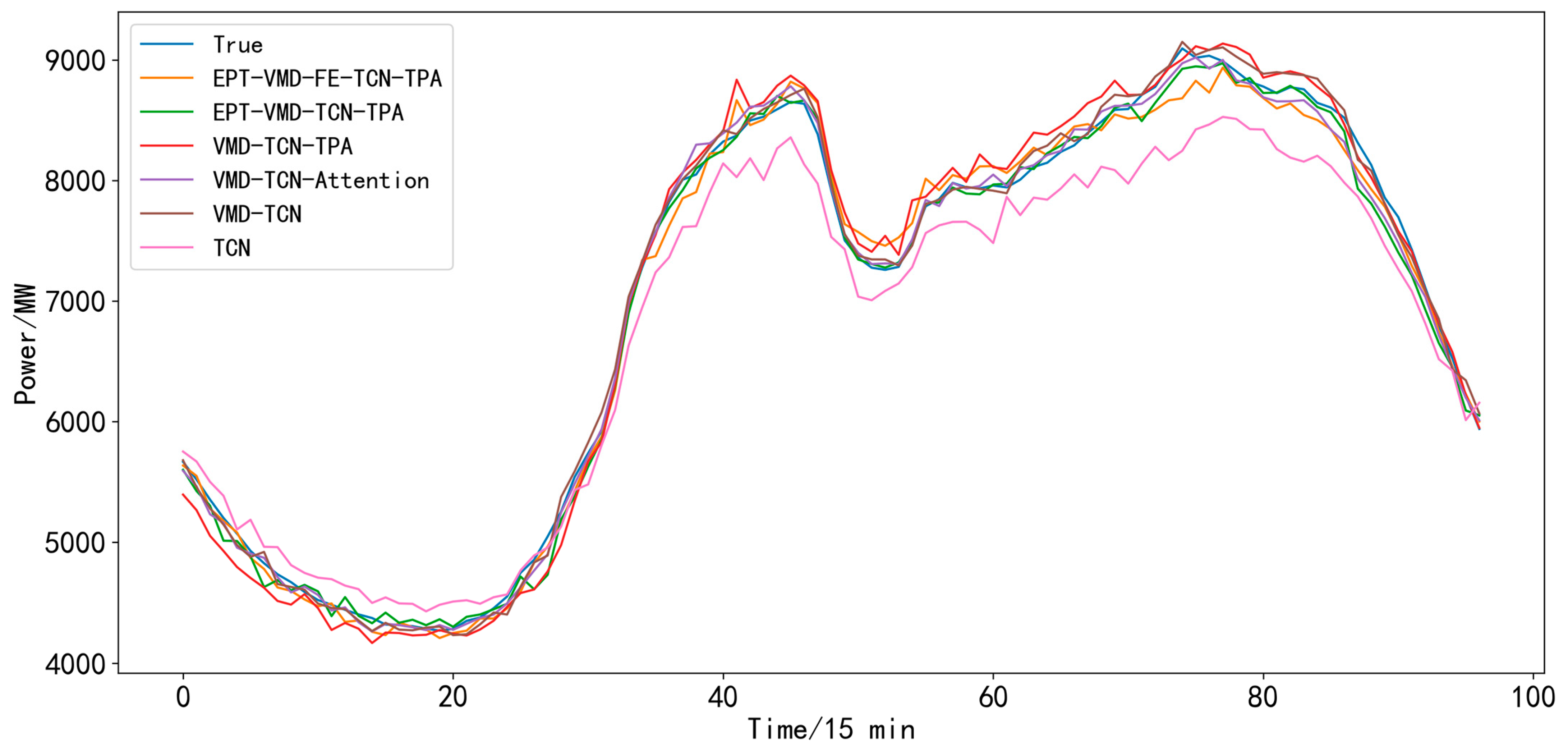
The prediction effects of each of the above comparison models on the test set are shown in Figure 17 (only one day is shown), and the prediction error evaluation index data and fit effect data of each model are shown in

Table 8. Area 1 ablation model evaluation indicators.

Model	MAPE (%)	RMSE (MW)	MAE (MW)	R2	Time (s)
TCN	2.84	247.9006	181.3514	0.9774	34.040
VMD-TCN	2.59	187.9851	147.2761	0.9870	390.934
VMD-TCN-Attention	1.58	133.4030	102.7410	0.9934	383.140
VMD-TCN-TPA	1.54	122.1089	98.6245	0.9945	427.891
EPT-VMD-TCN-TPA	1.25	110.2692	82.3180	0.9955	443.232
EPT-VMD-FE-TCN-TPA	1.86	168.9959	121.6994	0.9895	296.137

.

As can be seen in Table 8, the EPT-VMD-TCN-TPA forecasting model proposed in this paper has the smallest MAPE, RMSE, and MAE compared with other comparative models, which are 1.25%, 110.2692 MW, and 82.3180 MW, respectively. Furthermore, the EPT-VMD-TCN-TPA model has the highest R2 value, 0.9955. These evaluation indexes reflect that the EPT-VMD-TCN-TPA forecasting model proposed in this paper can achieve accurate forecasting results for short-term load forecasting. The TCN model, as the most basic model, has the worst forecasting effect and takes the shortest time. From the TCN, VMD-TCN, VMD-TCN-Attention, and VMD-TCN-TPA until the EPT-VMD-TCN-TPA model, its prediction accuracy improves step by step, which also indicates that each step in the EPT-VMD-TCN-TPA model and the combination together will be beneficial for the improvement of prediction precision. Compared with the TCN model, the MAPE, RMSE, and MAE of the EPT-VMD-TCN-TPA model are reduced by 55.99%, 55.52%, and 54.61%, respectively, which indicates that the EPT-VMD-TCN-TPA model has a high predictive fine-reading. As shown in Figure 17, the EPT-VMD-TCN-TPA model has a relatively accurate prediction effect both in the wave peak and the trough. In terms of model running efficiency, the EPT-VMD-TCN-TPA model proposed in this paper takes 443.232 s, which is the longest time among all the models. This is because the decomposition of the load using EPT and VMD makes the number of prediction components increase, which leads to the long running time of the model. In real life, the accuracy of the prediction results will be given priority, and with the continuous upgrading of hardware and the application of parallel computing, the running efficiency of the EPT-VMD-TCN-TPA model proposed in this paper will not be a problem.

As shown in Table 8, the EPT-VMD-FE-TCN-TPA recombination model, which uses the sample entropy (FE) to evaluate the complexity of the IMF, has better prediction results compared to TCN and VMD-TCN. The EPT-VMD-FE-TCN-TPA recombination model has lower prediction precision compared to the EPT-VMD-TCN-TPA model, although operational efficiency is improved due to the reduced computational size. In the next step, we will consider how to use FE more rationally to evaluate the complexity of IMF so that the EPT-VMD-FE-TCN-TPA reorganization model can be run more efficiently with guaranteed accuracy.

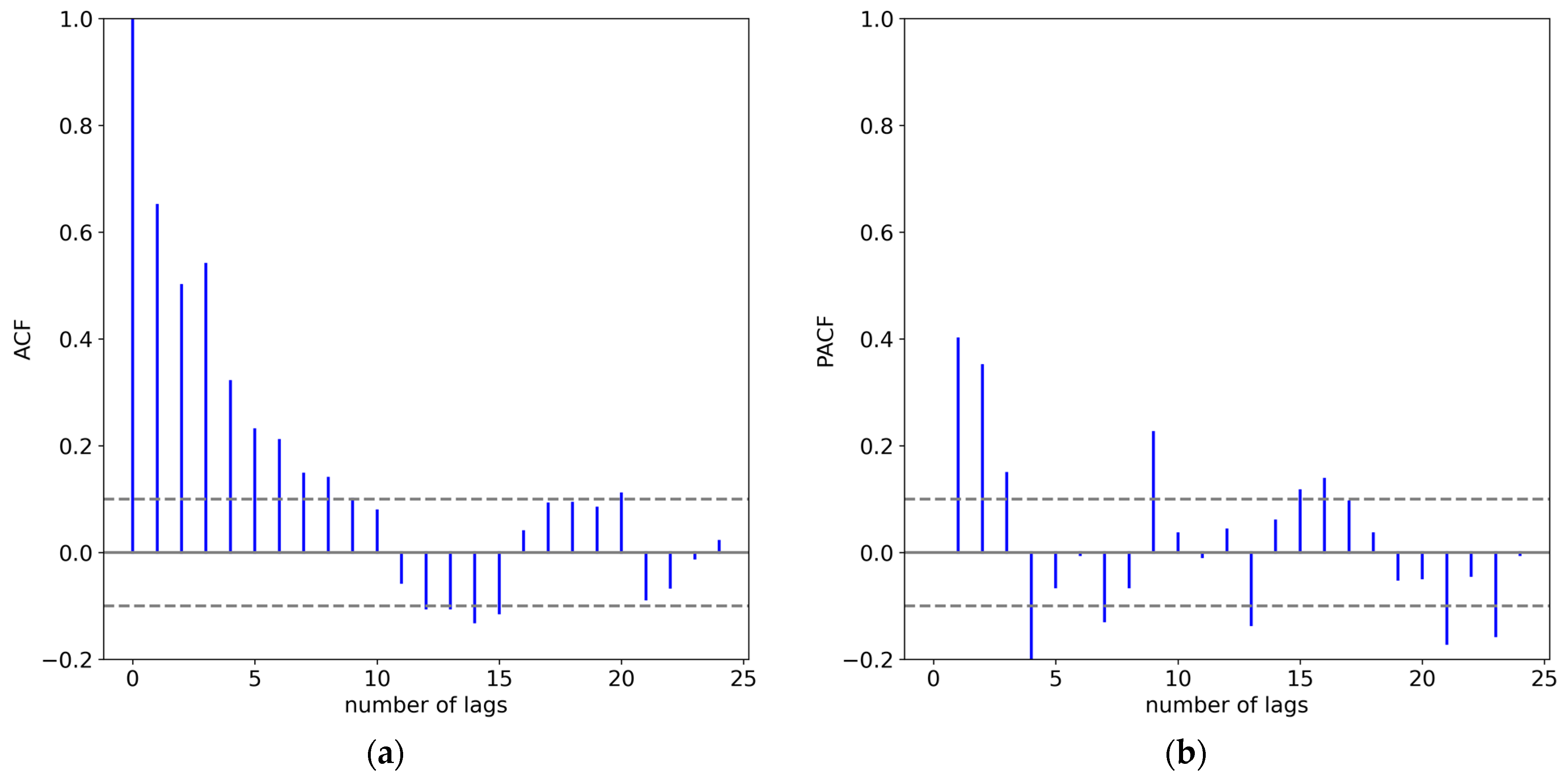
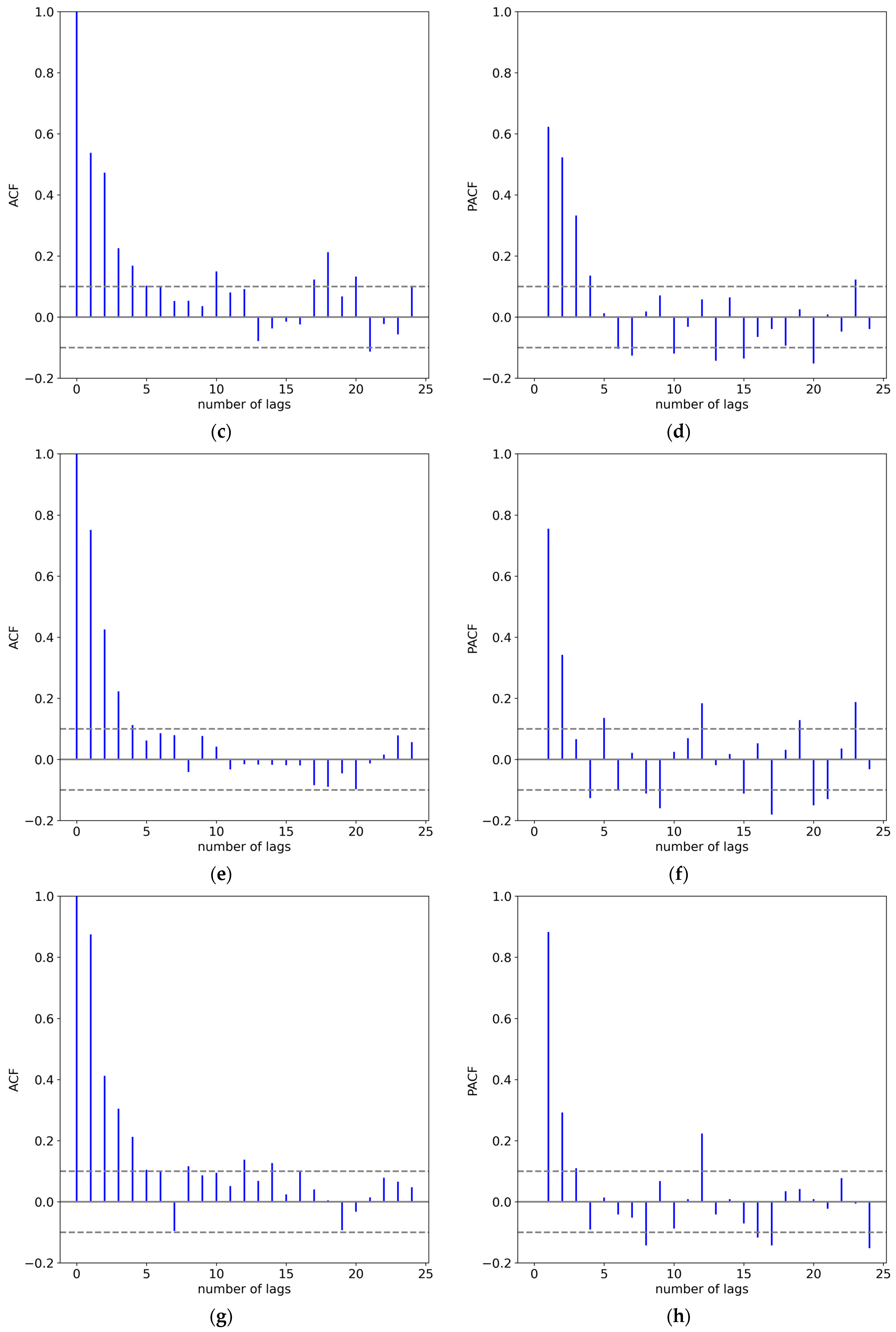
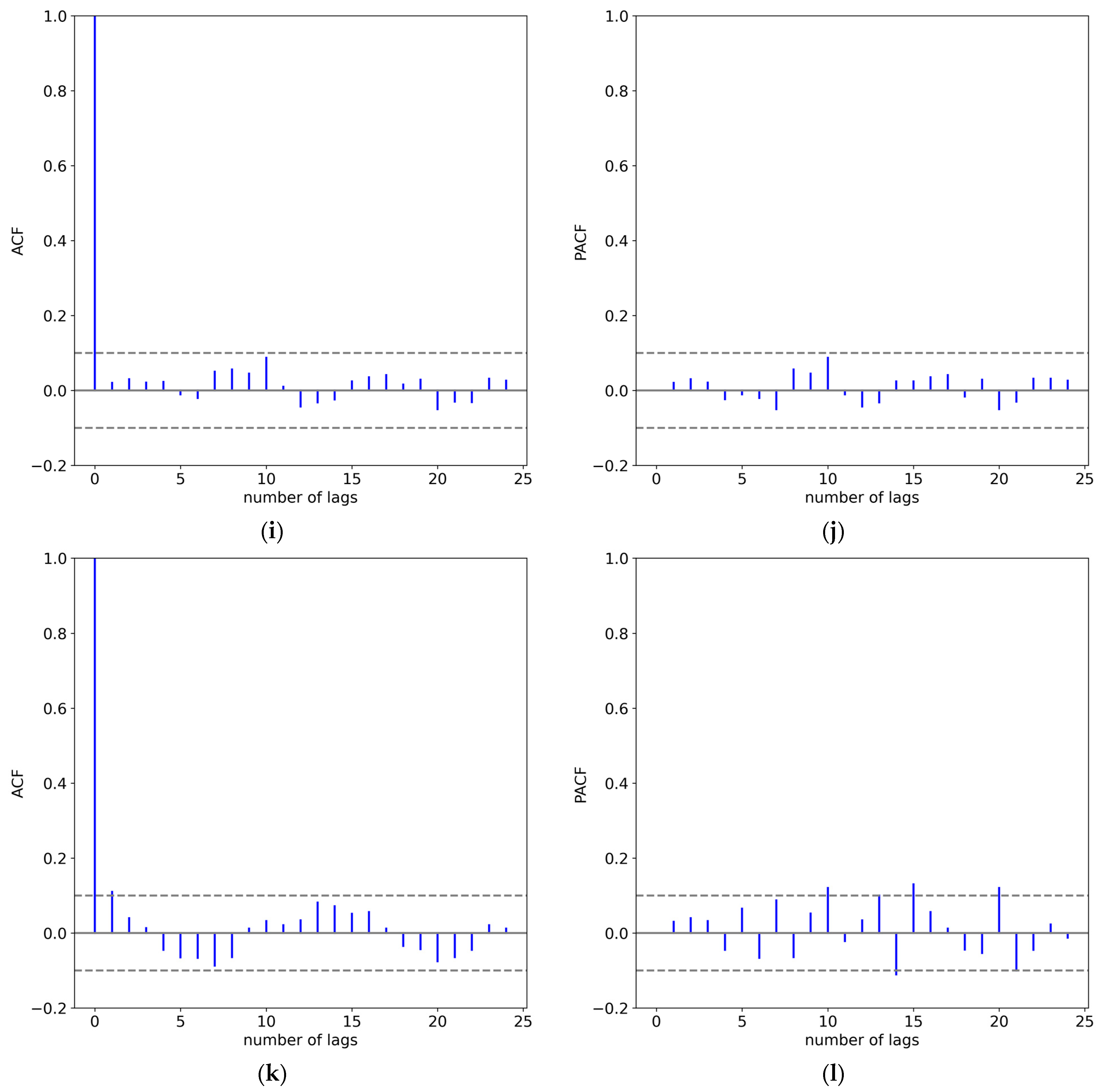
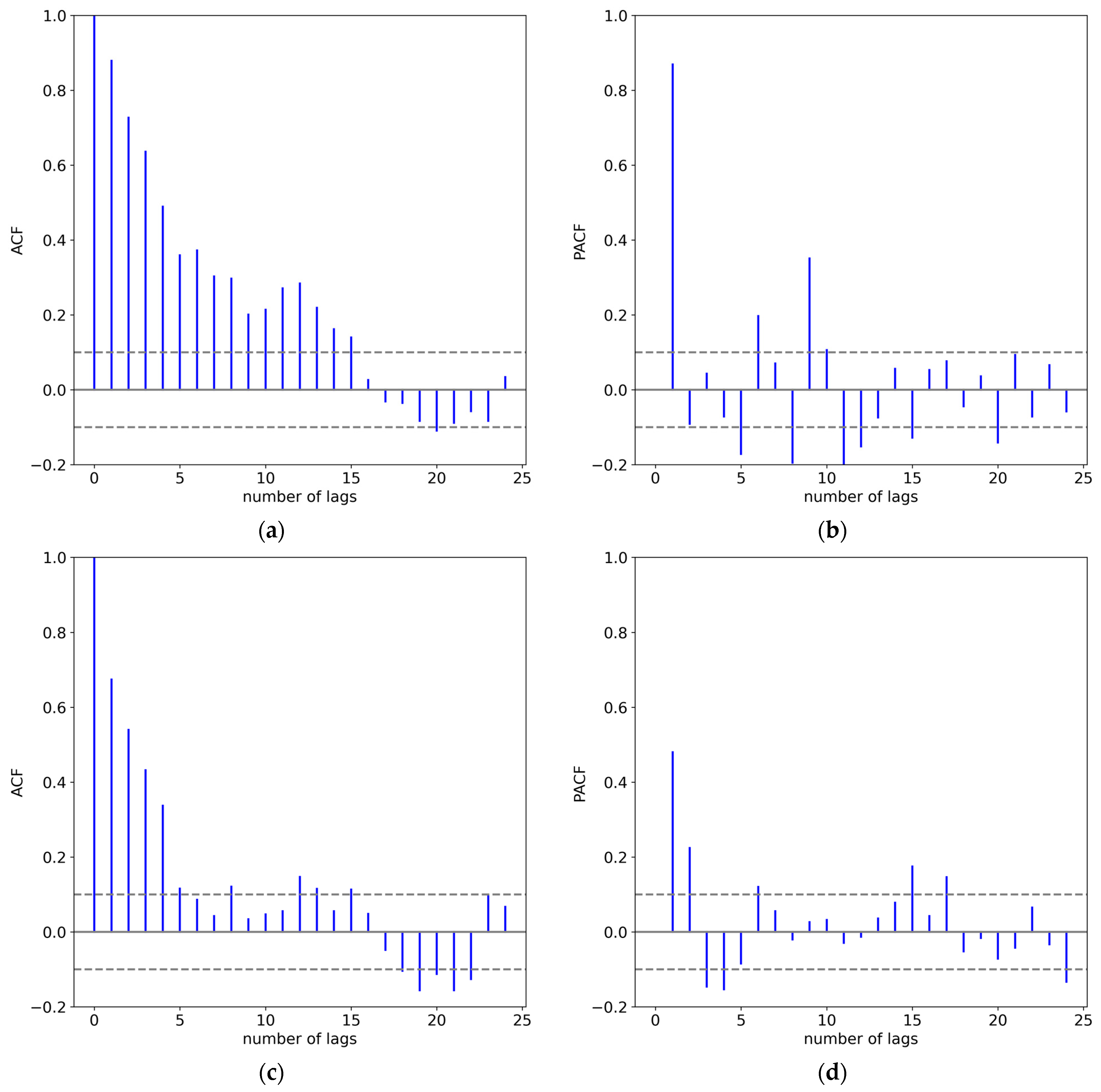
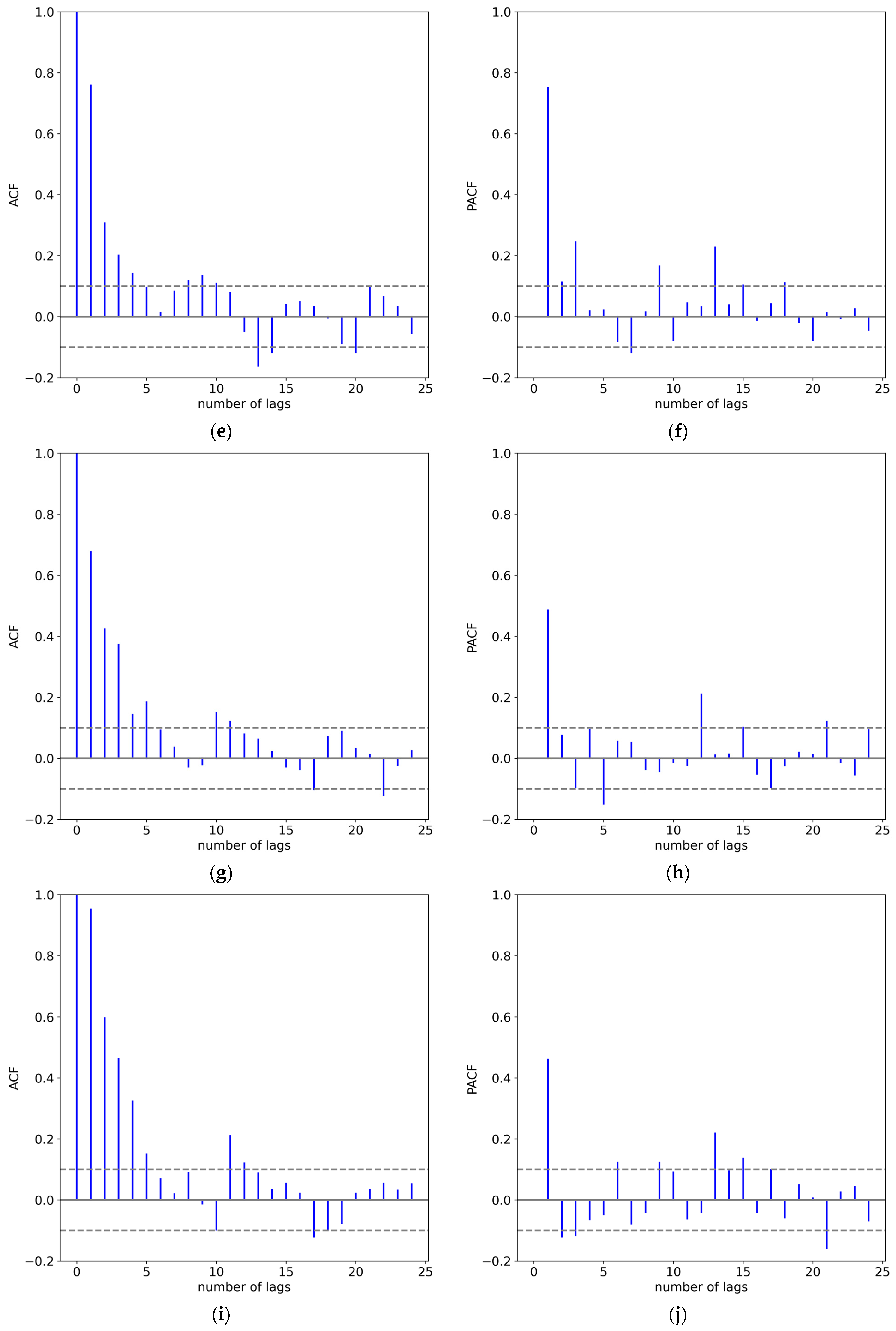
The autocorrelation function (ACF) and partial autocorrelation function (PACF) of the final residuals of all models in Table 8 are shown in Figure 18. In Figure 18, it can be seen that the final residuals in the EPT-VMD-TCN-TPA short-term load prediction model and the EPT-VMD-FE-TCN-TPA recombination model proposed in this paper have been whitened, which indicates the validity of these two models proposed in this paper.

In order to verify the performance of the models proposed in this paper with the ablation comparison models in Table 8, we performed DM tests for each pair of models. The results of the DM tests are listed in

Table 9. DM test value table.

Model	TCN	VMD-TCN	VMD-TCN-Attention	VMD-TCN-TPA	EPT-VMD-TCN-TPA	EPT-VMD-FE-TCN-TPA
TCN	nan	0.0112 (−2.538)	0.0007 (−3.386)	0.0003 (−3.590)	0.0002 (−3.765)	0.0110 (−2.543)
VMD-TCN	0.0112 (2.538)	nan	0.0877 (−1.708)	0.0472 (−1.985)	0.0260 (−2.227)	0.5255 (−0.635)
VMD-TCN-Attention	0.0007 (3.386)	0.0877 (1.708)	nan	0.0083 (−2.642)	0.0000 (−8.145)	0.0106 (2.555)
VMD-TCN-TPA	0.0003 (3.590)	0.0472 (1.985)	0.0083 (2.642)	nan	0.0066 (−2.716)	0.0021 (3.073)
EPT-VMD-TCN-TPA	0.0002 (3.765)	0.0260 (2.227)	0.0000 (8.145)	0.0066 (2.716)	nan	0.0001 (4.018)
EPT-VMD-FE-TCN-TPA	0.0110 (2.543)	0.5255 (0.635)	0.0106 (−2.555)	0.0021 (−3.073)	0.0001 (−4.018)	nan

.

In Table 9, the DM test uses MSE as a metric. The original hypothesis H in the DM test is that the column model and the row model have the same effect. The alternative hypothesis H0 in the DM test is a column model and a row model with different effects. The experimental results are p-values outside the parentheses and DM statistics inside the parentheses. If the p-value > 0.05, the effect of the row model is the same as that of the column model in the comparison; if p < 0.05 and the DM value is positive, it means that the effect of the row model is better than that of the column model with which it is compared; and if p < 0.05 and the DM value is negative, it means that the effect of the column model is better than that of the row model with which it is compared. As can be seen in the table, the experimental effect of our proposed EPT-VMD-TCN-TPA short-term load prediction model is better than other ablation comparison experiments. The experimental results of the recombinant EPT-VMD-FE-TCN-TPA short-term load prediction model proposed in this paper are statistically inferior to the EPT-VMD-TCN-TPA model proposed in this paper. However, when combined with the results of the classical experimental comparison models in DM inspection, the recombinant model can still achieve good prediction results.

4.5. Classic Experiments

To verify the accuracy of the prediction model proposed in this paper, we compared SVR, LSTM, CNN-LSTM, LSTM-Attention, BiLSTM, and the EPT-VMD-TCN-TPA prediction model in this paper. We will illustrate that our proposed prediction models are more accurate by the evaluation metrics of the prediction results. These comparative models are related as follows:

(1)

SVR prediction model: Support vector regression prediction model.

(2)

LSTM prediction model [23]: A typical recurrent neural network with memory function and gate structure, which can effectively solve the problem of gradient disappearance and gradient explosion due to excessive sequence length in RNN models.

(3)

CNN-LSTM prediction model [50]: By combining CNN and LSTM models, it enables the model to extract features inside the data through the convolution operation of the CNN, while using LSTM models to predict changes in the time series.

(4)

LSTM-Attention prediction model [22]: This model introduces the attention mechanism based on the LSTM model. The attention mechanism assigns more weight to important features, thus strengthening the connection between the whole and the local, and improving the prediction accuracy.

(5)

BiLSTM prediction model [25]: This model is improved on the basis of the LSTM model. Both forward and backward sequence information inputs are available to fully extract the information from the load data.

(6)

EPT-VMD-TCN-TPA prediction model: Our proposed final model.

(7)

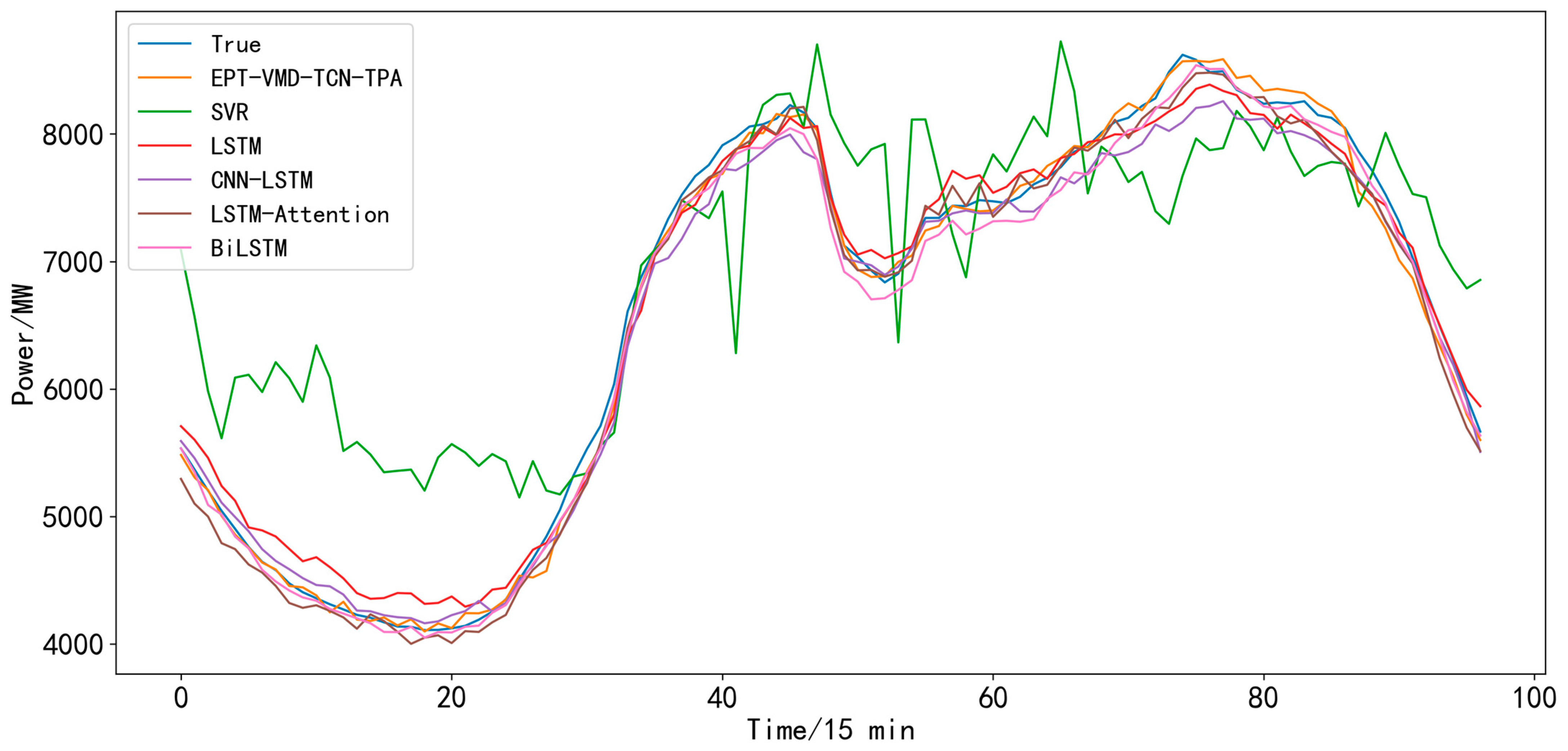
The prediction effects of the EPT-VMD-TCN-TPA model and the above comparison model on the test set are shown in Figure 19 (only one day is shown), and the prediction error evaluation index data and fit effect data for each model are shown in

Table 10. Classical model evaluation indicators for Area 1.

Model	MAPE (%)	RMSE (MW)	MAE (MW)	R2	Time (s)
SVR	16.07	1309.0193	1022.1499	0.3689	11.666
LSTM	3.48	320.5932	222.2477	0.9621	39.803
CNN-LSTM	3.27	291.7813	203.8683	0.9686	45.583
LSTM-Attention	3.82	379.4524	229.1554	0.9470	57.898
BiLSTM	3.15	273.6259	200.7860	0.9724	93.655
EPT-VMD-TCN-TPA	1.25	110.2692	82.3180	0.9955	443.232

.

As can be seen in Table 10, our proposed EPT-VMD-TCN-TPA model has the lowest MAPE, RMSE, and MAE compared to other comparative models, with 1.25%, 110.2692 MW, and 82.3180 MW, respectively, and the largest fitting index R² of 0.9955. It is thus clear that the EPT-VMD-TCN-TPA model can predict the load accurately. Compared with the common LSTM model, the MAPE, RMSE, and MAE of the EPT-VMD-TCN-TPA model are reduced by 64.08%, 65.60%, and 62.96%, respectively, which indicates that the EPT-VMD-TCN-TPA model has a high prediction accuracy. As can be seen in Figure 19, the EPT-VMD-TCN-TPA model has the best prediction effect and the best accuracy for the wave and trough prediction results. Of course, the running time of the EPT-VMD-TCN-TPA model is still the longest, but with the upgrade of hardware devices and parallel computing, the model’s running efficiency will be improved significantly.

The autocorrelation function (ACF) and partial autocorrelation function (PACF) for the final residuals of all the models in Table 10 are shown in Figure 20. It can be seen in Figure 20 that the classical comparative model has an autocorrelation structure, indicating that it does not predict well. In the previous Figure 18i,j, it is known that the EPT-VMD-TCN-TPA model proposed in this paper has been whitened, which further illustrates the best performance of the model in this paper.

In order to verify the performance of the models proposed in this paper with the classical comparison models in Table 10, we performed DM tests for each pair of models. The results of the DM tests are listed in

Table 11. DM test value table.

Model	SVR	LSTM	CNN-LSTM	LSTM-Attention	BiLSTM	EPT-VMD-TCN-TPA	EPT-VMD-FE-TCN-TPA
SVR	nan	0.0000 (−5.779)	0.0000 (−5.828)	0.0000 (−6.444)	0.0000 (−5.502)	0.0000 (−5.649)	0.0000 (−5.603)
LSTM	0.0000 (5.779)	nan	0.0010 (−3.289)	0.3682 (0.899)	0.2256 (−1.212)	0.0018 (−3.127)	0.0082 (−2.644)
CNN-LSTM	0.0000 (5.828)	0.0010 (3.289)	nan	0.2191 (1.229)	0.6427 (−0.464)	0.0058 (−2.759)	0.0274 (−2.205)
LSTM-Attention	0.0000 (6.444)	0.3682 (−0.899)	0.2191 (−1.229)	nan	0.2869 (−1.065)	0.0087 (−2.821)	0.0179 (−2.608)
BiLSTM	0.0000 (5.502)	0.2256 (1.212)	0.6427 (0.464)	0.2869 (1.065)	nan	0.0000 (−4.811)	0.0003 (−3.587)
EPT-VMD-TCN-TPA	0.0000 (5.649)	0.0018 (3.127)	0.0058 (2.758)	0.0087 (2.821)	0.0000 (4.811)	nan	0.0001 (4.018)
EPT-VMD-FE-TCN-TPA	0.0000 (5.604)	0.0082 (2.644)	0.0275 (2.205)	0.0179 (2.608)	0.0003 (3.587)	0.0001 (−4.018)	nan

.

In Table 11, this DM test table (using the MSE metric) uses the original hypothesis H, which proposes that the column and row models have the same effect. The alternative hypothesis H0 proposes that the column and row models have different effects. The experimental results are p-values outside the parentheses and DM statistics inside the parentheses. If the p-value > 0.05, the effect of the row model is the same as that of the column model in the comparison; if p < 0.05 and the DM value is positive, it means that the effect of the row model is better than that of the column model with which it is compared; and if p < 0.05 and the DM value is negative, it means that the effect of the column model is better than that of the row model with which it is compared. In the table, we can see that the experimental effect of our proposed EPT-VMD-TCN-TPA short-term load prediction model is better than other classical comparison experiments, and the experimental effect of the recombinant EPT-VMD-FE-TCN-TPA short-term load prediction model proposed in this paper is also better than other classical comparison experiments, second only to the EPT-VMD-TCN-TPA model. The prediction effects of BiLSTM, LSTM, CNN-LSTM, and LSTM-Attention are not much different. The SVR has the worst effect in the comparison experiments.

From the comparison of the ablation experiments, as well as the classical experiments, it is clear that our proposed EPT-VMD-TCN-TPA model shows greater advantages in handling complex electric load forecasting data and improving forecasting accuracy. The next section will evaluate the robustness and applicability of the EPT-VMD-TCN-TPA model using the classical comparison experiments in Area 2.

5. Experimental Results in Area 2

In the previous section, we validated our proposed short-term load forecasting method based on the data from region 1 and obtained good experimental results. However, relying on only one dataset to validate the experiments may be subject to chance, so in order to verify the accuracy as well as the generalizability of our proposed model, we conducted experiments using the dataset of Area 2 provided by the 9th National Electrician Mathematical Modeling Competition in China. One of the EPT-VMD decomposition parts is described in Section 3.2. The ablation experimental result pairs of the EPT-VMD-TCN-TPA model proposed in this paper are shown in Figure 21. The error evaluation indexes and fitting effect data of each model are shown in

Table 12. Area 2 ablation model evaluation indicators.

Model	MAPE (%)	RMSE (MW)	MAE (MW)	R2	Time (s)
TCN	3.02	279.9281	207.6085	0.9681	31.759
VMD-TCN	1.68	147.2106	116.8644	0.9912	356.854
VMD-TCN-Attention	1.63	144.1170	110.6246	0.9915	379.672
VMD-TCN-TPA	1.60	140.2134	109.3452	0.9919	411.754
EPT-VMD-TCN-TPA	1.58	137.6182	107.2617	0.9923	424.006
EPT-VMD-FE-TCN-TPA	2.02	170.3671	135.1109	0.9882	243.455

. The classical comparison experimental results are shown in Figure 22 and the evaluation indexes of each model are shown in

Table 13. Area 2 evaluation indicators for each model.

Model	MAPE (%)	RMSE (MW)	MAE (MW)	R2	Time (s)
SVR	13.11	1103.4697	882.2721	0.5045	6.910
LSTM	3.64	355.7457	249.5678	0.9485	32.688
CNN-LSTM	3.26	294.3930	222.8188	0.9647	79.906
LSTM-Attention	3.85	383.7617	265.7952	0.9401	73.906
BiLSTM	2.64	254.9352	178.6009	0.9736	131.753
EPT-VMD-TCN-TPA	1.58	137.6182	107.2617	0.9923	424.006

.

As shown in Table 12 and Table 13 and Figure 21 and Figure 22, the MAPE, RMSE, and MAE of the EPT-VMD-TCN-TPA prediction model are 1.58%, 137.6182 MW, and 107.2617 MW, respectively. The R² reaches 0.9923. Compared with other models, our proposed EPT-VMD-TCN-TPA prediction model has the best prediction results. Therefore, it is evident that our proposed EPT-VMD-TCN-TPA model has some stability and scalability.

6. Conclusions

Accurate and effective power load forecasting is of great significance for the safe, economical, and stable operation of power grids. However, the complexity and non-smoothness of power load data bring difficulties to power load forecasting. Therefore, this paper proposes a combined decomposition (EPT-VMD) combined with TCN-TPA network forecasting for short-term power load forecasting, i.e., the EPT-VMD-TCN-TPA forecasting model. The method first extracts the trend component and residual fluctuation component of the original load series using EPT, and the trend component has obvious periodicity, which can improve the prediction precision reading. Secondly, the residual fluctuation components are decomposed into intrinsic mode function components with different center frequencies using VMD, and the ratio of the residual energy after decomposition is used to determine the number of decompositions k of VMD, which effectively avoids over-decomposition and under-decomposition. Using a network model with TCN-TPA for training and prediction of components, the TCN-TPA network can be better applied to multivariate time series prediction. Finally, the prediction results of each component are accumulated to obtain the predicted values of the final load. We also discuss the performance of the EPT-VMD-FE-TPA-TCN prediction model using FE.

To test the performance of the proposed EPT-VMD-TCN-TPA model, experiments were conducted on real datasets from two Areas provided by the 9th National Electrician Mathematical Modeling Competition in China. The predictive precision of the models was evaluated by MAE, MAPE, RMSE, and R², and the significance of the differences in model prediction performance was assessed using the DM test. The results show that our proposed method has better prediction accuracy than other methods. The MAPE of the EPT-VMD-TCN-TPA method proposed in this paper was 1.25% and 1.58% for the test results on two regions, respectively. Although the method proposed in this paper achieved good results, only meteorological data and load data were considered in this paper. Therefore, we suggest that more influencing factors, such as the date factor, electricity price, and social development level, should be considered in future studies. In addition, suitable optimization algorithms can be used to optimally select the model hyperparameters to produce more accurate prediction results.

References

1. Fallah, S.; Deo, R.; Shojafar, M.; Conti, M.; Shamshirband, S. Computational Intelligence Approaches for Energy Load Forecasting in Smart Energy Management Grids: State of the Art, Future Challenges, and Research Directions. Energies 2018, 11, 596. [Google Scholar] [CrossRef] [Green Version]
2. Li, J.; Luo, Y.; Wei, S. Long-Term Electricity Consumption Forecasting Method Based on System Dynamics under the Carbon-Neutral Target. Energy 2022, 244, 122572. [Google Scholar] [CrossRef]
3. Nti, I.K.; Teimeh, M.; Nyarko-Boateng, O.; Adekoya, A.F. Electricity Load Forecasting: A Systematic Review. J. Electr. Syst. Inf. Technol. 2020, 7, 13. [Google Scholar] [CrossRef]
4. Ahmad, T.; Zhang, H.; Yan, B. A Review on Renewable Energy and Electricity Requirement Forecasting Models for Smart Grid and Buildings. Sustain. Cities Soc. 2020, 55, 102052. [Google Scholar] [CrossRef]
5. Mishra, M.; Nayak, J.; Naik, B.; Abraham, A. Deep Learning in Electrical Utility Industry: A Comprehensive Review of a Decade of Research. Eng. Appl. Artif. Intell. 2020, 96, 104000. [Google Scholar] [CrossRef]
6. Kuster, C.; Rezgui, Y.; Mourshed, M. Electrical load forecasting models: A critical systematic review. Sustain. Cities Soc. 2017, 35, 257–270. [Google Scholar] [CrossRef]
7. Tan, F.L.; Zhang, J.; Ma, H.Z. Combined forecasting method of power load based on trend change division. J. N. China Electr. Power Univ. 2020, 47, 17–24. [Google Scholar]
8. Christiaanse, W. Short-Term Load Forecasting Using General Exponential Smoothing. IEEE Trans. Power Appar. Syst. 1971, PAS-90, 900–911. [Google Scholar] [CrossRef]
9. Chen, P.Y.; Fang, Y.J. Short-term load forecasting of power system for holiday point-by-point growth rate based on Kalman filtering. Eng. J. Wuhan Univ. 2020, 53, 139–144. [Google Scholar]
10. Munkhammar, J.; van der Meer, D.; Widén, J. Very Short Term Load Forecasting of Residential Electricity Consumption Using the Markov-Chain Mixture Distribution (MCM) Model. Appl. Energy 2021, 282, 116180. [Google Scholar] [CrossRef]
11. Wu, F.; Cattani, C.; Song, W.; Zio, E. Fractional ARIMA with an Improved Cuckoo Search Optimization for the Efficient Short-Term Power Load Forecasting. Alex. Eng. J. 2020, 59, 3111–3118. [Google Scholar] [CrossRef]
12. Duan, L.; Niu, D.; Gu, Z. Long and medium term power load forecasting with multi-level recursive regression analysis. In Proceedings of the 2008 Second International Symposium on Intelligent Information Technology Application, Shanghai, China, 20–22 December 2008; pp. 514–518. [Google Scholar]
13. Ceperic, E.; Ceperic, V.; Baric, A. A Strategy for Short-Term Load Forecasting by Support Vector Regression Machines. IEEE Trans. Power Syst. 2013, 28, 4356–4364. [Google Scholar] [CrossRef]
14. Hu, Y.; Li, J.; Hong, M.; Ren, J.; Lin, R.; Liu, Y.; Liu, M.; Man, Y. Short Term Electric Load Forecasting Model and Its Verification for Process Industrial Enterprises Based on Hybrid GA-PSO-BPNN Algorithm—A Case Study of Papermaking Process. Energy 2019, 170, 1215–1227. [Google Scholar] [CrossRef]
15. Kuhba, H.; Al-Tamemi, H.A.H. Power system short-term load forecasting using artificial neural networks. Int. J. Eng. Dev. Res. 2016, 4, 78–87. [Google Scholar]
16. Imani, M. Electrical Load-Temperature CNN for Residential Load Forecasting. Energy 2021, 227, 120480. [Google Scholar] [CrossRef]
17. Motepe, S.; Hasan, A.N.; Twala, B.; Stopforth, R. Power Distribution Networks Load Forecasting Using Deep Belief Networks: The South African Case. In Proceedings of the 2019 IEEE Jordan International Joint Conference on Electrical Engineering and Information Technology (JEEIT), Amman, Jordan, 9–11 April 2019; pp. 507–512. [Google Scholar]
18. Wang, C.; Huang, S.; Wang, S.; Ma, Y.; Ma, J.; Ding, J. Short term load forecasting based on vmd-dnn. In Proceedings of the 2019 IEEE 8th International Conference on Advanced Power System Automation and Protection (APAP), Online, 21–24 October 2019; pp. 1045–1048. [Google Scholar]
19. Zhang, B.; Wu, J.-L.; Chang, P.-C. A Multiple Time Series-Based Recurrent Neural Network for Short-Term Load Forecasting. Soft Comput. 2018, 22, 4099–4112. [Google Scholar] [CrossRef]
20. Hochreiter, S.; Schmidhuber, J. Long short-term memory. Neural Comput. 1997, 9, 1735–1780. [Google Scholar] [CrossRef] [PubMed]
21. Muzaffar, S.; Afshari, A. Short-Term Load Forecasts Using LSTM Networks. Energy Procedia 2019, 158, 2922–2927. [Google Scholar] [CrossRef]
22. Lin, J.; Ma, J.; Zhu, J.; Cui, Y. Short-Term Load Forecasting Based on LSTM Networks Considering Attention Mechanism. Int. J. Electr. Power Energy Syst. 2022, 137, 107818. [Google Scholar] [CrossRef]
23. Kong, W.; Dong, Z.Y.; Jia, Y.; Hill, D.J.; Xu, Y.; Zhang, Y. Short-Term Residential Load Forecasting Based on LSTM Recurrent Neural Network. IEEE Trans. Smart Grid 2019, 10, 841–851. [Google Scholar] [CrossRef]
24. Gao, X.; Li, X.; Zhao, B.; Ji, W.; Jing, X.; He, Y. Short-Term Electricity Load Forecasting Model Based on EMD-GRU with Feature Selection. Energies 2019, 12, 1140. [Google Scholar] [CrossRef] [Green Version]
25. Yan, L.; Zhang, H. A Variant Model Based on BiLSTM for Electricity Load Prediction. In Proceedings of the 2021 IEEE International Conference on Power, Intelligent Computing and Systems (ICPICS), Shenyang, China, 29 July 2021; pp. 404–411. [Google Scholar]
26. Niu, D.; Yu, M.; Sun, L.; Gao, T.; Wang, K. Short-Term Multi-Energy Load Forecasting for Integrated Energy Systems Based on CNN-BiGRU Optimized by Attention Mechanism. Appl. Energy 2022, 313, 118801. [Google Scholar] [CrossRef]
27. Song, J.; Xue, G.; Pan, X.; Ma, Y.; Li, H. Hourly Heat Load Prediction Model Based on Temporal Convolutional Neural Network. IEEE Access 2020, 8, 16726–16741. [Google Scholar] [CrossRef]
28. Wang, Y.; Chen, J.; Chen, X.; Zeng, X.; Kong, Y.; Sun, S.; Guo, Y.; Liu, Y. Short-Term Load Forecasting for Industrial Customers Based on TCN-LightGBM. IEEE Trans. Power Syst. 2021, 36, 1984–1997. [Google Scholar] [CrossRef]
29. Tang, X.; Chen, H.; Xiang, W.; Yang, J.; Zou, M. Short-Term Load Forecasting Using Channel and Temporal Attention Based Temporal Convolutional Network. Electr. Power Syst. Res. 2022, 205, 107761. [Google Scholar] [CrossRef]
30. Shah, I.; Jan, F.; Ali, S. Functional Data Approach for Short-Term Electricity Demand Forecasting. Math. Probl. Eng. 2022, 2022, 6709779. [Google Scholar] [CrossRef]
31. Shah, I.; Iftikhar, H.; Ali, S. Modeling and Forecasting Electricity Demand and Prices: A Comparison of Alternative Approaches. J. Math. 2022, 2022, 3581037. [Google Scholar] [CrossRef]
32. Shah, I.; Iftikhar, H.; Ali, S.; Wang, D. Short-Term Electricity Demand Forecasting Using ComponentsEstimation Technique. Energies 2019, 12, 2532. [Google Scholar] [CrossRef] [Green Version]
33. Li, B.; Zhang, J.; He, Y.; Wang, Y. Short-Term Load-Forecasting Method Based on Wavelet Decomposition with Second-Order Gray Neural Network Model Combined with ADF Test. IEEE Access 2017, 5, 16324–16331. [Google Scholar] [CrossRef]
34. Meng, Z.; Xie, Y.; Sun, J. Short-Term Load Forecasting Using Neural Attention Model Based on EMD. Electr. Eng. 2022, 104, 1857–1866. [Google Scholar] [CrossRef]
35. Dong, P.; Bin, X.; Jun, M.; Qian, D.; Jinjin, D.; Jinjin, Z.; Qian, Z. Short-Term Load Forecasting Based on EEMD-Approximate Entropy and ELM. In Proceedings of the 2019 IEEE Sustainable Power and Energy Conference (iSPEC), Beijing, China, 4–7 November 2019; pp. 1772–1775. [Google Scholar]
36. Zhang, Z.; Hong, W.-C.; Li, J. Electric Load Forecasting by Hybrid Self-Recurrent Support Vector Regression Model with Variational Mode Decomposition and Improved Cuckoo Search Algorithm. IEEE Access 2020, 8, 14642–14658. [Google Scholar] [CrossRef]
37. Yuan, F.; Che, J. An Ensemble Multi-Step M-RMLSSVR Model Based on VMD and Two-Group Strategy for Day-Ahead Short-Term Load Forecasting. Knowl. Based Syst. 2022, 252, 109440. [Google Scholar] [CrossRef]
38. Cai, C.; Li, Y.; Su, Z.; Zhu, T.; He, Y. Short-Term Electrical Load Forecasting Based on VMD and GRU-TCN Hybrid Network. Appl. Sci. 2022, 12, 6647. [Google Scholar] [CrossRef]
39. Kim, D.; Choi, G.; Oh, H.-S. Ensemble Patch Transformation: A Flexible Framework for Decomposition and Filtering of Signal. EURASIP J. Adv. Signal Process. 2020, 2020, 30. [Google Scholar] [CrossRef]
40. Heydari, A.; Keynia, F.; Garcia, D.A.; De Santoli, L. Mid-Term Load Power Forecasting Considering Environment Emission Using a Hybrid Intelligent Approach. In Proceedings of the 2018 5th International Symposium on Environment-Friendly Energies and Applications (EFEA), Rome, Italy, 24–26 September 2018; pp. 1–5. [Google Scholar]
41. Jiang, P.; Nie, Y.; Wang, J.; Huang, X. Multivariable Short-Term Electricity Price Forecasting Using Artificial Intelligence and Multi-Input Multi-Output Scheme. Energy Econ. 2023, 117, 106471. [Google Scholar] [CrossRef]
42. Sekhar, C.; Dahiya, R. Robust Framework Based on Hybrid Deep Learning Approach for Short Term Load Forecasting of Building Electricity Demand. Energy 2023, 268, 126660. [Google Scholar] [CrossRef]
43. Heydari, A.; Majidi Nezhad, M.; Pirshayan, E.; Astiaso Garcia, D.; Keynia, F.; De Santoli, L. Short-Term Electricity Price and Load Forecasting in Isolated Power Grids Based on Composite Neural Network and Gravitational Search Optimization Algorithm. Appl. Energy 2020, 277, 115503. [Google Scholar] [CrossRef]
44. Dragomiretskiy, K.; Zosso, D. Variational mode decomposition. IEEE Trans. Signal Process. 2013, 62, 531–544. [Google Scholar] [CrossRef]
45. Chen, W.; Wang, Z.; Xie, H.; Yu, W. Characterization of Surface EMG Signal Based on Fuzzy Entropy. IEEE Trans. Neural Syst. Rehabil. Eng. 2007, 15, 266–272. [Google Scholar] [CrossRef]
46. Shih, S.-Y.; Sun, F.-K.; Lee, H. Temporal Pattern Attention for Multivariate Time Series Forecasting. Mach. Learn. 2019, 108, 1421–1441. [Google Scholar] [CrossRef] [Green Version]
47. Liu, Y.; Yang, C.; Huang, K.; Gui, W. Non-Ferrous Metals Price Forecasting Based on Variational Mode Decomposition and LSTM Network. Knowl. Based Syst. 2020, 188, 105006. [Google Scholar] [CrossRef]
48. Tran, T.N. Grid Search of Convolutional Neural Network model in the case of load forecasting. Arch. Electr. Eng. 2021, 2022, 3581037. [Google Scholar]
49. Shah, I.; Iftikhar, H.; Ali, S. Modeling and Forecasting Medium-Term Electricity Consumption Using Component Estimation Technique. Forecasting 2020, 2, 163–179. [Google Scholar] [CrossRef]
50. Rafi, S.H.; Nahid-Al-Masood; Deeba, S.R.; Hossain, E. A Short-Term Load Forecasting Method Using Integrated CNN and LSTM Network. IEEE Access 2021, 9, 32436–32448. [Google Scholar] [CrossRef]
Figure 1. Classification chart of load forecasting methods.
Applsci 13 04462 g001
Figure 2. The general flow of power load forecasting.
Applsci 13 04462 g002
Figure 3. VMD calculation process.
Applsci 13 04462 g003
Figure 4. Dilated causal convolution.
Applsci 13 04462 g004
Figure 5. Residual blocks.
Applsci 13 04462 g005
Figure 6. The TPA mechanism.
Applsci 13 04462 g006
Figure 7. The structural framework of the EPT-VMD-TCN-TPA model.
Applsci 13 04462 g007
Figure 8. Annual load of Area 1.
Applsci 13 04462 g008
Figure 9. Load trend chart for four consecutive weeks for Area 1.
Applsci 13 04462 g009
Figure 10. Area 1 EPT decomposition results.
Applsci 13 04462 g010
Figure 11. Area 2 EPT decomposition results.
Applsci 13 04462 g011
Figure 12. Area 1 VMD results.
Applsci 13 04462 g012
Figure 13. Area 2 VMD results.
Applsci 13 04462 g013
Figure 14. Fuzzy entropy of each IMF.
Applsci 13 04462 g014
Figure 15. FE reorganization results for Area 1.
Applsci 13 04462 g015
Figure 16. A flowchart of EPT-VMD-TCN-TPA model.
Applsci 13 04462 g016
Figure 17. Area 1 ablation experiment prediction results.
Applsci 13 04462 g017
Figure 18. ACF and PACF plots of TCN (a,b), VMD-TCN (c,d), VMD-TCN-Attention (e,f), VMD-TCN-TPA (g,h), EPT-VMD-TCN-TPA (i,j), EPT-VMD-FE-TCN-TPA (k,l).
Applsci 13 04462 g018aApplsci 13 04462 g018bApplsci 13 04462 g018c
Figure 19. Area 1 classical model prediction results.
Applsci 13 04462 g019
Figure 20. ACF and PACF plots of SVR (a,b), LSTM (c,d), CNN-LSTM (e,f), LSTM-Attention (g,h), BiLSTM (i,j).
Applsci 13 04462 g020aApplsci 13 04462 g020b
Figure 21. Area 2 ablation experiment prediction results.
Applsci 13 04462 g021
Figure 22. Area 2 prediction results for each model.
Applsci 13 04462 g022