The Evolution of the Corrosion Mechanism of Structural Steel Exposed to the Urban Industrial Atmosphere for Seven Years

Abstract

The corrosion mechanism and characteristics of steel in typical atmospheric environments directly affect the rationality of corrosion protection methods. This study investigates the corrosion evolution law of Q235 steel that has been exposed to the urban industrial atmosphere for seven years. The mass loss is used for corrosion dynamics analysis. The rust layers have been characterized by SEM, EDS, and XRD. Finally, the corrosion mechanism was analyzed through a combination of electrochemical methods, corrosion kinetics, and rust layer characteristics. The mass loss results indicate that a two-stage corrosion power function law can still effectively describe the corrosion rate of a seven-year exposure that complies with the power function law. The short-term corrosion results fail to fully reflect the corrosion performance of Q235 steel. The typical morphological structures of γ-FeOOH and α-FeOOH are identified, and the rust layers change from a loose and flat form to a granular and, finally, compact into a smooth surface. The crystalline phases of the rust layers include α-FeOOH, γ-FeOOH, Fe₃O₄/γ-Fe₂O₃ and α-Fe₂O₃. Corrosion products in the initial period are mainly γ-FeOOH, followed by α-FeOOH, and a small amount of Fe₃O₄/γ-Fe₂O₃. With the increase in exposure time, α-FeOOH and Fe₃O₄/γ-Fe₂O₃ in the rust layer increase. SO₂ and Fe₃O₄/γ-Fe₂O₃ are the primary factors accelerating steel corrosion. During the first three years of atmospheric corrosion, the primary corrosion mechanism was governed by the acid cycle reaction mechanism. However, from the fifth year of atmospheric corrosion, oxygen-absorbing corrosion began to gradually dominate, specifically oxygen-absorbing corrosion.

1. Introduction

Atmospheric corrosion is a gradual process that involves electrochemical reactions between the chemical compositions of materials and the atmosphere, resulting in surface morphology changes, a reduction in mass (thickness), and degradation of performance. Atmospheric corrosion of metals is extremely common in nature, since 80% of metal components are used in atmospheric environments [1]. Economic losses caused by atmospheric corrosion exceed the total losses caused by other conditions [2,3]. Steel is the most widely used metal in atmospheric environments due to its excellent mechanical properties [4]. However, atmospheric corrosion of steel can lead to the loss of cross-sectional structural members, compromising the bearing capacity of steel structures. Under the coupling effect of load and corrosion, the safety and reliability of steel structures can be severely compromised, and even catastrophic accidents can occur. About 25–40% of corrosion losses can be avoided if effective anti-corrosion measures are taken [5,6,7]. Therefore, it is necessary to investigate the behaviors and characteristics of steel corrosion, accumulate steel corrosion data, conduct corrosion evaluation, and predict steel lifespan to establish a foundation for reasonable material selection and the design of anti-corrosion schemes. Such studies have important application value for reducing the rate of atmospheric corrosion of steel, extending its service life, and minimizing the various losses caused by corrosion.

To date, a significant number of atmospheric corrosion studies have mainly focused on the initial stages of corrosion behaviors [8,9,10,11,12], as well as the impact of pollutants such as SO₂ and Cl⁻ during short-term (0.5–3 years) atmospheric exposure [13,14,15,16,17,18] and deposited atmospheric particulates [11] on the corrosion rate. Environmental parameters such as temperature, relative humidity [18,19], and time-of-wetness [20,21] were also explored to reveal their effects on corrosion rates. Some studies have established corrosion kinetic models for both short-term (3 years) and long-term (16 years) atmospheric exposures [22,23,24,25,26,27]. Models that predict corrosion rates have also been constructed [28,29]. In addition, the evaluation of corrosion products produced after atmospheric exposure is beneficial for understanding the corrosion behaviors of different steel materials, environmental conditions, and exposure time [30]. A number of studies have investigated the characteristics of corrosion products under short-term (a few months to a year) [31,32,33,34,35,36] and long-term [4,30] atmospheric exposures. The extension of the service life of steel is affected by its type and chemical composition [37]. Small amounts of alloying elements, mainly Cu, Cr, Ni, Mo, and P, were added to carbon steel to improve corrosion resistance and explore corrosion mechanisms under short-term (2–3 years) atmospheric exposure [37,38,39,40,41] and the protection mechanisms of its corrosion products in short- and long-term atmospheric exposures [30,36,37,40,41,42,43,44,45,46,47,48,49].

The abovementioned research on corrosion behaviors has achieved fruitful results. However, most of them focus on the corrosion behavior of steel under different corrosion environments for a short-term period of no more than 3 years. The medium- and long-term research information is considerably less abundant. The longer the atmospheric exposure time, the more reliable the atmospheric corrosion parameters obtained. After 13 years of exposure in five Spanish atmospheres of different types (rural, urban, industrial, and marine), de la Fuente et al. [4] assessed the structure and morphology of corrosion product layers formed on mild steel (0.44% C, 0.40% Mn, 0.018% S, <0.22% P, <0.05% Si, <0.1% Cr, <0.1% Ni, <0.1% Mo, and <0.05% Cu, Bal. Fe (wt%)), and found that: (1) in all cases, the corrosion rate decreased with exposure time, stabilizing after the first 4–6 years of exposure; (2) the great compaction of the rust layers were formed in the rural and urban atmospheres; (3) hematite and ferrihydrite phases were formed in the industrial and marine atmospheres, respectively. Liang et al. [25,26] studied the corrosion dynamics of carbon steel (0.20% C, 0.60% Mn, 0.009% S, 0.015% P, 0.30% Si, 98.876% Fe (wt%)) and low alloy steel after 16 years of exposure in the typical environment of China and revealed that the development of atmospheric corrosion of steel followed the power function law and the corrosion in marine atmospheric environments was accelerated corrosion; the most harmful pollution is SO₂ and Cl⁻. Oh et al. [30] studied the rust layer characteristics of carbon steel (0.18% C, 0.73% Mn, 0.017% S, 0.007% P, <0.01% Si, <0.01% Ni, 0.02% Cr, 0.015% Cu, <0.005% Al, Bal. Fe (wt%)) and weathering steels after 16 years of exposure in the marine, rural, and industrial atmospheres of Pennsylvania and found that γ-Fe₂O₃, which resulted in the high corrosion rate, formed on the carbon steel exposed at the marine site. While these studies have analyzed the corrosion of steel in the industrial atmospheric environment, the degree of industrial air pollution in these cases is relatively light. As a result, further research is needed to understand the long-term corrosion behavior of steel in severe acid rain corrosion environments, which may differ significantly from the conditions studied in these previous works.

In addition, corrosion in atmospheric environments is a more complex process than bulk solution corrosion. It involves many chemical, electrochemical, and physical reactions among the interfaces of the gas, liquid, and solid phases. Aside from the structure of the material, atmospheric corrosion is also influenced by a combination of factors, including temperature, relative humidity, the type and concentration of pollutants in the atmosphere, and dustfall [13,14,50,51,52,53,54]. A large variation in the corrosion evolution law of steel in different geographical areas is produced by regional, seasonal, and meteorological factors, human life, and its production processes. Therefore, it is necessary to comprehensively investigate the corrosion evolution law of steel under various typical service environments. In China, there are around 16 such stations across the country that have typical climatic characteristics. The corrosion behavior of steel has been investigated at these stations [25,26,27,36,55]. Apart from the test stations, data on steel corrosion has also been collected by testing various materials in different regions [12,18,34,35].

Shanxi is China’s base for coal energy resources and heavy chemicals. Its main industries, including coal, electric power, metallurgy, machinery, coking, and building materials, are highly energy-consuming and heavily polluting. Air pollution is soot pollution containing TSP, SO₂, and NO₂. Acid rain corrosion is severe. In our previous studies, the same batch of Q235 structural steels was selected for corrosion experiments. Atmospheric exposure tests were performed in Taiyuan, a typically heavy industrial city, and wet/dry cyclic accelerated corrosion tests in acidic environments were performed in the laboratory. In the two corrosive environments, the corrosion models, static tensile properties, and high-cycle fatigue performance of structural steel of the same batch were systematically compared [56,57,58,59]. This study reports and analyzes the corrosion evolution law of Q235 steel after seven-year exposure and the transformation mechanism of the corrosion products. The findings presented in this paper can serve as a valuable reference for the corrosion protection design of new or Q235 steel-structured buildings in service exposed to acid rain environments.

2. Experimental Procedure

2.1. Test Materials

H-shaped structural steel is a popular high-efficiency and cost-effective section material that is widely used in civil engineering due to its reasonable section shape that improves its bearing capacity. This study used Q235B H-section structural steel (dimensions: HN 446 mm (height) × 199 mm (flange width) × 8 mm (web thickness) × 12 mm (flange thickness)) obtained from China and conducted the experiments on the web of the beams. The chemical compositions of the steel are presented in

Table 1. The chemical compositions of Q235B steel (mass in %).

C	Si	Mn	S	P	O	N	Fe
0.16	0.16	0.57	0.023	0.016	0.013	0.0021	99.0559

. In order to prevent and reduce deformation and damage of the H-section steel caused by residual stress released during the cutting process, 35 mm × 8 mm × 303 mm rectangular specimens were obtained by water cutting to reduce the input of additional heat. To characterize the rust layer, 10 mm × 8 mm × 10 mm specimens were obtained by wire cutting. For each corrosion age, four specimens were prepared, with three of them designated for corrosion dynamics analysis and the remaining one for morphological analysis. To ensure the accuracy of corrosion damage parameters, epoxy resin was applied to the surrounding, upper, and lower surfaces of each specimen (approximately 5 mm wide with approximately 2.5 mm on each side) prior to corrosion.

2.2. Urban Industrial Atmospheric Exposure Corrosion Test

Atmospheric corrosion of steel was observed in Taiyuan, the capital city of Shanxi Province in China. It is located between the geographical coordinates 112°53′ E~113°09′ E and 37°27′ N~38°35′ N and has a warm, temperate, continental monsoon climate with hot, rainy summers and cold, dry winters. Based on the China Statistical Yearbook (2013–2020), the environmental characteristics of Taiyuan are listed in

Table 2. Environmental characteristics of Taiyuan (2013–2020).

Average Annual Temperature (°C)	Average Temperature of the Hottest Month (°C)	Average Temperature of the Coldest Month (°C)	Average Relative Humidity of the Hottest Month (%)	Average Relative Humidity of the Coldest Month (%)	Average Annual Rainfall (mm)	Average Annual Sunshine Time (h)
11.3	23.3	−2.7	72	50	449.2	2669.2

, and the average annual concentration of SO₂ is tabulated in

Table 3. Annual average concentrations of SO2 (mg/m³).

Exposure Time	2013	2014	2015	2016	2017	2018	2019	2020
SO2 concentration	80	73	71	68	54	29	22	18

. Topographically, it is besieged by mountains on three sides in the north, west, and east; it is shaped like a dustpan basin with an opening to the south (Figure 1). This prevents the diffusion and removal of pollutants, thus resulting in serious acid rain. According to the topography and environment, the specimens in this study were exposed to the atmosphere at a south-facing angle of 45° to horizontal on the roof, approximately 7 m above the ground. Atmospheric corrosion for steel is a slowly accumulating process; therefore, specimens were extracted after 12, 24, 36, 41, 48, 60, 72, and 84 months to ensure accuracy. An analysis was conducted after the corrosion.

2.3. Measurement of the Mass Loss

The surface coatings on all specimens before the corrosion and the rust layers on the corroded specimens after the corrosion were removed at room temperature using a 1000 mL solution containing 50 mL hydrochloric acid (HCl, ρ = 1.19 g/mL) and 3.5 g hexamethylenetetramine according to the standard [60]. The specimens were soaked for a certain amount of time according to the thickness of the rust layer, then rinsed with clean water and blown dry. The mass loss was determined for the three specimens in each group. The masses before (m₀) and after (m₁) corrosion were determined using an electronic scale with a range of 2000 g and an accuracy of 0.01 g.

2.4. Characterization of Rust Layers

The rust layers on the surfaces and cross-sections of specimens were tested using scanning electron microscopy (SEM, TESCAN Mira3 LMH) and an energy dispersive spectrometer (EDS). The phases of corrosion products and their corresponding phase structures were tested and analyzed using the Rigaku Miniflex 600 X-ray powder diffractometer with a Cu Ka radiation (λ = 0.15418 nm) under 40 kV, 15 mA, and 2θ = 5–80° of range at a scanning speed of 2° min⁻¹. The XRD test results were compared with those of PDF standard cards for preliminary qualitative analysis of the sample phases, and then the volume fraction of each phase was analyzed semi-quantitatively by fitting the full-spectrum refinement with Highscore Plus software.

3. Results

3.1. Corrosion Kinetics

Figure 2 presents the relationship between mass loss and urban industrial atmosphere exposure time. The red pentagram in the figure indicates the corrosion dynamic value obtained 41 months after the hot and rainy season in the fourth year, suggesting that corrosion during the hot and rainy season in the fourth year was higher compared to the cold and dry season. Therefore, to ensure the accuracy of the analysis, the corrosion dynamics analysis was conducted annually, and the value of 41 months was excluded when fitting the corrosion dynamic curve. To describe the corrosion processes of Q235 steel, a two-stage oxidation kinetic model was used, with both stages being described by Equation (1), which is based on the shape of curves.

W = At ⁿ

(1)

where W is mass loss (in g/m²), t is corrosion time (in years), and A and n are constants. A is mainly related to the environment and increases as pollution levels increase. n characterizes the development trend of corrosion and is related to the protective efficiency of the rust layer. When the corrosion time is not more than 3 years, the n value being greater than 1 indicates that the corrosion is an accelerated process. When the corrosion exceeds 3 years, the n value is less than 1, implying that the corrosion rate slows down over time and eventually converges.

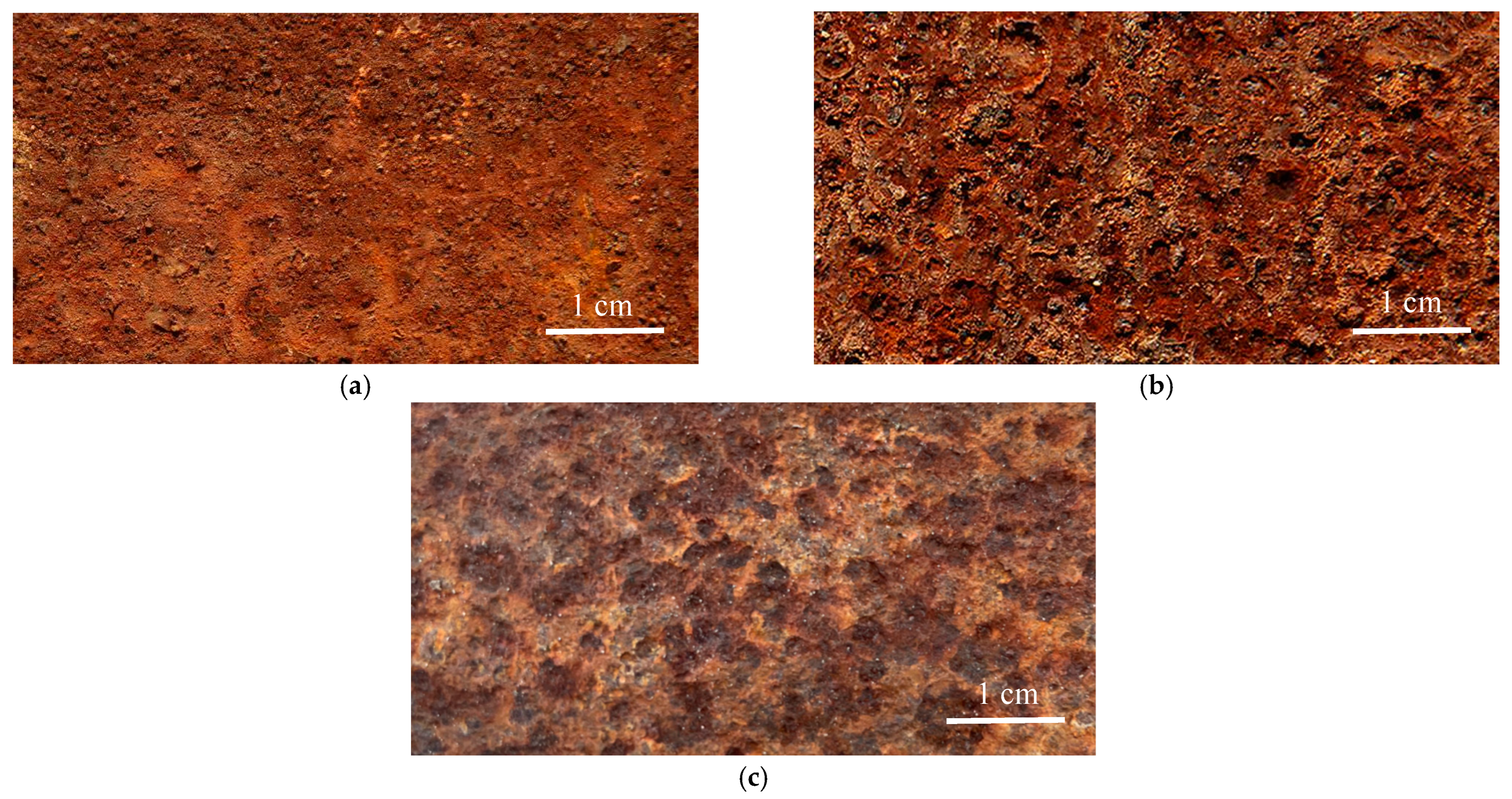
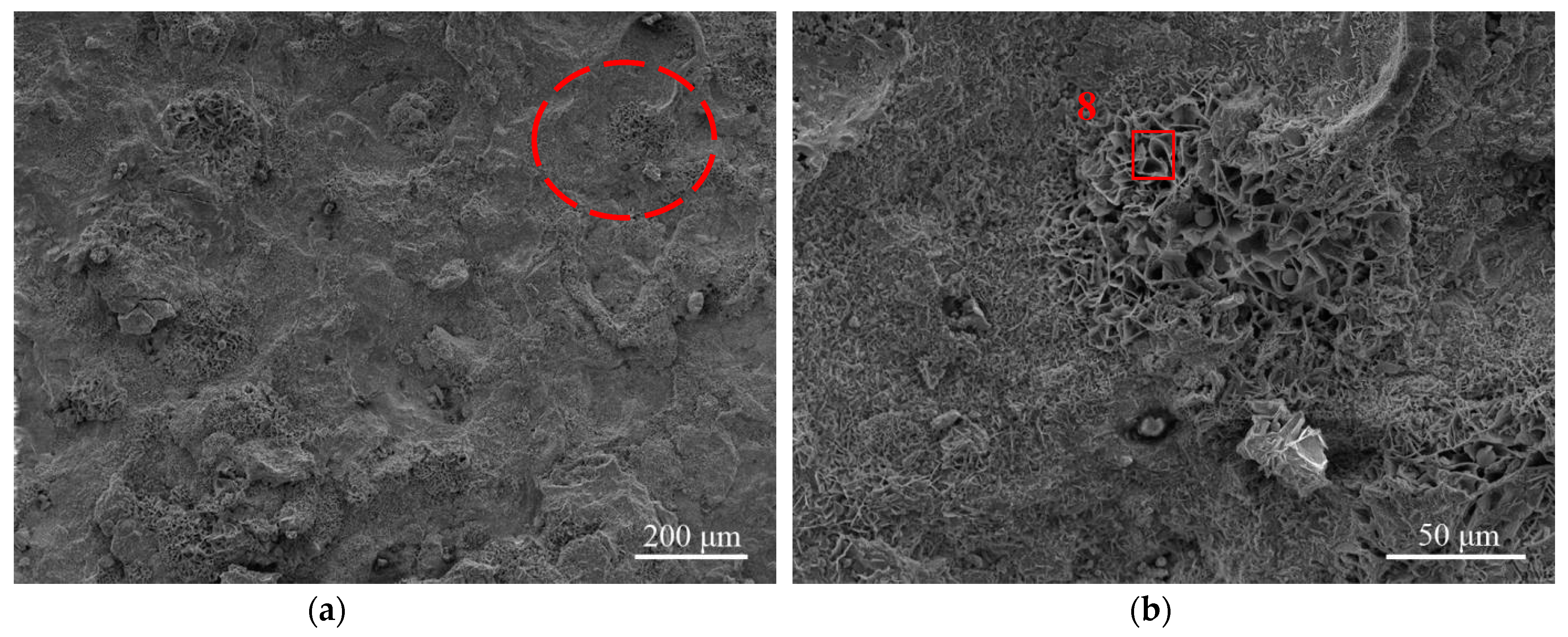
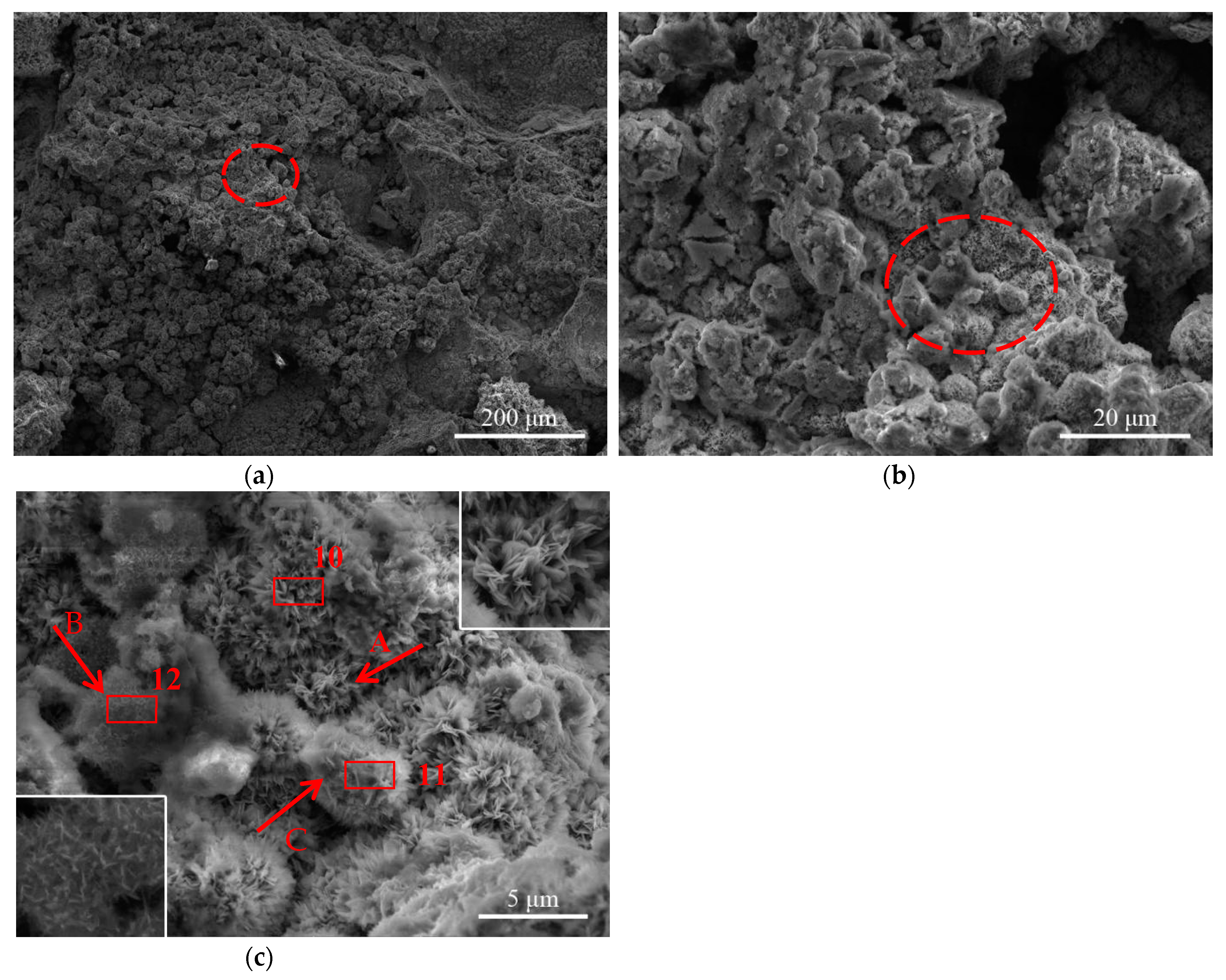
3.2. Morphologies of the Rust Layers

A digital camera was used to observe the macrosurface morphology of the rust layer exposed to an urban industrial atmosphere. As shown in Figure 3, after 12 months of atmospheric exposure, the rust layers were evenly distributed with red-brown colored loose structures. After 48 months of atmospheric exposure, the rust layers were red-brown with evenly distributed etch pits. After 84 months of atmospheric exposure, the rust layers were yellow-brown and dense, and the etch pits expanded. To summarize, as the corrosion time increased, the color of the rust layers deepened from red-brown to yellow-brown, revealing changes that occur gradually in the composition of the rust layers or the relative content of each component [61]. Furthermore, the rust layers thicken over time.

The SEM micro-morphology of the Q235B steel rust surface layer at 2, 12, 41, and 84 months of exposure to the urban industrial atmosphere is shown in Figure 4, Figure 5, Figure 6 and Figure 7. After 2 months of exposure, the corrosion products of the Q235 steel were relatively loose and flat, with areas of numerous bird’s nest formations (Figure 4a,b). After 12 months of corrosion, the corrosion products were mainly small particles, and the local corrosion products were loose and flat (Figure 5a,b). The loose and flat regions present mainly as worm’s nest formations (labeled “A” in Figure 5c,e). The particle regions (Figure 5c–f) were mainly hair-like formations (labeled “B”) in the bottom layer, cloud-like formations (labeled “C”) above, and the agglomeration (labeled “D”) of the two, globular formations with an amorphous appearance (labeled “E”), and globular formations with crystalline substructure in the form of needles (labeled “F”). After 41 months of corrosion, the corrosion products exhibited mainly particle shape with increased particle size and a tendency to compact into sheets (Figure 6a). The typical morphologies of corrosion products were laminar petal formations (labeled “A”), globular formations with a crystalline substructure (labeled “B”), and other globular formations composed of petal formations (labeled “C”) (Figure 6b,c). The hair-like and cloud-like structures shown in Figure 5f can still be observed after 41 months of corrosion. After 84 months of corrosion, some of the partial corrosion products were still loose, and some had compacted into dense, smooth corrosion layers with cracks (Figure 7a,b). The loose areas were dominated by granular corrosion products with different morphologies, including globular formations with crystalline substructures in the form of lamina (labeled “A”) and thin and flat sheet structures with whiskers (labeled “B”) (Figure 7c,e). The main corrosion products in the dense and smooth areas were cotton ball structures (labeled “C”) and compacted whisker structures (labeled “D”) (Figure 7d,f).

The corrosion products of Q235 structural steel exposed to the urban industrial atmospheric environment transformed from loose and flat to granular, and then to compact and smooth. Corrosion products of various forms interconnect and agglomerate loosely. They all have cavities and fractures, making the surface rust layers incapable of providing sufficient protection.

EDS analysis was performed on the surface of the rust layers, as presented in

Table 4. The element concentrations in corrosion products at different atmospheric exposure times (at. %).

Exposure Time (Month)	Location	O	Fe	C	Si	S	Mn	P	Al	K	In
2	Point 8 (Figure 4b)	44.1	37.8	17.5	0.4	0.2	——	——	——	——	——
12	Point 13 (Figure 5c)	41.1	42.8	15.2	0.2	0.5	0.1	——	——	——	——
	Point 14 (Figure 5c)	57.9	29.6	12.2	——	0.1	0.1	——	——	——	——
	Point 17 (Figure 5f)	51.3	35.3	12.8	0.1	0.2	0.2	0.1	——	——	——
	Point 19 (Figure 5f)	53.8	19.3	20.1	3.4	0.4	——	0.1	2.2	0.7	——
41	Point 10 (Figure 6c)	26.9	37.1	36	——	——	——	——	——	——	——
	Point 11 (Figure 6c)	8.4	91.6	——	——	——	——	——	——	——	——
	Point 12 (Figure 6c)	46.5	12.9	40.1	——	——	——	——	——	——	0.4
84	Point 41 (Figure 7e)	43	20.5	29.7	4.5	——	——	——	1.5	0.8	——
	Point 43 (Figure 7e)	51.6	16.7	30.3	1.4	——	——	——	——	——	——
	Point 45 (Figure 7d)	57.8	17.9	24.3	——	——	——	——	——	——	——

. The results show that the bird’s nest (Point 8 (Figure 4b)), worm’s nest (Point 14 (Figure 5c)), hair-like (Point 17 (Figure 5f)), and cloud-like morphological structures (Point 19 (Figure 5f)) and those formed from the agglomeration of cloud-like and hair-like structures (Point 13 (Figure 5c)) all contained sulfur. Sulfur was not detected in the laminar petal morphological or globular formations with crystalline substructures, or other globular formations composed of petal formations (Points 10–12 (Figure 6c)). Meanwhile, thin and flat sheet structures with whiskers and globular formations with crystalline substructures in the form of lamina (Points 41 and 43 (Figure 7e)) and compacted whisker structures also did not contain sulfur (Point 45 (Figure 7d)). Sulfur may come from the pollutants in the industrial atmosphere. The other elements that were detected, namely Si, Mn, Al, K, P, and In, were present on the surface of the rust layers, indicating that dust particles suspended in the atmosphere are deposited on the surface.

Figure 8 shows the cross-sectional morphologies of the rust layers at different urban industrial atmospheric exposure times. Distinguishable inner and outer rust layers were observed regardless of the exposure time. The inner layer was attached to the steel substrate with an irregular corrosion profile, i.e., the thickness of the inner rust layer was not uniform, which was mainly due to the non-uniform distribution of physical and chemical factors, such as environmental deposits and the direction of crystallites in the steel [3]. With the increase in corrosion time, the thickness of the inner rust layer increased; the thickness of the inner rust layer was about 0–50 mm after 12 months of atmospheric exposure (Figure 8a), 50–100 mm after 41 months (Figure 8b), and 100–200 mm after 84 months (Figure 8c). The dense inner rust layer, compactly attached to the steel, prevents the intrusion of corrosive media and protects the substrate from further corrosion. The thickness of the outer rust layer was uniform and tended to increase as the corrosion time increased. However, the overall thickness was thin because the stress caused by large temperature fluctuations and alternating wet/dry cycles [62] weakened the adhesion of the rust layers and caused them to detach easily. The outer rust layer was loose, had more cavities, cracks, and gaps, and was not tightly connected to the inner rust layer. Large cracks easily penetrate between the inner and outer rust layers, providing paths for corrosive media, mainly O₂ and SO₂. The outer layer had little inhibition against corrosive media and allowed further corrosion of the steel substrate to occur.

The EDS line surface scan image shown in Figure 8d corresponds to the yellow line in Figure 8b. Elemental analysis of the EDS spectrum shows a distinct boundary between the inner rust layer and the uncorroded steel substrate, where O and Fe content differences are most obvious. The corrosion products of the inner rust layer were mainly compounds that contained Fe and O. Corroded steels in urban industrial atmospheric environments have an obvious O and Fe content transition zone (about 5 μm in length) between the rust layer and steel substrate. The existence of the transition zone indicates that the corrosive media permeates and diffuses into the intact steel substrate adjacent to the rust layer through grain boundaries and adjacent areas, causing local corrosion (Figure 9).

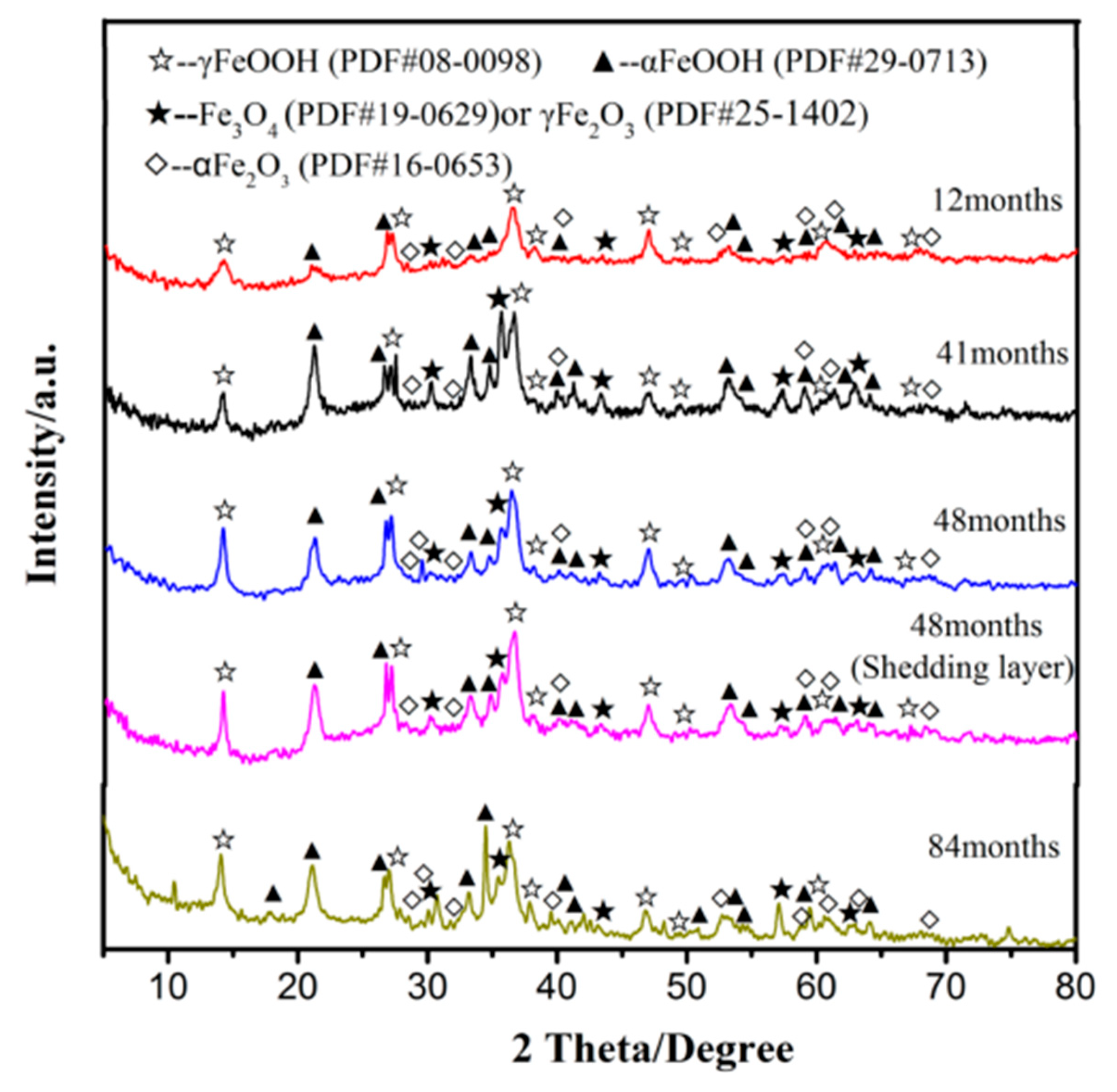
3.3. Phase Structures of the Rust Layers

Figure 10 shows the XRD spectrum of corrosion product powders scraped from the surface of the Q235B steel samples of different urban industrial atmospheric exposure times.

Table 5. Crystalline phases of corrosion products of Q235 steel formed at different times.

Time (Month)	α-FeOOH (Goethite) (%)	γ-FeOOH (Lepidocrocite) (%)	Fe3O4/γ-Fe2O3 (Magnetite/Maghemite) (%)	αFe2O3 (Hematite) (%)	α/γ
12	31.0	50.2	——	18.8	0.618
48	30.4	29.4	22.2	18.0	0.589
48 (Shedding layer)	30.9	21.4	34.3	13.4	0.554
84	39.2	24.5	35.6	0.7	0.652

shows a semi-quantitative analysis of the corrosion product content variation with time, which is expressed as a percentage of the total crystalline products found. Taking the atmospheric corrosion of the rust layer for 48 months as an example, the volume fractions of α-FeOOH, γ-FeOOH, and Fe₃O₄/γ-Fe₂O₃ phases obtained by the full spectrum fitting analysis using Highscore Plus software were 48.4%, 29.4%, and 22.2%, respectively, as illustrated in Figure 11. The partially similar phase structures of α-FeOOH and α-Fe₂O₃ cause overlapping XRD patterns that are indistinguishable. Hence, a peak splitting method was employed on the corresponding coincidence peak of the high index crystal plane, which was located near 2θ~59°, as plotted in Figure 12. Finally, the volume fractions of α-FeOOH and α-Fe₂O₃ were determined to be 30.4% and 18.0%, respectively, according to the area ratio. Similarly, the content of corrosion products at other corrosion times could be obtained using the aforementioned method, as presented in Table 5.

Based on Figure 10 and Table 5, it can be concluded that the main crystalline phases of the rust layers were α-FeOOH, γ-FeOOH, and Fe₃O₄/γ-Fe₂O₃. The corrosion products after one year of atmospheric corrosion contained mainly γ-FeOOH, followed by α-FeOOH. Fe₃O₄/γ-Fe₂O₃ did not reach the content level required for semi-quantitative analysis. After 41 months of corrosion, the γ-FeOOH peak did not change significantly, while the α-FeOOH and Fe₃O₄/γ-Fe₂O₃ peaks narrowed in width and increased in intensity. After 48 months of corrosion, the composition of the shedding rust layer was approximately the same as that still attached to the steel. The content of Fe₃O₄/γ-Fe₂O₃ in the rust layer increased, while γ-FeOOH decreased. After 84 months of corrosion, the content of α-FeOOH increased, and Fe₃O₄/γ-Fe₂O₃ continued to increase.

The XRD results in Figure 10 indicate the presence of α-Fe₂O₃ in the urban industrial atmosphere, which is consistent with the detection of α-Fe2O3 in the industrial atmosphere in the literature [4,10,63]. After 84 months of corrosion, the α-Fe₂O₃ content decreased significantly.

4. Discussions

4.1. Prediction of Corrosion Rates

The mass loss of Q235 steel after long-term exposure to the urban industrial atmosphere demonstrated that the steel undergoes a continuous process of corrosion (Figure 2). In the first two years of exposure corrosion, the rust layers were thin (Figure 8a) and loose (Figure 3a, Figure 4, Figure 5 and Figure 8a). During this period, it was not easy to accumulate pollutants under rainfall erosion, and liquid films evaporated easily under long sunshine hours (Table 3). Therefore, corrosion was relatively difficult to occur. From the third year to about the first half of the fourth year, the rust layer grew to a certain thickness (Figure 8b) but remained loose (Figure 3b and Figure 6), and the SO₂ concentration was high. Many pores (voids) and microcracks in the rust layer (Figure 8b) provided access to the corrosive media, making the rust layers highly permeable, whereas the rust layer shielded the sunlight and impeded the rust layers from drying. Consequently, the corrosion rate increased, and this agrees well with the other available results [25]. When the corrosion time is less than 3 years, the n value is 1.317, and this is consistent with the other available result [64], that is, corrosion is more serious in industrial regions than on the coast. However, the corrosion rate during the fourth year showed a decrease compared to the third year. After four years of corrosion, the corrosion rate decreased significantly, which resembles the rule of corrosion in an industrial atmosphere described in one study [4]. After seven years of corrosion, the n value for the second stage of corrosion was found to be 0.614, indicating that corrosion after four years is a decelerated and convergent process. The deceleration in corrosion rate can be explained by recrystallization, agglomeration, and compaction of rust layers as time increases, making the rust layers denser (Figure 3c). Parts of the rust layers became dense and smooth (Figure 7b,d). The dense rust layer impedes the diffusion of reactants, thus slowing down the corrosion rate [65,66,67,68]. Furthermore, as shown in Table 3, the air quality of Taiyuan significantly improved in the preceding years, and the concentration of SO₂ in 2018 decreased by 63.73% compared with that in 2013. Therefore, corrosion caused by SO₂ decreased significantly after the fifth year.

Based on the results mentioned above, it can be concluded that the corrosion power function parameters of Q235 steel, obtained after three years of exposure to corrosive environments, do not entirely reflect the corrosion performance in highly corrosive environments. This conclusion is consistent with the conclusions of some previous studies [25,69]. Reliable atmospheric corrosion parameters can only be derived from long-term exposure. It is inappropriate to apply the results of one year of atmospheric corrosion to determine the corrosivity of the environment.

4.2. Evolution of Corrosion Products

In an urban industrial atmosphere, complex electrochemical reactions occur on steel surfaces. The phase composition of the rust layers depends mainly on the anions in the electrolyte film. The content of dissolved oxygen at the metal/rust layer interface is relatively high, and the cathode is mainly oxygen reduction, an oxygen-absorbing corrosion (Equations (2) and (3)). The initially generated Fe (OH)₂ is unstable. Some of the Fe(OH)₂ rapidly oxidizes to Fe(OH)₃ (Equation (4)), which is partially dehydrated to generate red-brown Fe₂O₃.nH₂O. Some of the Fe (OH)₂ may generate FeOOH in the presence of O₂ (Equation (5)) [70,71].

$$\mathrm{A}\mathrm{n}\mathrm{o}\mathrm{d}\mathrm{e}:\mathrm{F}\mathrm{e}\to \mathrm{F}{\mathrm{e}}^{2+}+2{\mathrm{e}}^{-}$$

(2)

$$\mathrm{C}\mathrm{a}\mathrm{t}\mathrm{h}\mathrm{o}\mathrm{d}\mathrm{e}:{\mathrm{O}}_2+4\mathrm{e}+2{\mathrm{H}}_2\mathrm{O}\to 4\mathrm{O}{\mathrm{H}}^{-}$$

(3)

The main pollutant in Taiyuan is SO₂, which is easily soluble in water. The thin liquid film on the steel surface absorbs SO₂ from the atmosphere to generate H₂SO₃. A small amount of H₂SO₃ is gradually oxidized to H₂SO₄, which reduces the electrolyte pH, accelerates the dissolution of the anode, and speeds up the corrosion rate of the steel (Equations (6) and (7)) [37,72].

$$2\mathrm{F}\mathrm{e}{\left(\mathrm{O}\mathrm{H}\right)}_2+1/2{\mathrm{O}}_2+{\mathrm{H}}_2\mathrm{O}\to 2\mathrm{F}\mathrm{e}{\left(\mathrm{O}\mathrm{H}\right)}_3$$

(4)

$$2\mathrm{F}\mathrm{e}{\left(\mathrm{O}\mathrm{H}\right)}^{+}+1/2{\mathrm{O}}_2+2\mathrm{O}{\mathrm{H}}^{-}\to 2\mathrm{F}\mathrm{e}\mathrm{O}\mathrm{O}\mathrm{H}+{\mathrm{H}}_2\mathrm{O}$$

(5)

$$4\mathrm{F}\mathrm{e}\mathrm{S}{\mathrm{O}}_4+6{\mathrm{H}}_2\mathrm{O}+{\mathrm{O}}_2\to 4\mathrm{F}\mathrm{e}\mathrm{O}\mathrm{O}\mathrm{H}+4{\mathrm{H}}_2\mathrm{S}{\mathrm{O}}_4$$

(6)

$$2{\mathrm{H}}_2\mathrm{S}{\mathrm{O}}_4+2\mathrm{F}\mathrm{e}+{\mathrm{O}}_2\to 2\mathrm{F}\mathrm{e}\mathrm{S}{\mathrm{O}}_4+2{\mathrm{H}}_2\mathrm{O}$$

(7)

After two months of exposure to the atmospheric environment, numerous areas with bird’s nest structures formed in the corrosion products of Q235 steel (Figure 4). The bird’s nest structure is a typical morphology of γ-FeOOH [4,12,31,73,74]. Therefore, the main corrosion products after two months of exposure are γ-FeOOH.

After 12 months of corrosion, the worm’s nest structure (labeled “A” in Figure 5c,e), the hair-like structure (labeled “B” in Figure 5f), and the globular structure with an amorphous appearance (labeled “E” in Figure 5c,d), are all the morphologies of γ-FeOOH [73,74]; the cloud-like structures (labeled “C” in Figure 5f) were probably morphologies of α-FeOOH [31]; the globular structure formed by the agglomeration of cloud-like and hair-like structures (labeled “D” in Figure 5f), and the globular formation with a crystalline substructure in the form of a needle(labeled “F” in Figure 5e), are all mixtures of γ-FeOOH and α-FeOOH [73,74].

Figure 6c shows the typical morphologies of γ-FeOOH and α-FeOOH formed on steel after 41 months of corrosion. α-FeOOH appears as laminar petal formations (labeled “A”) [73], and γ-FeOOH is globular with crystalline substructures (labeled “B”) [73,74]. Some petal structures also appear in the globular formations (labeled “C”) and are a mixture of γ-FeOOH and α-FeOOH.

These features may indicate growing α-FeOOH that was replacing lepidocrocite. The main corrosion product in the initial stages of corrosion is γ-FeOOH, but with increasing exposure time, γ-FeOOH is converted into amorphous FeOOH through dissolution and precipitation, and then gradually transforms into α-FeOOH [75] (Equation (8)). Yamashita et al. [45] also believed that the amorphous inner layer of steel may transform into densely packed goethite nanoparticles during long-term exposure. The XRD results in Figure 10 and Table 5 further support that within one year of atmospheric corrosion, the corrosion products were mainly γ-FeOOH, followed by α-FeOOH. SO₂ is generally considered to be the most corrosive gas in the atmosphere [76] and contributes to the formation of α-FeOOH [77,78].

$$\mathsf{\gamma }-\mathrm{F}\mathrm{e}\mathrm{O}\mathrm{O}\mathrm{H}\to \mathrm{F}\mathrm{e}{\mathrm{O}}_x{\left(\mathrm{O}\mathrm{H}\right)}_{3-2x}\to \mathsf{\alpha }-\mathrm{F}\mathrm{e}\mathrm{O}\mathrm{O}\mathrm{H}$$

(8)

As the corrosion reached 48 months, the content of α-FeOOH exceeded that of γ-FeOOH, and the Fe₃O₄/γ-Fe₂O₃ content increased to 22.2–34.3% (Table 5). The formation of Fe₃O₄ content indicated that the reduction reaction from Fe³⁺ to Fe²⁺ occurs in the rust layer [64,79,80,81], and the rust layer on the steel surface acts as a strong oxidant during the wetting process. That is, some of the γ-FeOOH becomes a cathode depolarizing agent and is reduced to black Fe₃O₄ (Equation (9)) [73,82], while some is dissolved to form γ-Fe₂O₃. The Fe₃O₄ content after 48 months of exposure was higher than that after 12 months (Figure 10; Table 5). This is due to the fact that the rust layer becomes thicker after 48 months of exposure, which makes it difficult for the inside of the rust layer to dry out. The longer the rust layer remains in the infiltration state, the more conducive it is to the formation of Fe₃O₄. In addition, Fe₃O₄ is typically formed near the steel substrate [83,84], where the lower oxygen availability favors its development (Equation (10)) [85,86]. The continuously generated α-FeOOH increased the stability of the rust layer and strengthened its protectivity. This decreases the corrosion rate. However, magnetite that usually forms close to the steel substrate has high conductivity and acts as a large cathode area, which, from an electrochemical perspective, accelerates subsequent corrosion stages (as described by Equation (10)). Therefore, higher levels of magnetite are associated with lower protection by the formed rust layer, and increased magnetite content is conducive to an increased corrosion rate in long-term atmospheric corrosion [87].

$$8\mathsf{\gamma }-\mathrm{F}\mathrm{e}\mathrm{O}\mathrm{O}\mathrm{H}+\mathrm{F}{\mathrm{e}}^{2+}+2{\mathrm{e}}^{-}\to 3\mathrm{F}{\mathrm{e}}_3{\mathrm{O}}_4+4{\mathrm{H}}_2\mathrm{O}$$

(9)

$$4\mathrm{F}{\mathrm{e}}_3{\mathrm{O}}_4+{\mathrm{O}}_2+6{\mathrm{H}}_2\mathrm{O}\to 12\mathsf{\gamma }-\mathrm{F}\mathrm{e}\mathrm{O}\mathrm{O}\mathrm{H}$$

(10)

According to studies, Fe₃O₄/γ-Fe₂O₃ formed by long-term exposure to the atmosphere usually exists in the inner rust layer [30,88], implying that it is difficult to observe the micromorphology of Fe₃O₄/γ-Fe₂O₃ in the SEM on the outermost surface of the rust layer.

After 84 months of corrosion, the content of α-FeOOH continued to increase, eventually reaching 39.2%, and the Fe₃O₄/γ-Fe₂O₃ content increased, reaching 35.6% (Figure 10; Table 5). The globular formations with crystalline substructures in the form of lamina (labeled “A” in Figure 7e) are γ-FeOOH [73,74]; the thin and flat structures with whiskers (labeled “B” in Figure 7e) and cotton ball structures (labeled “C” in Figure 7f) are α-FeOOH [4,31]. From the surface morphologies and the rust layer cross-sections (Figure 3c, Figure 7 and Figure 8), we can see that the thickness of the rust layer continuously increased (Figure 8c) and became denser after 84 months of long-term corrosion, while it is very easy to find very open structures such as large porosity (Figure 7c), spallation (Figure 13a), and cracking (Figure 7d and Figure 13b) in the rust layer, providing access for corrosive media. Irregular cracks (Figure 7d and Figure 13b) are typical manifestations of highly aggressive atmospheric corrosion [4]. The more corrosive the atmosphere is, the easier it is to find open structures [4].

The water-soluble FeSO₄ is expected to be present, and although the EDS results detected sulfur in the morphometric regions (Figure 4 and Figure 5, Table 4), FeSO₄ was not detected by the EDS (Figure 10, Table 5). This may be due to its insufficiency for detection by the instrument. Presumably, the anions (SO₄²⁻) migrate into the etch pits, thus hiding themselves underground [89], so the content of FeSO₄ in the rust layer samples is very low.

The XRD results indicate that α-Fe₂O₃ is present in the industrial atmosphere, and the acid rain is conducive to its transformation (Figure 10, Table 5) [4]. After 84 months of corrosion, the content of α-Fe₂O₃ decreased significantly. This is mainly because the concentration of SO₂ in the atmosphere decreased significantly (Table 3).

The corrosion rate of steel in any environment depends on the composition of the rust layer, especially the α/γ ratio, where α is the volume fraction of α-FeOOH or the sum of the volume fractions of α-FeOOH and amorphous rust, and γ is the sum of the volume fractions of γ-FeOOH, β- FeOOH, and Fe₃O₄ [45,90]. The value of α in Table 4 represents the volume fraction of α-FeOOH, and γ is the sum of the volume fractions of γ-FeOOH and Fe₃O₄. XRD could not distinguish between maghemite (γ-Fe₂O₃) and magnetite (Fe₃O₄), so the contributions of both were attributed to magnetite (Fe₃O₄). It can be seen from Table 5 that when the exposure time was no more than 48 months, the α/γ ratio decreased with increasing exposure time, indicating weak protection by the rust layer and a high corrosion rate. After 84 months of corrosion, the α/γ ratio increased to 0.652, indicating that the protection of the rust layer increased and the corrosion rate slowed down, which is consistent with the previous discussion.

In summary, the corrosion mechanism of Q235 steel in urban industrial atmospheric environments is illustrated in Figure 14. In the first four years of atmospheric corrosion, the SO₂ concentration was high (Table 3), and the corrosion mechanism was mainly governed by the acid cycle reaction mechanism shown on the left side. This action will continue with an electrochemically conducting limb (FeSO₄ in a wet state) and an electronically conducting limb (Fe₃O₄), and the corrosion rate of Q235 steel was fast (Figure 2). In the fifth year of atmospheric corrosion, there was a decrease in the SO₂ concentration (Table 3), and the electrochemical reaction was gradually dominated by oxygen-absorbing corrosion (shown on the right side), resulting in a decrease in the corrosion rate of Q235 steel over time (Figure 2).

5. Conclusions

This study investigated the corrosion behavior and mechanisms of Q235 steel exposed to the typical industrial atmosphere (Taiyuan) for seven years. The conclusions are obtained as follows:

(1)

The corrosion kinetics of Q235 steel exposed to the urban industrial atmosphere for a long term follow a two-stage corrosion power function law. The atmospheric corrosion evolution law for short-term exposure differs from that for long-term exposure. Therefore, the short-term corrosion test results fail to fully reflect the corrosion performance of Q235 steel in these environments. SO₂ significantly affects the corrosion behavior of steel.

(2)

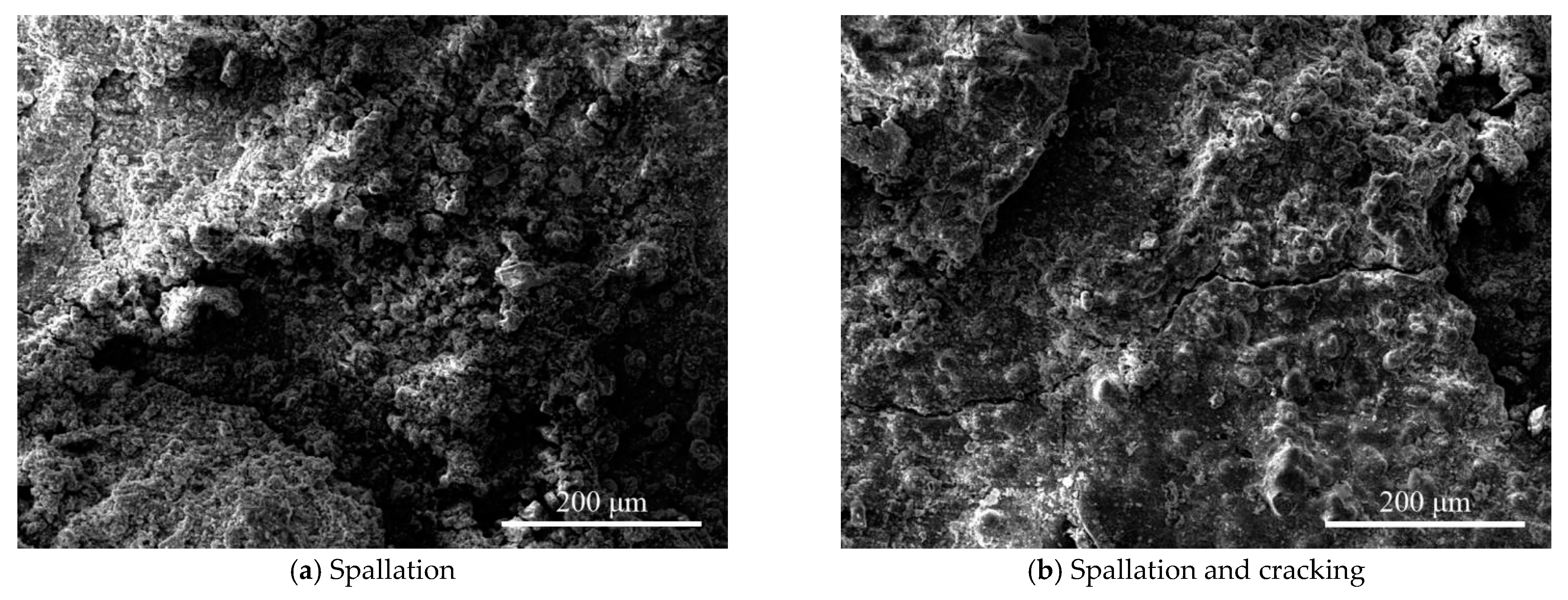
The morphology of the corrosion products of Q235 steel in the urban industrial atmosphere changes from loose and flat to granular, and finally to compact and smooth. Although the outer rust layer was easy to fall off, the thickness of the inner and outer rust layers increases with increased exposure time. The various forms of corrosion products connect and agglomerate with each other and possess cavities, cracks, and spallation, reducing the rust layer’s protection.

(3)

The rust layer crystalline phase contains α-FeOOH, γ-FeOOH, Fe₃O₄/γ-Fe₂O₃, and α-Fe₂O₃ in the urban industrial atmosphere. Corrosion products in the initial period are mainly γ-FeOOH, followed by α-FeOOH, and only a small amount of Fe₃O₄/γ-Fe₂O₃. With the increase in exposure time, α-FeOOH and Fe₃O₄/γ-Fe₂O₃ in the rust layer increases. The concentration of SO₂ in the atmosphere affects the formation of α-Fe₂O₃. In long-term atmospheric corrosion, the increase in Fe₃O₄/γ-Fe₂O₃ content is beneficial to improving the corrosion rate.

(4)

In the urban industrial atmosphere, γ-FeOOH typically has bird’s nest structures, worm’s nest structures, globular structures with crystalline substructures, and hair-like structures; α-FeOOH has laminar petal structures, cloud-like structures, laminar structures with whiskers, and cotton ball structures.

(5)

The corrosion rate is impacted by the composition of the rust layer and can be measured with the α/γ ratio. When the exposure time is no more than 48 months, α/γ decreases with the increasing exposure time, indicating weak rust layer protection and a high corrosion rate. After 84 months of corrosion, α/γ increases, indicating increased rust layer protection and a decreased corrosion rate.

References

1. Quintana, P.; Veleva, L.; Cauich, W.; Pomes, R.; Peña, J.L. Study of the composition and morphology of initial stage of corrosion products formed on Zn plates exposed to the atmosphere of southeast Mexico. Appl. Surf. Sci. 1996, 99, 325–334. [Google Scholar] [CrossRef]
2. Ma, Y.; Li, Y.; Wang, F. Corrosion of low carbon steel in atmospheric environments of different chloride content. Corros. Sci. 2009, 51, 997–1006. [Google Scholar] [CrossRef]
3. Asami, K.; Kikuchi, M. In-depth distribution of rusts on a plain carbon steel and weathering steels exposed to coastal–industrial atmosphere for 17 Years. Corros. Sci. 2003, 45, 2671–2688. [Google Scholar] [CrossRef]
4. de la Fuente, D.; Diaz, I.; Simancas, J.; Chico, B.; Morcillo, M. Long-term atmospheric corrosion of mild steel. Corros. Sci. 2011, 53, 604–617. [Google Scholar] [CrossRef] [Green Version]
5. Hou, B.Y. Corrosion Control Technology of Marine Steel Structure in Splash Zone; Science Press: Beijing, China, 2011; pp. 1–2. (In Chinese) [Google Scholar]
6. Bhaskaran, R.; Palaniswamy, N.S.; Rengaswamy, N.; Jayachandran, M. ASM Hand Book. ASM Int. Met. Park Ohio 2005, 13B, 619. [Google Scholar]
7. Schmitt, G.; Schütze, M.; Hays, G.F.; Burns, W.; Jacobson, G. Global Needs for Knowledge Dissemination, Research, and Development in Materials Deterioration and Corrosion Control; World Corrosion Organization: New York, NY, USA, 2009. [Google Scholar]
8. Arroyave, C.; Lopez, F.A.; Morcillo, M. The early atmospheric corrosion stages of carbon steel in acidic fogs. Corros. Sci. 1995, 37, 1751–1761. [Google Scholar] [CrossRef] [Green Version]
9. Han, W.; Yu, G.C.; Wang, Z.Y.; Wang, J. Characterisation of initial atmospheric corrosion carbon steels by field exposure and laboratory simulation. Corros. Sci. 2007, 49, 2920–2935. [Google Scholar] [CrossRef]
10. Han, W.; Pan, C.; Wang, Z.Y.; Yu, G.C. A study on the initial corrosion behavior of carbon steel exposed to outdoor wet-dry cyclic condition. Corros. Sci. 2014, 88, 89–100. [Google Scholar] [CrossRef]
11. Yan, S.T.; Jin, Y.; Xu, F.F.; Wen, L. Influence of deposited atmospheric particulates on initial corrosion behavior of mild steel. Corros. Sci. Prot. Technol. 2019, 31, 467–474. (In Chinese) [Google Scholar]
12. Song, X.X.; Huang, S.P.; Wang, C.; Wang, Z.Y. The Initial corrosion behavior of carbon steel exposed to the coastal-Industrial atmosphere in Hongyanhe. Acta Metall. Sin. 2020, 56, 1355–1365. (In Chinese) [Google Scholar]
13. Rodríguez, J.J.S.; Hernandez, F.J.S.; Gonzalez, J.E.G. The effect of environmental and meteorological variables on atmospheric corrosion of carbon steel, copper, zinc and aluminium in a limited geographic zone with different types of environment. Corros. Sci. 2003, 45, 799–815. [Google Scholar] [CrossRef]
14. Lan, T.T.N.; Thoa, N.T.P.; Nishimura, R.; Tsujino, Y.; Yokoi, M.; Maeda, Y. Atmospheric corrosion of carbon steel under field exposure in the southern part of Vietnam. Corros. Sci. 2006, 48, 179–192. [Google Scholar] [CrossRef]
15. Corvo, F.; Betancourt, N.; Mendoza, A. The Influence of airborne salinity on the atmospheric corrosion of steel. Corros. Sci. 1995, 37, 1889–1901. [Google Scholar] [CrossRef]
16. Castaño, J.G.; Botero, C.A.; Restrepo, A.H.; Agudelo, E.A.; Correa, E.; Echeverría, F. Atmospheric corrosion of carbon steel in Colombia. Corros. Sci. 2010, 52, 216–223. [Google Scholar] [CrossRef]
17. Corvo, F.; Mendoza, A.R.; Autie, M.; Betancourt, N. Role of water adsorption and salt content in atmospheric corrosion products of steel. Corros. Sci. 1997, 39, 815–820. [Google Scholar] [CrossRef]
18. Song, Z.B.; Wang, Z.C.; Wang, J.G.; Peng, B.; Zhang, C.Z. Atmospheric corrosion behavior of Q235 Steel in northern Hebei region. Mater. Mech. Eng. 2021, 45, 46–51. (In Chinese) [Google Scholar]
19. Cole, I.S.; Ganther, W.D.; Sinclair, J.D.; Lau, D.; Paterson, D.A. A study of the wetting of metal surfaces in order to understand the processes controlling atmospheric corrosion. J. Electrochem. Soc. 2004, 151, B627–B635. [Google Scholar] [CrossRef]
20. Mansfeld, F.; Kenkel, J.V. Electrochemical measurement of time-of-wetness and atmospheric corrosion rates. Corrosion 1977, 33, 13–16. [Google Scholar] [CrossRef]
21. Dean, S.; Reiser, D.B. Analysis of long-term atmospheric corrosion results from ISOCORRAG Program. In Outdoor Atmospheric Corrosion, ASTM STP 1421; Towsend, H.E., Ed.; American Society for Testing and Materials: Philadelphia, PA, USA, 2002; pp. 3–18. [Google Scholar]
22. Ma, Y.T.; Li, Y.; Wang, F.H. The atmospheric corrosion kinetics of low carbon steel in a tropical marine environment. Corros. Sci. 2010, 52, 1796–1800. [Google Scholar] [CrossRef]
23. Melchers, R.E.; Jeffrey, R. The critical involvement of anaerobic bacterial activity in modelling the corrosion behaviour of mild steel in marine environments. Electrochim. Acta 2008, 54, 80–85. [Google Scholar] [CrossRef]
24. Melchers, R.E. Long-term corrosion of cast irons and steel in marine and atmospheric environments. Corros. Sci. 2013, 68, 186–194. [Google Scholar] [CrossRef]
25. Liang, C.F.; Hou, W.T. Sixteen-year atmospheric corrosion exposure study of steel. J. Chin. Soc. Corros. Prot. 2005, 25, 1–6. (In Chinese) [Google Scholar]
26. Liang, C.F.; Hou, W.T. Eight-year atmospheric corrosion exposure study of steel. Corros. Sci. Prot. Technol. 1995, 7, 183–186. (In Chinese) [Google Scholar]
27. Mao, H.R.; Qu, G.C.; Huang, S.Y.; Zhang, Q.Y. Atmospheric corrosion of carbon steels and low alloy steel exposed in Guangzhou. Environ. Technol. 2001, 3, 5–7. (In Chinese) [Google Scholar]
28. Zhi, Y.J.; Yang, T.; Fu, D.M. An improved deep forest model for forecast the outdoor atmospheric corrosion rate of low-alloy steels. J. Mater. Sci. Technol. 2020, 49, 202–210. [Google Scholar] [CrossRef]
29. Song, X.X.; Wang, K.Y.; Zhou, L.J.; Chen, Y.J.; Ren, K.X.; Wang, J.Y.; Zhang, C. Multi-factor mining and corrosion rate prediction model construction of carbon steel under dynamic atmospheric corrosion environment. Eng. Fail. Anal. 2022, 134, 105987. [Google Scholar] [CrossRef]
30. Oh, S.J.; Cook, D.; Townsend, H. Atmospheric corrosion of different steels in marine, rural and industrial environments. Corros. Sci. 1999, 41, 1687–1702. [Google Scholar] [CrossRef]
31. Fonna, S.; Ibrahim, I.B.M.; Gunawarman; Huzni, S.; Ikhsan, M.; Thalib, S. Investigation of corrosion products formed on the surface of carbon steel exposed in Banda Aceh’s atmosphere. Heliyon 2021, 7, e06608. [Google Scholar] [CrossRef] [PubMed]
32. Antunes, R.A.; Costa, I.; de Faria, D.L.A. Characterization of corrosion products formed on steels in the first months of atmospheric exposure. Mater. Res. 2003, 6, 403–408. [Google Scholar] [CrossRef] [Green Version]
33. Oh, S.J.; Cook, D.C.; Carpio, J.J. Characterization of the corrosion products formed on carbon steel in a marine environment. J. Korean Phys. Soc. 2000, 36, 106–110. [Google Scholar]
34. Wang, Z.G.; Hai, C.; Jiang, J.; Lan, X.S.; Du, C.W.; Li, X.G. Corrosion behavior of Q235 steels in atmosphere at Deyang District for one Year. J. Chin. Soc. Corros. Prot. 2021, 41, 871–876. (In Chinese) [Google Scholar]
35. Tian, Q.Q.; Hai, C.; Wang, Z.G.; Wang, N.H.; Lan, X.S.; Du, C.W. Study on corrosion behavior of Q235 carbon steel in typical atmospheric pollution environment in Leshan, Sichuan province. J. Southwest Minzu Univ. 2020, 46, 478–486. (In Chinese) [Google Scholar]
36. Wang, C.; Cao, G.W.; Pan, C.; Wang, Z.Y.; Liu, M.R. Atmospheric corrosion of carbon steel and weathering steel in three environments. J. Chin. Soc. Corros. Prot. 2016, 36, 39–46. (In Chinese) [Google Scholar]
37. Mi, F.Y.; Wang, X.D.; Liu, Z.P.; Wang, B.; Peng, Y.; Tao, D.P. Industrial atmospheric corrosion resistance of P-RE weathering steel. J. Iron Steel Res. Int. 2011, 18, 67–73. [Google Scholar] [CrossRef]
38. Díaz, I.; Cano, H.; Lopesino, P.; de la Fuente, D.; Chico, B.; Jiménez, J.A.; Medina, S.F.; Morcillo, M. Five-year atmospheric corrosion of Cu, Cr and Ni weathering steels in a wide range of environments. Corros. Sci. 2018, 141, 146–157. [Google Scholar] [CrossRef]
39. Cheng, X.; Jin, Z.; Liu, M.; Li, X. Optimizing the nickel content in weathering steels to enhance their corrosion resistance in acidic atmospheres. Corros. Sci. 2017, 115, 135–142. [Google Scholar] [CrossRef]
40. Yu, Q.; Dong, C.F.; Fang, Y.H.; Xiao, K.; Guo, C.Y.; He, G.; Li, X.G. Atmospheric corrosion of Q235 carbon steel and Q450 weathering steel in Turpan, China. J. Iron Steel Res. Int. 2016, 23, 1061–1070. [Google Scholar] [CrossRef]
41. Dong, B.J.; Liu, W.; Zhang, T.Y.; Chen, L.J.; Fan, Y.M.; Zhao, Y.G.; Yang, W.J.; Banthukul, W. Corrosion failure analysis of low alloy steel and carbon steel rebar in tropical marine atmospheric environment: Outdoor exposure and indoor test. Eng. Fail. Anal. 2021, 129, 105720. [Google Scholar] [CrossRef]
42. Wu, W.; Cheng, X.; Hou, H.; Liu, B.; Li, X. Insight into the product film formed on Ni-advanced weathering steel in a tropical marine atmosphere. Appl. Surf. Sci. 2018, 436, 80–89. [Google Scholar] [CrossRef]
43. Jia, J.; Wu, W.; Cheng, X.; Zhao, J. Ni-advanced weathering steels in Maldives for two years: Corrosion results of tropical marine field test. Constr. Build. Mater. 2020, 245, 118463. [Google Scholar] [CrossRef]
44. Vassie, P.R.; Mckenzie, M. Electrode potentials for on-site monitoring of atmospheric corrosion of steel. Corros. Sci. 1985, 25, 1–13. [Google Scholar] [CrossRef]
45. Yamashita, M.; Miyuki, H.; Matsuda, Y.; Nagano, H.; Misawa, T. The long term growth of the protective rust layer formed on weathering steel by atmospheric corrosion during a quarter of a century. Corros. Sci. 1994, 36, 283–299. [Google Scholar] [CrossRef]
46. Kamimura, T.; Hara, S.; Miyuki, H.; Yamashita, M.; Uchida, H. Composition and protective ability of rust layer formed on weathering steel exposed to various environments. Corros. Sci. 2006, 48, 2799–2812. [Google Scholar] [CrossRef]
47. Nishimura, T. Rust formation and corrosion performance of Si- and Al-bearing ultrafine grained weathering steel. Corros. Sci. 2008, 50, 1306–1312. [Google Scholar] [CrossRef]
48. Tamura, H. The role of rusts in corrosion and corrosion protection of iron and steel. Corros. Sci. 2008, 50, 1872–1883. [Google Scholar] [CrossRef] [Green Version]
49. Murayama, M.; Nishimura, T.; Tsuzaki, K. Nano-scale chemical analysis of rust on a 2% Si-bearing low alloy steel exposed in a coastal environment. Corros. Sci. 2008, 50, 2159–2165. [Google Scholar] [CrossRef]
50. Samie, F.; Tidblad, J.; Kucera, V.; Leygraf, C. Atmospheric corrosion effects of HNO3—Comparison of laboratory-exposed copper, zinc and carbon steel. Atmos. Environ. 2007, 41, 4888–4896. [Google Scholar] [CrossRef]
51. Morcillo, M.; Chico, B.; Díaz, I.; Cano, H.; de la Fuente, D. Atmospheric corrosion data of weathering steels. A Review. Corros. Sci. 2013, 77, 6–24. [Google Scholar] [CrossRef] [Green Version]
52. Mendoza, A.R.; Corvo, F. Outdoor and indoor atmospheric corrosion of carbon steel. Corros. Sci. 1999, 41, 75–86. [Google Scholar] [CrossRef]
53. Corvo, F.; Torrens, A.D.; Betancourt, N.; Pérez, J.; Gonzalez, E. Indoor atmospheric corrosion in Cuba. A report about indoor localized corrosion. Corros. Sci. 2007, 49, 418–435. [Google Scholar] [CrossRef]
54. Tidblad, J. Atmospheric corrosion of metals in 2010–2039 and 2070–2099. Atmos. Environ. 2012, 55, 1–6. [Google Scholar] [CrossRef]
55. Wang, L.; Guo, C.Y.; Xiao, K.; Silayiding, T.; Dong, C.F.; Li, X.G. Corrosion behavior of carbon steels Q235 and Q450 in dry hot atmosphere at Turpan District for four years. J. Chin. Soc. Corros. Prot. 2018, 38, 431–437. (In Chinese) [Google Scholar]
56. Wu, H.Y.; Lei, H.G.; Chen, Y.F.; Qiao, J.Y. Comparison on corrosion behaviour and mechanical properties of structural steel exposed between urban industrial atmosphere and laboratory simulated environment. Constr. Build. Mater. 2019, 211, 228–243. [Google Scholar] [CrossRef]
57. Wu, H.Y.; Lei, H.G.; Chen, Y.F. Study on corrosion models of structural steel exposed in urban industrial atmospheric and laboratory simulated environments based on the 3D profile. Thin-Walled Struct. 2021, 168, 108286. [Google Scholar] [CrossRef]
58. Wu, H.Y.; Lei, H.G.; Chen, Y.G. Grey relational analysis of static tensile properties of structural steel subjected to urban industrial atmospheric corrosion and accelerated corrosion. Constr. Build. Mater. 2022, 315, 125706. [Google Scholar] [CrossRef]
59. Wu, H.Y.; Lei, H.G.; Chen, Y.F. Comparison on mechanisms of high-cycle fatigue performance of structural steel exposed to urban industrial atmosphere and laboratory simulated corrosive environment based on infrared thermography. Int. J. Fatigue 2021, 145, 106098. [Google Scholar] [CrossRef]
60. ISO 8407; Corrosion of Metals and Alloys—Removal of Corrosion Products from Corrosion Test Specimens. ISO: Geneva, Switzerland, 2009.
61. Raman, A.; Kuban, B.; Razvan, A. The application of infrared spectroscopy to the study of atmospheric rust systems—I. Standard spectra and illustrative applications to identify rust phases in natural atmospheric corrosion products. Corros. Sci. 1991, 32, 1295–1306. [Google Scholar] [CrossRef]
62. Guo, J.; Yang, S.W.; Shang, C.J.; Wang, Y.; He, X.L. Influence of carbon content and microstructure on corrosion behavior of low alloy steels in a Cl- containing environment. Corros. Sci. 2008, 51, 242–251. [Google Scholar] [CrossRef]
63. Antunes, R.A.; Costa, J.; Araujo, D.L. Characterization of atmospheric corrosion products formed on steels. Mater. Res. 2003, 6, 403. [Google Scholar] [CrossRef] [Green Version]
64. Evans, U.R. Mechanism of Rusting Under Different Conditions. Br. Corros. J. 1972, 7, 10–14. [Google Scholar] [CrossRef]
65. Bohnenkamp, K.; Burgmann, G.; Schwenk, W. Investigations of the atmospheric corrosion of plain carbon and low alloy steels in industrial, rural and sea air. Stahl Eisen 1973, 93, 1054–1060. [Google Scholar]
66. Pourbaix, M.; Pourbaix, A. Recent progress in atmospheric corrosion testing. Corrosion 1989, 45, 71–83. [Google Scholar] [CrossRef]
67. Almeida, E.; Morcillo, M.; Rosales, B.; Marrocos, M. Atmospheric corrosion of mild steel: Part I. Rural and urban atmospheres. Mater. Corros. 2000, 51, 859–864. [Google Scholar] [CrossRef]
68. Almeida, E.; Morcillo, M.; Rosales, B. Atmospheric corrosion of mild steel: Part II. Marine atmospheres. Mater. Corros. 2000, 51, 865–874. [Google Scholar] [CrossRef]
69. Wang, Z.Y.; Yu, G.C.; Han, W. Atmospheric corrosion of carbon steel and low alloy steel in Polluted Environment. J. Iron Steel Res. 2003, 15, 47–51. (In Chinese) [Google Scholar]
70. Zhou, Y.L.; Chen, J.; Liu, Z.Y. Corrosion Behavior of Rusted 550 MPa Grade Offshore Platform Steel. J. Iron Steel Res. Int. 2013, 20, 66–73. [Google Scholar] [CrossRef]
71. Perdomo, J.; Chabica, M.E.; Song, I. Chemical and electrochemical conditions on steel under disbonded coatings: The e.ect of previously corroded surfaces and wet and dry cycles. Corros. Sci. 2001, 43, 515–532. [Google Scholar] [CrossRef]
72. Lyon, S.B.; Thompson, G.E.; Johnson, J.B.; Wood, G.C.; Ferguson, J.M. Accelerated atmospheric corrosion testing using a cyclic wet/dry exposure test: Aluminum, galvanized steel and steel. Corrosion 1987, 43, 719–726. [Google Scholar] [CrossRef]
73. Morcillo, M.; Chico, B.; Alcántara, J.; Díaz, I.; Wolthuis, R.; de la Fuente, D. SEM/Micro-Raman characterization of the morphologies of marine atmospheric corrosion products formed on mild steel. J. Electrochem. Soc. 2016, 163, C426–C439. [Google Scholar] [CrossRef]
74. Alcántara, J.; Chico, B.; Simancas, J.; Díaz, I.; de la Fuente, D.; Morcillo, M. An attempt to classify the morphologies presented by different rust phases formed during the exposure of carbon steel to marine atmospheres. Mater. Charact. 2016, 118, 65–78. [Google Scholar] [CrossRef]
75. Wang, J.; Wei, F.I.; Chang, Y.S.; Shih, H.C. The corrosion mechanisms of carbon steel and weathering steel in SO2 polluted atmospheres. Mater. Chem. Phys. 1997, 47, 1–8. [Google Scholar] [CrossRef]
76. Weissenrieder, J.; Leygraf, C. In site studies of filiform corrosion of iron. J. Electrochem. Soc. 2004, 151, 165–171. [Google Scholar] [CrossRef]
77. Yamashita, M.; Konishi, H.; Kozakura, T.; Uchida, H. In situ observation of initial rust formation process on carbon steel under Na2SO4 and NaCl solution films with wet/dry cycles using synchrotron radiation X-rays. Corros. Sci. 2005, 47, 2492–2498. [Google Scholar] [CrossRef]
78. Singh, D.D.N.; Yadav, S.; Saha, J.K. Role of climatic conditions on corrosion characteristicsof structural steels. Corros. Sci. 2008, 50, 93–110. [Google Scholar] [CrossRef]
79. Evans, U.R. The Economic Advantages of a Sound Painting Scheme. Trans. IMF 1960, 37, 1–6. [Google Scholar] [CrossRef]
80. Evans, U. Mechanism of rusting. Corros. Sci. 1969, 9, 813–821. [Google Scholar] [CrossRef]
81. Stratmann, M.; Hoffmann, K. IN Situ MÖßBbauer spectroscopic study of reactions within rust layers. Corros. Sci. 1989, 29, 1329–1352. [Google Scholar] [CrossRef]
82. Dai, N.W.; Zhang, J.X.; Chen, Q.M.; Yi, B.; Cao, F.H.; Zhang, J.Q. Effect of the direct current electric field on the initial corrosion of steel in simulated industrial atmospheric environment. Corros. Sci. 2015, 99, 295–303. [Google Scholar] [CrossRef]
83. Misawa, T.; Asami, K.; Hashimoto, K.; Shimodaira, S. The mechanism of atmospheric rusting and the protective amorphous rust on low alloy steel. Corros. Sci. 1974, 14, 279–289. [Google Scholar] [CrossRef]
84. Francis, R.A. The morphology of corrosion products on steel. In Proceedings of the 10th International Congress on Metallic Corrosion; Oxford and IBH Publishing Co.: New Delhi, India, 1987; Volume 1, pp. 121–130. [Google Scholar]
85. Stratmann, M.; Bohnenkamp, K.; Engell, H.-J. An electrochemical study of phase-transitions in rust layers. Corros. Sci. 1983, 23, 969–985. [Google Scholar] [CrossRef]
86. Stratmann, M.; Bohnenkamp, K.; Ramchandran, T. The influence of copper upon the atmospheric corrosion of iron. Corros. Sci. 1987, 27, 905–926. [Google Scholar] [CrossRef]
87. Morales, A.L.; Cartagena, D.; Rendon, J.L.; Valencia, A. The relation between corrosion rate and corrosion products from low carbon steel. Phys. Status Solidi B 2000, 220, 351–356. [Google Scholar] [CrossRef]
88. Suzuki, I.; Hisamatsu, Y.; Masuko, N. Nature of atmospheric rust on iron. J. Electrochem. Soc. 1980, 127, 2210–2215. [Google Scholar] [CrossRef]
89. Evans, U.R. The mechanism of rusting. Quart. Rev. 1967, 21, 29–43. [Google Scholar] [CrossRef]
90. Kamimura, T.; Yamashita, M.; Uchida, H.; Miyuki, H. Correlation between corrosion rate and composition of crystalline corrosion products formed on weathering steels. J. Jpn. Inst. Met. 2001, 65, 922–928. [Google Scholar] [CrossRef] [Green Version]
Figure 1. The location of Taiyuan.
Applsci 13 04500 g001
Figure 2. The mass loss of steel samples exposed to an urban industrial atmosphere versus the time in Taiyuan.
Applsci 13 04500 g002
Figure 3. Surface morphology of the rust layers at different atmospheric exposure times: (a) 12 months of urban industrial atmospheric corrosion, (b) 48 months of urban industrial atmospheric corrosion, and (c) 84 months of urban industrial atmospheric corrosion.
Applsci 13 04500 g003
Figure 4. Surface microscopic morphologies of the rust layer and EDS analyses after 2 months of atmospheric exposure.
Applsci 13 04500 g004
Figure 5. Surface microscopic morphologies of the rust layer and EDS analyses after 12 months of atmospheric exposure.
Applsci 13 04500 g005
Figure 6. Surface microscopic morphologies of the rust layer and EDS analyses after 41 months of atmospheric exposure.
Applsci 13 04500 g006
Figure 7. Surface microscopic morphologies of the rust layer and EDS analyses after 84 months of atmospheric exposure.
Applsci 13 04500 g007
Figure 8. Cross-sectional morphologies of the rust layers and EDS analysis: (a) urban industrial atmospheric exposure for 12 months, (b) urban industrial atmospheric exposure for 41 months, (c) urban industrial atmospheric exposure for 84 months, and (d) EDS line surface scan image.
Applsci 13 04500 g008
Figure 9. The inter-crystalline corrosion.
Applsci 13 04500 g009
Figure 10. Structure of the rust layer phase.
Applsci 13 04500 g010
Figure 11. Full spectrum fitting analysis.
Applsci 13 04500 g011
Figure 12. Fitting results using the peak splitting.
Applsci 13 04500 g012
Figure 13. Micromorphology of the rust layer after 84 months of atmospheric exposure.
Applsci 13 04500 g013
Figure 14. The schematic diagram of the corrosion mechanism.
Applsci 13 04500 g014