Inverse Kinematics for Serial Robot Manipulators by Particle Swarm Optimization and POSIX Threads Implementation

Abstract

Inverse kinematics is a fundamental problem in manipulator robotics: a set of joint angles must be calculated so that the robot arm can be manipulated to the corresponding desired end effector position and orientation (also known as “pose”). Traditional solution techniques include analytical kinematics solvers, which provide the closed-form expressions for the joint positions as functions of the end-effector pose. When analytical inverse kinematics solvers are not possible due to the manipulator structure, numerical methods such as Newton–Raphson or Jacobian inverse can be used to achieve the task, but at a much slower speed due, to the iterative nature of the computation. Recent swarm intelligence technology has also contributed to manipulator inverse kinematics solutions. In this paper, the use of the Particle Swarm Optimization (PSO) approach in solving the inverse kinematics problem is investigated for the general serial robotic manipulators. Many of the reviewed robotic manipulator inverse kinematics solvers using swarm intelligence only deal with end effector position and not its orientation. Our PSO approach provides the convergence of a complete end-effector pose and will be demonstrated using the Baxter Research Robot, which has two seven-joint arms, although the method is applicable to any general serial robotic manipulator. For computational efficiency, the inverse kinematic calculations were implemented in parallel using Portable Operating Interface (POSIX) threads to take advantage of the independent swarm particle dynamics.

1. Introduction

The Particle Swarm Optimization (PSO) approach, proposed by Kennedy and Eberhart [1], is a metaheuristic algorithm based on the concept of swarm intelligence [2], which is a powerful technique for solving complex mathematical engineering problems. The PSO solves problems by having multiple agents—called particles—investigate and compare the quality of a population of candidate solutions. A particle iteratively moves from one candidate solution to another based on a mathematical formula involving the particle’s current state, its own local best state (lbest) as well as the influence from the particle with the best solution (gbest) in the search space. This mathematical formula is given by the following two equations:

$$v_i=w v_i+c_1{r}_1\left(p_{lbest}-x_i\right)+c_2{r}_2\left(p_{gbest}-x_i\right)$$

(1)

$$x_i=x_i+v_i$$

(2)

where

$x_i$ = State of the particle at iteration i

$v_i$ = Velocity of the particle at iteration i

$w$ = Inertia weight

$c_1$ = Cognitive parameter

$c_2$ = Social parameter

$r_1, r_2$ = Random parameters

$p_{lbest}$ = Best local position

$p_{gbest}$ = Best global position

In Equation (1), $w v_i$ is the inertia term which makes the particle move in the same direction and with the same velocity; $c_1{r}_1\left(p_{lbest}-x_i\right)$ is the personal influence term which improves the individual by making the particle return to a previous position, better than the current; and $c_2{r}_2\left(p_{gbest}-x_i\right)$ is the social influence term which makes the particle follow the best neighbors direction. This means that in the process of determining its movement towards a promising global optimum, each particle modifies its position according to its current position and velocity and the distance between its current position and pbest and gbest, respectively. In applying the PSO algorithm to solve the inverse kinematics for a serial robotic manipulator, the desired end-effector pose is set to be the target position $X_T ,$ and a fitness function $f_i$ is defined to evaluate the local and global best positions among the particles in the swarm:

$$f_i=||X_T-X_i||$$

(3)

where $X_i$ is the manipulator end-effector pose associated with the particle state $x_i$ at iteration $i$. A complete table of definitions of all symbols is available in the Abbreviations at the end of this manuscript and before the References section.

In this paper, an algorithm is developed to solve the inverse kinematics of a general serial robotic manipulator using PSO and demonstrate its effectiveness on the manipulators of the Baxter Research Robot.

2. Related Work

The PSO algorithm is a practical, fast and reliable optimization technique for complex and challenging optimization problems. Thus, despite being relatively new algorithms, PSO and other metaheuristics techniques have attracted the interest of several academics for their ability to tackle a wide range of challenging issues in numerous domains. Due to inverse kinematics (IK) being one of the most problematic concerns in robotics, many papers have been published and have demonstrated how to optimize precise IK solutions as quickly as possible.

The inverse kinematics solution for 7-DOF serial robotic manipulators utilizing quantum-behaved particle swarm optimization (QPSO) was the focus of Dereli & Köker’s [3] research in 2019. They also compared other swarm optimization techniques, including Particle Swarm Optimization (PSO), the Firefly algorithm (FA) and the Artificial Bee Colony (ABC). As a result, they proved that QPSO was more efficient than the other two techniques for solving inverse kinematics. In their algorithm, they derive transformation matrixes using Denavit–Hartenberg (DH) [4,5] parameters of the 7-DOF robot and obtain the position values in execution time varying between 231 and 920 milliseconds. Although the goal of the inverse kinematic solution is to move the end effector into the desired pose, which consists of orientation and position, Dereli and Köker only obtained position values using forward kinematics. Both position and orientation must match for the end effector to be moved to a point in cartesian space as accurately as possible. Huang [6] attempted very similar research in 2012. Only the PSO algorithm was employed to solve the inverse kinematics of the 7-DOF kinematically redundant robot. The research, however, solely focuses on the position values and not the orientation; execution time was not included in the analysis. In 2011, Durmus et al. [7] proposed a particle swarm optimization (PSO) to obtain an inverse kinematics solution for a six-jointed robot manipulator. Results are compared for the same problem using the Harmony Search Algorithm (HSA) and show that PSO is faster than HSA in solving IK problems. Unlike the other two studies above, he tested the algorithm on a 6-DOF robot, and the execution time averaged around 36 milliseconds. However, the resulting comparison would be meaningless, since other researchers used 7-DOF manipulators. Mustafa Ayyildiz et al. [8] solved the inverse kinematic of a real 4-DOF serial robot manipulator, which was designed and built for pick-and-place operations of a flexible manufacturing system. They compared four different optimization algorithms, including the genetic algorithm (GA), the particle swarm optimization (PSO), the quantum particle swarm optimization (QPSO) and the gravitational search algorithm (GSA), according to the execution time, and the end-effector position error. Their result also reveals that QPSO is more efficient than other methods. Sancaktar et al. [9], in 2018, adopted the PSO algorithm for the inverse kinematic solution of the 6-DOF robot built for fracture therapy with an external fixator. Unlike the original PSO algorithm, they relocate all the particles at the global best as the beginning position after the predetermined iteration number is executed. According to their outcome, better results were obtained in comparison with the classical PSO algorithm. In 2012, Rokbani [10] used PSO to solve the inverse kinematics of a 3-DOF biped robot during locomotion. PSO inverse kinematics, according to Rokbani, provides an inverse kinematics solution that corresponds to the robot’s center of mass while respecting joint constraints. According to Rokbani [11], inverse kinematics ensures the solution of joint motions required to attain a unique reference frame position. Inverse kinematics correlates to a geometry problem that can be settled using trigonometry and geometry paradigms.

Starke et al. [12] implemented an efficient hybridization of the Genetic Algorithm (GA) and the Particle Swarm Optimization (PSO) to determine and solve the problem regarding inverse kinematics on arbitrary joint chains. The approach was applicable, since it ensures high accuracy and success rates of real-time full-pose objective solutions. Starke et al. created a multi-objective fitness function—Hybrid Genetic Swarm Algorithm (HGSA)—based on natural evolution across diverse and constantly changing environments. Moreover, they used simultaneous local extrema exploitation to obtain more precise solutions because dead ends could be solved using simple heuristics. Starke et al. demonstrated that their solution is comparable to the Orocos KDL and TRAC-IK methods in terms of success rate and computation time. Among all the methods above, the solution of Starke et al. is the most powerful and efficient. Unfortunately, many of the reviewed swarm intelligence robotic manipulator inverse kinematics solutions only deal with end effector position rather than orientation. In 2022, L.A. Nguyen, H. Danaci and T.L. Harman [13] demonstrated the convergence of a complete end-effector pose using PSO. The algorithm’s precision is demonstrated using the Baxter Research Robot, which has two seven-joint arms, but the method can be applied to any general serial robotic manipulator. However, Nguyen et al. only concentrated on getting a complete solution of IK and benchmarked execution time, which is critical in real-time applications. Particle swarm optimization applies to solving many other problems in robotics. For instance, based on the actuator power consumption, Kucuk [14] proposes an optimization problem for the 3-degrees-of-freedom RRR fully planar parallel manipulator (3-RRR). The optimization seeks to determine the optimal link and platform masses in order to reduce the electrical energy consumed by the actuators while adhering to kinematic, geometric and dynamic constraints by using PSO.

Among the traditional solution techniques for robot manipulator inverse kinematics, the Inverse Kinematics (IK) algorithms in the open-source Orocos Kinematics and Dynamics Library (KDL) are considered the most popular generic IK solvers worldwide.

In an effort to find a better IK solver for generic manipulator chains, Patrick Beeson and Barrett Ames [15] performed quantitative comparisons, using several different humanoid robots, between an improved implementation of the KDL inverse Jacobian algorithm and various sequential quadratic programming IK algorithms. Another powerful inverse kinematics solver, IKFast, is also available within Rosen Diankov’s Open Robotics Automation Virtual Environment (OpenRAVE) motion planning software [16].

3. Baxter Robot

The University of Houston Clear Lake Control & Robotics Laboratory has a Baxter Research Robot (Figure 1), manufactured by Rethink Robotics, Inc., Boston, Massachusetts, USA [17]. Baxter is a humanoid, anthropomorphic robot sporting two seven-degree-of-freedom arms and state-of-the-art sensing technologies, including force, position, and torque sensing and control at every joint, cameras in support of computer vision applications and integrated user input and output elements such as a head-mounted display, buttons, knobs and more. The Baxter Research Robot joint control architecture includes joint position, joint velocity and joint torque control modes, and also supports gravity compensation and zero-G mode.

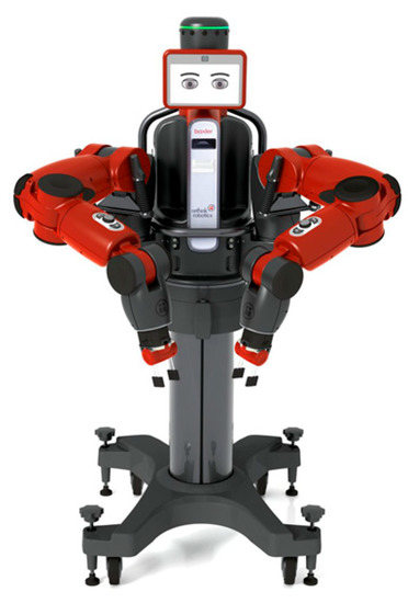
Figure 1. Baxter Robot.

4. Baxter Manipulator Kinematics

The Baxter Research Robot has two identical seven-joint manipulator arms. The coordinate frames and Denavit–Hartenberg [4] standard parameters convention used in [18] for manipulator kinematics computation were adopted in this paper. The resulting Denavit–Hartenberg parameters are shown in Table 1.

Table 1. Denavit–Hartenberg parameters.

i	${\mathit{\alpha }}_{\mathit{i}-1}$	${\mathit{a}}_{\mathit{i}-1}$	${\mathit{d}}_{\mathit{i}}$	${\mathit{\theta }}_{\mathit{i}}$
1	0	0	$L_0$	${\theta }_1$
2	−90°	$L_1$	0	${\theta }_2$+ 90°
3	90°	0	$L_2$	${\theta }_3$
4	−90°	$L_3$	0	${\theta }_4$
5	90°	0	$L_4$	${\theta }_5$
6	−90°	$L_5$	0	${\theta }_6$
7	90°	0	$L_6$	${\theta }_7$
EE	90°	0	$L_6$$+L_7$	$\theta$7

where

$L_0$ = 281.35 mm	$L_4$ = 374.29 mm
$L_1$ = 125 mm	$L_5$ = 10 mm
$L_2$ = 364.35 mm	$L_6$ = 229.525 mm
$L_3$ = 69 mm	$L_7$ = 100 mm

The homogeneous transformation matrix from frame {i} to frame {i − 1} is given as follows:

$${}_i{}^{i-1}T=\left[\begin{array}{cccc}c{\theta }_i& -s{\theta }_i& 0& a_{i-1}\\ s{\theta }_{i}c{\alpha }_{i-1}& c{\theta }_{i}c{\alpha }_{i-1}& -s{\alpha }_{i-1}& -s{\alpha }_{i-1}{d}_i\\ s{\theta }_{i}s{\alpha }_{i-1}& c{\theta }_{i}s{\alpha }_{i-1}& c{\alpha }_{i-1}& c{\alpha }_{i-1}{d}_i\\ 0& 0& 0& 1\end{array}\right]$$

(4)

where

$c{\theta }_i=\cos \left({\theta }_i\right)$	$s{\theta }_i=\sin \left({\theta }_i\right)$
$c{\alpha }_{i-1}=\cos \left({\alpha }_{i-1}\right)$	$s{\alpha }_{i-1}=\sin \left({\alpha }_{i-1}\right)$

The end effector frame {7} to the base frame {0} homogeneous transformation matrix can be computed by:

$${}_7{}^{0}T={}_1{}^{0}T{}_{ 2}{}^{1}T{}_{ 3}{}^{2}T{}_{ 4}{}^{3}T{}_{ 5}{}^{4}T{}_{ 6}{}^{5}T{}_{ 7}{}^{6}T$$

(5)

The matrix ${}_7{}^{0}T$ is a function of the joint angles ${\theta }_1,{\theta }_2,\cdots ,{\theta }_7$ and has the form [18]:

$${}_7{}^{0}T=\left[\begin{array}{cc}{}_7{}^{0}R& {}_{}{}^0\overrightarrow{P}{}_{EE}\\ \underset{\_}{0}& 1\end{array}\right]$$

(6)

where ${}_7{}^{0}R$ is the rotation matrix from frame {7} to frame {0}, and ${}_{ }{}^0\overrightarrow{P}{}_{EE}$ is the position vector of the end effector in frame {0}.

The end-effector pose $X_i$ of the particle $i$ can be constructed from the components of ${}_7{}^{0}T$:

$$X_i={\left[{}_{ }{}^0\stackrel{\rightharpoonup }{P}{}_{EE}^T \left[q_0 q_1 q_2 q_3\right]\right]}^T$$

(7)

where $\left[q_0 q_1 q_2 q_3\right]$ is the quaternion equivalence of ${}_7{}^{0}R$.

The time rate of change of $X_i$ is then:

$$V_i={\left[{}_{}{}^0\dot{\overrightarrow{P}}{}_{EE}^T\left[{\dot{q}}_0{\dot{q}}_1{\dot{q}}_2{\dot{q}}_3\right]\right]}^T={\left[{}_{}{}^0\overrightarrow{V}{}_{EE}^T\left[{\dot{q}}_0{\dot{q}}_1{\dot{q}}_2{\dot{q}}_3\right]\right]}^T$$

(8)

which can be converted to joint rates of particle $i$ using the following relationships [18,19,20,21]:

$${}_{}{}^0\overrightarrow{\omega }{}_{EE}^{}=2\left[\begin{array}{cccc}-q_1& q_0& -q_3& q_2\\ -q_2& q_3& q_0& -q_1\\ -q_3& -q_2& q_1& q_0\end{array}\right]\left[\begin{array}{c}\dot{q_0}\\ \dot{q_1}\\ \dot{q_2}\\ \dot{q_3}\end{array}\right]$$

(9)

$${\dot{\mathbf{\theta }}}_{\mathbf{i}}={\left[{\dot{\theta }}_1{\dot{\theta }}_2{\dot{\theta }}_3{\dot{\theta }}_4{\dot{\theta }}_5{\dot{\theta }}_6{\dot{\theta }}_7\right]}^T={\mathit{J}}^T{\left(\mathit{J}{\mathit{J}}^T\right)}^{-1}\left[\begin{array}{c}{}_{}{}^0\overrightarrow{V}{}_{EE}^{}\\ {}_{}{}^0\overrightarrow{\omega }{}_{EE}^{}\end{array}\right]$$

(10)

where ${}_{ }{}^0\overrightarrow{\omega }{}_{EE}^{ }$ is the angular velocity of the end effector relative to frame {0} and $\mathit{J}$ is the Jacobian matrix of the manipulator [18,19,20,21].

5. Baxter Inverse Kinematics

The PSO algorithm (shown in Figure 2) to solve the inverse kinematics of the Baxter manipulator arm was implemented in MATLAB and is described below.

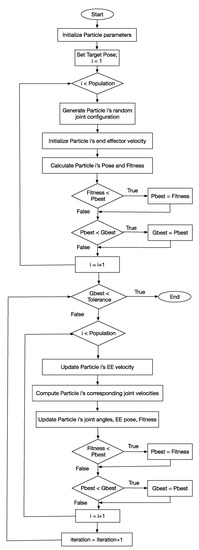
Figure 2. Flowchart of the PSO implementation.

The solution to the inverse kinematics problem is the set of joint angles of the particle with the final global best fitness function.

Experiment: Target Pose is Baxter’s left arm end effector pose when the arm is at the default untuck configuration. Three runs were performed with 60 particles, which yielded three different sets of solution joint angles corresponding to this Target Pose. This result was expected, since Baxter’s arm has seven joints (kinematically redundant); thus, the number of possible solutions is infinite. The Baxter robot (shown in Figure 1 was used to test all obtained results via our algorithm at the University of Houston Clear Lake Robotics and Control Laboratory. The Baxter robot arms have a default joint configuration called “untuck” where the arms are deployed and ready to run applications. After adjusting the untuck joint angle values using our results, a python program was run to move the robot’s left arm into the untucked position. All communications between the robot and the python code are established using Linux Ubuntu 16.04 and the Robot Operating System software framework. More details can be found in Fairchild and Harman [22].

Table 2 documents the solution joint angles and corresponding final end-effector pose for the three runs. Figure 3 and Figure 4 illustrate how quickly the inverse kinematics solution converges for run 1, after roughly 100 iterations. Although not shown here due to space limitation, runs 2 and 3 have similar speeds of convergence. Figure 5 shows the global best fitness function for run 1, and Figure 6 shows the three Baxter left-arm configurations corresponding to the three different sets of solution joint angles from the three runs.

Table 2. Results of three runs with Target Pose at Baxter’s Untuck Configuration.

	Run 1 Solution	Run 2 Solution	Run 3 Solution
Joint angles (degrees) $\left[\begin{array}{c}{\theta }_1\\ {\theta }_2\\ {\theta }_3\\ {\theta }_4\\ {\theta }_5\\ {\theta }_6\\ {\theta }_7\end{array}\right]$	$\left[\begin{array}{c}-68.401\\ -77.656\\ 25.576\\ 120.917\\ 173.673\\ -44.975\\ -157.931\end{array}\right]$	$\left[\begin{array}{c}-101.024\\ -21.994\\ 90.5023\\ 110.675\\ 108.897\\ -80.278\\ -110.091\end{array}\right]$	$\left[\begin{array}{c}-5.6836\\ 17.4950\\ -116.247\\ 113.035\\ 101.1241\\ 120.000\\ -49.540\end{array}\right]$	Default Untuck Joint angles $\left[\begin{array}{c}-4.5837\\ -57.2958\\ -68.182\\ 111.153\\ 38.388\\ 59.014\\ -28.647\end{array}\right]$
Final pose $\left[\begin{array}{c} {}_{ }{}^{0}p{}_{EEx}\\ {}_{ }{}^{0}p{}_{EEy}\\ {}_{ }{}^{0}p{}_{EEz}\\ q_0\\ q_1\\ q_2\\ q_3\end{array}\right]$	$\left[\begin{array}{c}0.5758\\ 0.1770\\ 0.2605\\ 0.0255\\ 0.1408\\ 0.9896\\ 0.0116\end{array}\right]$	$\left[\begin{array}{c}0.5758\\ 0.1770\\ 0.2605\\ 0.0255\\ 0.1408\\ 0.9896\\ 0.0116\end{array}\right]$	$\left[\begin{array}{c}0.5758\\ 0.1770\\ 0.2605\\ 0.0255\\ 0.1408\\ 0.9896\\ 0.0116\end{array}\right]$	Target Pose $X_T$ $\left[\begin{array}{c}0.5758\\ 0.1770\\ 0.2605\\ 0.0255\\ 0.1408\\ 0.9896\\ 0.0116\end{array}\right]$

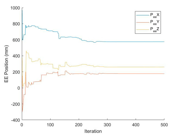
Figure 3. Plot of run 1 EE position.

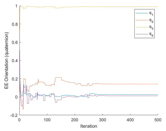
Figure 4. Plots of run 1 EE orientation.

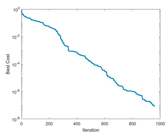
Figure 5. Best cost (fitness function) for run 1.

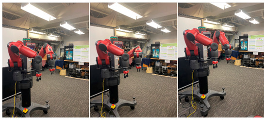
Figure 6. Baxter’s left-arm in joint configurations of runs 1, 2 and 3 (in left to right order).

From Figure 6, it is clear that the Baxter left−arm end−effector pose is the same even though the three different sets of joint angles are completely different. This is due to the inherent kinematic redundancy of the seven-joint Baxter arm and the randomness of the initial configuration of the swarm joint angles. The next paragraph will address how a more customized solution can be obtained for Baxter and other kinematically redundant manipulator arms.

It must be emphasized that our approach to solving the inverse kinematics for serial robotic manipulators can be applied to manipulators with any number of joints and not restricted to just seven. In the case of manipulators with kinematic redundancy (seven or more joints in six-dimensional space), the algorithm can easily be manipulated to obtain certain desirable solutions by simple modifications such as adding the joint angle error from its desired value for any number of joints to the calculation of particle i’s fitness function $f_i$, i.e.,

$$f_i={\sqrt{{\displaystyle \sum }_{j=1}^7{\left(X_{Tj}-X_{ij}\right)}^2+{\displaystyle \sum }_k{\left({\theta }_k^{des}-{\theta }_{ik}\right)}^2}}_{ }$$

(11)

where ${\theta }_k^{des}$ is the desirable value of joint angle k in the solution of the inverse kinematics problem. As an example, another run was made setting the desired value of the 6th joint to ${\theta }_6^{des}=59.014$ deg, which corresponds to that of the default untuck configuration. For this run, the final joint configuration is that of the default untuck configuration as shown below, although the speed of convergence is slower than when the 6th joint is not constrained to a desired value.

Target joint angles in degrees:

[−4.584  −57.296  −68.182  111.154  38.388  59.014  −28.6479]

Final joint angles in degrees (Figure 7):

[−4.5837  −57.2958  −68.1820  111.1538  38.3882  59.0147  −28.6479]

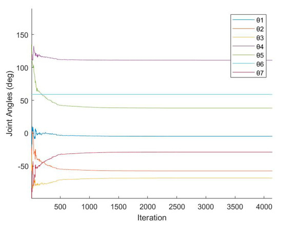
Figure 7. Baxter’s left−arm joint angles in the default untuck joint configuration obtained by setting ${\theta }_k^{des }$ = 59.014°.

6. Parallel Processing of the PSO Algorithm

The results described in the previous section were obtained with the inverse kinematics algorithm implemented using MATLAB, a mathematically convenient but not necessarily a time efficient language for this type of problem. In an effort to improve the speed of execution, the algorithm was implemented using Portable Operating Interface (POSIX) threads, commonly called pthreads which are executed in parallel. Idealistically, if there are enough processors, each particle dynamic computation can be programmed into one pthread which runs on one processor. A variety of test runs were performed using a laptop computer with 21 processors to evaluate the speed of convergence as shown in Table 3 and Table 4. The parallel processing flowchart is shown in Figure 8. A brief description of the POSIX threads pseudo code is given below.

Table 3. One particle per thread.

	Target 1	Target 2	Target 3
Number of particles	20	20	20
Threads	20	20	20
Convergence time (s)	0.028	0.033	0.028
Cost (meter)	6.73 × 10−5	8.94 × 10−5	8.26 × 10−5

Table 4. Three particles per thread.

	Target 1	Target 2	Target 3
Number of particles	60	60	60
Threads	20	20	20
Convergence time (s)	0.039	0.034	0.046
Cost (meter)	8.42 × 10−5	8.27 × 10−5	7.33 × 10−5

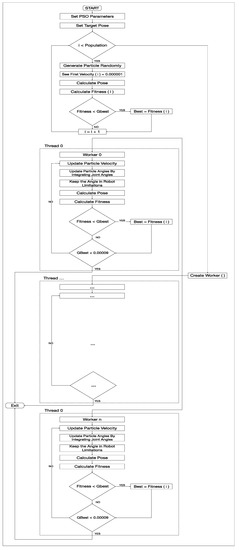
Figure 8. PSO implementation in threads.

Posix Threads

A thread API based on standards for C/C++ is provided by the POSIX thread libraries. A new concurrent process flow may be spawned using it. It works best with systems that have several processors or cores, since the process flow can be scheduled to run on a different processor, allowing for parallel or distributed processing to speed up the system.

Each thread has a unique:

• Thread ID
• Set of Registers, Stack Pointer
• Stack for local variables, return addresses
• Signal mask
• Priority
• Return value

Note: Pthread functions return “0” if OK.

• x = Set number of threads
• p = Set number of Particles
• function PSO_calculation(*thread_id):
•  instantiate tid as a long
•  tid = cast thread_id to long
• while GlobalBestCost > 0.00009 do
•  PSO iteration
• endwhile
•  exit thread with NULL
• endfunction

• function create_threads ():
• instantiate threads as array of NUM_THREADS pthread_t objects
• instantiate attributes object pthread_attr
• set stat to null pointer.
• initialize thread attributes object attr.
• set detach state of attr to joinable.
•  for i from 0 to NUM_THREADS do
•  create a worker thread with pthread_create, using thread[i] as thread ID, attr as thread attributes, PSO_function() as start routine, passing thread ID data argument as needed.
•   if the pthread_create() function returns an error code:
•    Print output “Failed to create worker thread.”
•    exit program.
•   endif
•  endfor
• endfunction

Threads were created according to the population of our swarm. In this research, all 20 cores of an I9 processor were used to create an array of 20 threads with different particle numbers as 20, 60 and 100. The following parameters in the function were used to generate threads:

&Threads[i]: pointer to an unsigned integer value that returns the thread id of the thread created.

&attr: You can specify behavior that differs from the default by using attributes. An attribute object may be specified during thread creation with a pointer to a structure that is used to define thread attributes such detached state, scheduling policy, and stack address. If attributes are set to NULL, threads use the default settings, which are generally adequate.

PSO calculation: the pointer to the function to be threaded in our case is PSO_calculation.

void *i: pointer to void that contains the arguments to the function defined in the earlier argument.

• function destroy_threads ():
• Destroy the thread attributes object created earlier in the program.
• for i from 0 to NUM_THREADS do
•   Wait for the worker thread to complete before continuing execution.
•   if pthread_join returns error:
• Print output (“error message)
• exit (−1)
•  else:
•   Print output “that all worker threads have completed before the program exits.”
•   Print output “Ending Status of Thread.”
•  endif
• endfor
• endfunction

The computational process waits for each thread to finish its current task. When all threads have finished their work, i.e., have obtained a satisfying error value, the software terminates all the threads and goes back to the main function.

It must also be emphasized that in taking advantage of the parallel processing implementation, it was found that instead of waiting for the completion of all particle dynamics computations at the end of each iteration before determining the global best fitness value Gbest, the PSO algorithm converges significantly faster (more than an order of magnitude) by letting each particle update the Gbest as it finishes its computations. Figure 9 and Figure 10 reflect the contribution and motion of the particle computation threads, respectively. In Figure 9, the color circles represent the Gbest value of the particles while in Figure 10, they represent the end-effector pose of the particles during the solution process. Figure 11 shows a close−up view of the particles arriving at the target solution.

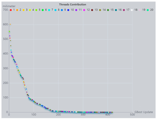
Figure 9. Threads contribution to GBest determination.

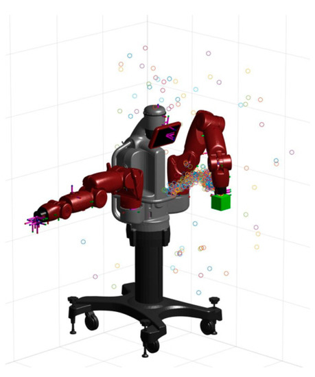
Figure 10. Motion of the particle swarm.

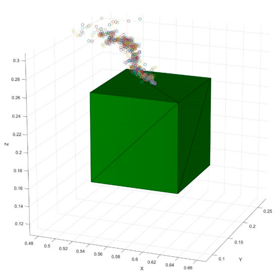
Figure 11. Particles arriving at solution (close−up).

7. Results and Future Work

Table 5 shows the comparison in particle swarm size, number of iterations, convergence time, end effector space degrees of freedom, joint space degrees of freedom and accuracy between our PSO algorithm and those of references [3,12].

Table 5. Comparison of our algorithm with other swarm intelligence methods.

Paper	Particle/Iteration	Time (ms)	Algorithm	Dimension	Accuracy (mm|RD)
Dereli [3]	300/500	449.8	PSO	[Position]	67.1 × 10−3
Dereli [3]	100/500	444.1	ABC	[Position]	54.7 × 10−4
Dereli [3]	50/500	920.4	Firefly	[Position]	65.0 × 10−5
Dereli [3]	150/500	231.9	QPSO	[Position]	27.7 × 10−17
Starke [12]	NA	22	HGSA	[Position, Orientation]	1.00
Starke [12]	NA	30–600	PSO	[Position]	1.00
Starke [12]	NA	50–500	GA	[Position]	1.00
Our Algorithm	20/NA	18–40	PSO	[Position, Orientation]	<0.09

Several algorithms have been created for the issue of inverse kinematics, and each one has been fine for its particular need. As a result, it is challenging to undertake a qualitative comparison that considers all performance factors. In addition, few cited studies specify the execution time. Table 5 contrasts our technique with other strategies used by researchers to solve inverse kinematics among those who had included execution time. Dereli [3] solely concentrates on converging position values, as shown in Table 5, and finds that after 500 iterations with 0.1 mm accuracy, the average execution time varies between 230 and 930 milliseconds depending on the optimization technique. Dereli [3] claims that PSO is the second-worst optimization in terms of time for tackling only 3-dimensional objectives (Px, Py, Pz). On the other hand, our method using the POSIX thread with full (Position, Orientation) convergence only requires 18–40 milliseconds with a precision of less than 0.1 mm. The number of iterations is irrelevant because our approach is based on independent particles.

Nonetheless, it may be possible to calculate the average number of updates made by each particle. Hence, even in the search for 7-dimensional space [Px, Py, Pz, q0, q1, q2, q3], Table 4 and the comparison Table 5 demonstrate that the performance of our algorithm is faster and could establish more calculations in a shorter amount of time. Starke [12] suggests that a heuristic hybridization of GA and PSO can achieve much more efficiency than the individual methods and still be a general and all-encompassing strategy for resolving the inverse kinematics problem. Starke [11] believes his method is practical for various real-time applications. Our POSIX threads implementation demonstrated faster computation times with more accuracy using one technique. The originality of our algorithm, which is moving the particles independently without waiting for the previous particle, increased the algorithm’s performance and decreased the computation time.

Nevertheless, combining Starke’s [11] approach and our method may improve efficiency, robustness and reliability. Since the I9 processor only has 20 cores, testing could only be done with 20 threads. Since our approach applies to a limitless number of threads, theoretically, the speed of convergence for our approach is only limited by the number of available computer processors that can run in parallel. Our future work will be to continue testing our algorithm with better computing equipment that is accessible to us.

8. Conclusions

Many robotic manipulator inverse kinematics solvers use swarm intelligence to find the set of joint angles that will achieve the predetermined end-effector’s position or orientation. However, one of the challenges remaining is that they are not capable of finding the position and orientation simultaneously. In addition, there is room for improvement in terms of speed and efficiency, as many of these methods can be slow to find the correct sets of intersegmental angles that will place the end effector in the given position and orientation. Therefore, to solve the inverse kinematics for serial robotic manipulators, a Particle-Swarm-Optimization-based technique is applied in conjunction with the Portable Operating Interface (POSIX) threads to take advantage of the independent swarm particle dynamics.

The novelty of our approach is that it offers a comprehensive solution for both the position and orientation of the robot end effector. The calculation of the Baxter robot manipulator inverse kinematics in C++ code could be parallelized using the POSIX threads library. It was also demonstrated that it is possible to obtain fast converge, with results in < 50 msec for the Baxter robot’s 7-joint manipulator arm when particle swarm optimization is programmed using POSIX threads. By only using the global and local best known, each particle (thread) performs as decentralized in the search area without waiting for others. Our study shows that the PSO method converges efficiently in < 50 msec by allowing each particle to update the global best as it completes its computations. The convergence time results (Table 3 and Table 4) were obtained with our limited computing power equipment: a laptop computer with an Intel Core i9-12900H 2.50 GHz Processor (14-Cores, 20-Threads). In future applications with more powerful computing equipment, better convergence timing is expected with our parallel processing algorithm of the PSO.

References

- Kennedy, J.; Eberhart, R. Particle Swarm Optimization. In Proceedings of the IEEE International Conference on Neural Networks, Perth, Australia, 27 November–1 December 1995. [Google Scholar]
- Kennedy, J. The particle swarm: Social adaptation of knowledge. In Proceedings of the IEEE International Conference on Evolutionary Computation, Indianapolis, IN, USA, 13–16 April 1997. [Google Scholar]
- Dereli, S.; Köker, R. A meta-heuristic proposal for inverse kinematics solution of 7-DOF serial robotic manipulator: Quantum behaved particle swarm algorithm. Artif. Intell. Rev. 2020, 53, 949–964. [Google Scholar] [CrossRef]
- Denavit, J.; Hartenberg, R.S. A kinematic notation for lower-pair mechanisms based on matrices. Trans. ASME J. Appl. Mech. 1955, 23, 215–221. [Google Scholar] [CrossRef]
- Corke, P. Robotics, Vision and Control—Fundamental Algorithms in MATLAB; Springer: Berlin/Heidelberg, Germany, 2011. [Google Scholar]
- Huang, H.C.; Chen, C.P.; Wang, P.R. Particle swarm optimization for solving the inverse kinematics of 7-DOF robotic manipulators. In Proceedings of the 2012 IEEE International Conference on Systems, Man, and Cybernetics (SMC), Seoul, Republic of Korea, 14–17 October 2012; pp. 3105–3110. [Google Scholar]
- Durmuş, B.; Temurtaş, H.; Gün, A. An inverse kinematics solution using particle swarm optimization. In Proceedings of the International Advanced Technologies Symposium, Elazig, Turkey, 16–18 May 2011; Volume 4, pp. 193–197. [Google Scholar]
- Ayyildiz, M.; Cetinkaya, K. Comparison of four different heuristic optimization algorithms for the inverse kinematics solution of a real 4-DOF serial robot manipulator. Neural Comput. Appl. 2016, 27, 825–836. [Google Scholar] [CrossRef]
- Sancaktar, I.; Tuna, B.; Ulutas, M. Inverse kinematics application on the medical robot using adapted PSO method. Eng. Sci. Technol. Int. J. 2018, 21, 1006–1010. [Google Scholar] [CrossRef]
- Rokbani, N.; Alimi, A.M. IK-PSO, PSO Inverse Kinematics Solver with Application to Biped Gait Generation. arXiv 2012, arXiv:1212.1798. [Google Scholar]
- Rokbani, N.; Alimi, A.M. Inverse kinematics using particle swarm optimization, a statistical analysis. Procedia Eng. 2013, 64, 1602–1611. [Google Scholar] [CrossRef]
- Starke, S.; Hendrich, N.; Magg, S.; Zhang, J. An efficient hybridization of genetic algorithms and particle swarm optimization for inverse kinematics. In Proceedings of the 2016 IEEE International Conference on Robotics and Biomimetics (ROBIO), Qingdao, China, 3–7 December 2016; pp. 1782–1789. [Google Scholar]
- Nguyen, L.A.; Danaci, H.; Harman, T.L. Inverse Kinematics For Serial Robot Manipulator End Effector Position And Orientation By Particle Swarm Optimization. In Proceedings of the 2022 26th International Conference on Methods and Models in Automation and Robotics (MMAR), Międzyzdroje, Poland, 22–25 August 2022; pp. 288–293. [Google Scholar] [CrossRef]
- Kucuk, S. Energy minimization for 3-RRR fully planar parallel manipulator using particle swarm optimization. Mech. Mach. Theory 2013, 62, 129–149. [Google Scholar] [CrossRef]
- Beeson, P.; Ames, B. TRAC-IK: An Open-Source Library for Improved Solving of Generic Inverse Kinematics; Supported by NASA Contracts NNX14CJ19P & NNX15CJ06C; TRACLabs Inc.: Webster, TX, USA, 2015. [Google Scholar]
- Diankov, R.; Kuffner, J. OpenRAVE: A Planning Architecture for Autonomous Robotics; CMU-RI-TR-08-34; Carnegie Mellon University: Pittsburg, PA, USA, 2008. [Google Scholar]
- Rethink Robotics, Inc. Baxter Research Robot: Technical Specification Datasheet & Hardware Architecture Overview; Rethink Robotics, Inc.: Bochum, Germany, 2016. [Google Scholar]
- Craig, J. Introduction to Robotics: Mechanics and Control, 4th ed.; Wiley: Hoboken, NJ, USA, 2018. [Google Scholar]
- Wittenburg, J. Dynamics of Systems of Rigid Bodies; B.G. Teubner Stuttgart: Stuttgart, Germany, 1977. [Google Scholar]
- Nguyen, L.A.; Le, K.; Harman, T.L. Kinematic Redundancy Resolution For Baxter Robot. In Proceedings of the International Conference on Automation, Robotics and Applications, Prague, Czech Republic, 4–6 February 2021. [Google Scholar]
- Yoshikawa, T. Analysis and Control of Robotics Manipulators with Redundancy. In Robotics Research: First International Symposium; Brady, M., Paul, R., Eds.; MIT Press: Cambridge, MA, USA, 1984. [Google Scholar]
- Fairchild, C.; Harman, T.L. ROS Robotics by Example, 2nd ed.; Packt Publishing: Birmingham, UK, 2017. [Google Scholar]
Disclaimer/Publisher’s Note: The statements, opinions and data contained in all publications are solely those of the individual author(s) and contributor(s) and not of MDPI and/or the editor(s). MDPI and/or the editor(s) disclaim responsibility for any injury to people or property resulting from any ideas, methods, instructions or products referred to in the content. |
© 2023 by the authors. Licensee MDPI, Basel, Switzerland. This article is an open access article distributed under the terms and conditions of the Creative Commons Attribution (CC BY) license (https://creativecommons.org/licenses/by/4.0/).