Article

Stain Defect Classification by Gabor Filter and Dual-Stream Convolutional Neural Network

1
Industrial AI Research Center, Chungbuk National University, Cheongju 28644, Republic of Korea
2
System Engineering MEga Solution (SEMES), Cheonan 31040, Republic of Korea
3
Department of Intelligent Systems and Robotics, Chungbuk National University, Cheongju 28644, Republic of Korea
*
Author to whom correspondence should be addressed.
These authors contributed equally to this work.
Appl. Sci. 2023, 13(7), 4540; https://doi.org/10.3390/app13074540
Submission received: 6 March 2023 / Revised: 21 March 2023 / Accepted: 1 April 2023 / Published: 3 April 2023
(This article belongs to the Section Robotics and Automation)

Abstract

:
A stain defect is difficult to detect with the human eye because of its characteristic of having a very minimal difference in brightness with the local area of the surface. Recently, with the development of Deep learning, the Convolutional Neural Network (CNN) based stain defect classification method has been proposed. This paper proposes a Dual-stream CNN for stain defect classification using a Gabor filter image. Using Dual-stream structure CNN, Gabor filter images and Gray image (Original) preserve their respective features. The experiment based on the Magnetic Tile (MT) stain data set and the Compact Camera Module (CCM) stain dataset confirms that the proposed method has an improved performance based on the precision, recall, and F1-score in comparison to the Single-stream extraction-based method. Gabor filter images have an advantage in image texture analysis and can be used as an input to the CNNs. The Dual-stream structure better extracts the features needed for classification.

1. Introduction

Detecting a stain defect image is challenging because the ambiguous boundary of a stain defect with an image processing–based method is complex. A stain defect is caused by an error in the manufacturing process, such as external contaminants, uneven paint coating, and other errors. It is slightly bright or has a dark brightness in contrast to a local area, and this contrast is difficult to detect with the naked eye.
Previous stain defect detection studies have detected stain defects using image processing techniques [1,2,3,4,5,6,7]. Kong et al. [1] proposed a method for calculating the variance of the inspection area image and judging it as a stain defect when it exceeds a certain threshold. Zhang et al. [3] detected the stain defect by calculating the Just Noticeable Difference (JND) value after applying the watershed method in the forward and reverse directions of the image to detect the boundary of the stain defect area. Han and Shi [6] extracted the wavelet image of an input image using wavelet transform and detected a stain defect by removing the background component with the difference image between the wavelet image and the input image. The above methods are methods for modeling and removing the background component and have a disadvantage in that accurate modeling of the background component is required.
A study using the Gabor filter to detect stain defects has been proposed to solve this shortcoming [8,9,10,11]. The Gabor filter was presented as a human visual system model and as a filter that extracts texture features using a sine wave with a specific frequency and direction. The Gabor filter detected and modeled the texture feature of the background component having the same continuous pattern and was used to detect the stain defect by removing the background component of the input image. Bi et al. [8] extracted the Gabor filter image using the Gabor filter’s actual part and created a binarized image based on a specific threshold to detect the stain defect on the liquid crystal display (LCD). Mao et al. [10] selected Gabor filter parameters with high stain defect classification performance by applying them to the training image. The stain defect was then detected using the selected Gabor filter.
Recently, with the development of deep learning, several studies to detect defects using a CNN have been proposed [12,13,14,15,16,17,18,19,20,21,22,23,24]. Xiao et al. [12] proposed a hierarchical feature–based CNN (H-CNN) structure that generates Regions Of Interest (ROI) using region-based CNN (R-CNN) and detects the defect using a fully CNN (F-CNN). Singh et al. [14] compared the classification performance for stain defects on metal surfaces using a CNN such as ResNet [25] and YOLO [26]. Yang et al. [15] created a defect detection model by learning stain defects using the transfer learning technique of a deep CNN extractor trained in advance on the ImageNet Large Scale Visual Recognition Challenge 2012 (ILSVRC2012) dataset. Hou et al. [24] proposed a directional kernel to detect weak scratches.
The segmentation method can accurately explore the shape of the defect, but it takes a long time to compute. In addition, several studies to detect defects using segmentation have been proposed [27,28,29]. Tabernik [27] proposed After applying segmentation, the defect was detected using the method using the detection. In addition, Huang [28] introduced The MT set first, and defects were detected using the McuePushU network.
The previous deep learning–based stain defect classification method used a single inspection image as input [14,15]. The Gabor filter image has an advantage in image texture analysis, so performance improvement is expected when used as an input for CNN. However, it is necessary to design a CNN to extract features advantageous for stain defect classification using different domains, such as inspection and Gabor filter images.
This paper proposes a CNN for stain defect classification using inspection images and Gabor filter images intending to improve the performance of stain defect classification. First, a Gabor filter image is created using a Gabor filter on the inspection image obtained from the camera. A GLCM is constructed for the Gabor filter image, and an IDM value, a local homogeneity feature, is extracted from GLCM. The Gabor filter image is selected based on the IDM, and the inspection image and the selected Gabor filter image are used as input to the CNN.
The contribution of this paper is as follows.
1. Gabor images with Gabor filters applied were used to improve the accuracy of stain defect detection. A method of adding features for spot detection using Gabor images was used rather than a method without Gabor filter images. It was confirmed through experiments that the method using the Gabor image improved the accuracy.
2. The stain defect classification performance was improved through a Dual-stream extraction based on inspection image and Gabor filter images, compared to the existing Single-stream extraction. The most suitable image for stain defect classification from the extracted Gabor filter image was selected and used as an input to a Dual-stream extraction that connects two streams in parallel. Through this, the features of each input image were extracted independently and merged in a fully connected layer to improve the stain defect classification accuracy.
This paper is structured as follows. Section 2 describes the structure of the stain defect classification system proposed in this paper. Section 3 describes the Gabor filter image creation and selection process. Section 4 describes the structure of a Single-stream extraction and a Dual-stream extraction. Section 5 demonstrates the performance of the proposed method, the Dual-stream extraction, by conducting experiments on the MT and CCM datasets. Lastly, Section 6 describes the conclusion of this paper and future research.

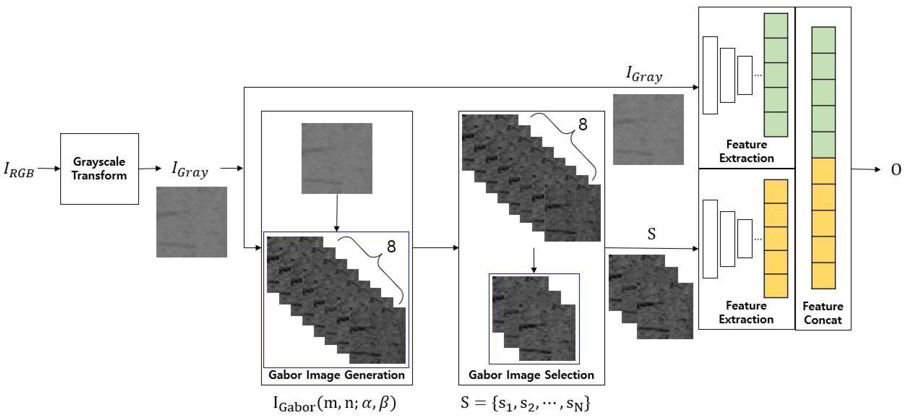
2. Stain Defect Classification System

The structure of the stain defect classification system proposed in this paper is shown in Figure 1. The proposed method comprises gray-scale transform, Gabor image generation, Gabor image selection, and CNN. The general process is as follows. The input inspection image I R G B is converted to a gray-scale inspection image I G r a y through gray-scale transform. After this, the Gabor image was generated and selected from the input image. Finally, the classification result O was obtained using a CNN with the selected Gabor images and gray-scale inspection image.
Let R m n , G m n , and  B m n are red channel, green channel, and blue channel of the image, respectively, while M and N are the height and width of the image, respectively.
I RGB = i 11 i 12 i 1 N i 21 i 22 i 2 N i M 1 i M 2 i M N w h e r e , i m n R m n G m n B m n i m n R 1 X 3 ( m = 1 , , M , n = 1 , , N )
I G r a y can be obtained as follows.
I Gray = j 11 j 12 j 1 N j 21 j 22 j 2 N j M 1 j M 2 j M N w h e r e , j m n = 0.229 R m n + 0.587 G m n + 0.114 B m n 3 j m n R 1 X 1 ( m = 1 , , M , n = 1 , , N )
The Gabor image generation step is a step to obtain the Gabor filter image G k for each phase. The Gabor filter transform uses a complex kernel with real and imaginary parts.
G = G ( k ) | k = 1 , 2 , , K
In the Gabor filter image selection step, a Gabor filter image with features useful for stain defects is selected among the generated Gabor filter images. By inputting the gray-scale inspection image I G r a y and the selected Gabor filter image G ´ into the CNN E , the classification result O for the inspection image is the output.
O = E ( I G r a y , G ´ )

3. Gabor Image from Stain Defect Image

Gabor filter is used for image processing for reasons like how the human visual system responds. Gabor filter is a Gaussian filter modulated by a sine function. The Gabor filter image is the result of a convolution operation between the Gabor filter and the image. Because the Gabor filter can acquire the result according to the direction and frequency, it is possible to check what features exist in the input image in a specific direction and frequency band.
Let x and y be the pixel coordinates of the Gabor filter. Gabor filter can be defined as the following equation. σ is a variable that determines the width of the Gabor filter kernel. λ is a variable that determines the addition/subtraction period of the Gabor filter kernel. θ is a variable that determines the direction of the Gabor filter kernel, and ψ is a mobility variable of the filter. γ is a variable for adjusting the horizontal and vertical ratio of the filter. Lastly, x and y are the x and y coordinates of the Gabor filter rotated by θ , respectively.
g ( x , y ; λ , θ , ψ , σ , γ ) = exp ( x 2 + γ 2 y 2 2 σ 2 ) cos ( 2 π x λ + ψ ) w h e r e , x = x cos θ + y sin θ y = x sin θ + y cos θ
Gabor filter can obtain various result values according to internal parameters. Among these results, to select an image to improve the stain defect classification performance, the GLCM and the Haralick texture feature based on it were used. GLCM transformation is an algorithm that transforms two neighboring pixel values in an image into spatial coordinates of an M × N matrix. Let the Δm and Δn are offsets in the width and height directions, respectively. the GLCM result matrix C Δ m , Δ n can be defined as follows.
C Δ m , Δ n ( i , j ) = m = 1 M n = 1 N = 1 i f   I G r a y ( m , n ) = i a n d I G r a y ( m ´ , n ´ ) = j 0 o t h e r w i s e w h e r e , m ´ = m + Δ m n ´ = n + Δ n
The GLCM matrices for 0 , 45 , 90 , and  135 directions can be obtained, respectively, according to the Δm and Δn. The Δm and Δn values for each angle are respectively (0,1), (1,0), (−1,1), (−1,−1). As the stain defect has an unspecified texture, features for all four directions should be used. Therefore, the GLCM matrix for four directions was obtained, and then the average value was used. The average matrix P for the GLCM can be calculated as follows.
P = C 0 , 1 + C 1 , 0 + C 1 , 1 + C 1 , 1 4
This paper used the Inverse Difference Moment (IDM) feature, one of the Haralick texture features, as a selection criterion for the generated Gabor filter image. IDM is an index indicating the local homogeneity of an image and it can be expressed as the following equation. Let W and H be the width and height of GLCM, respectively, and W and H have the same value (W = H).
I D M = i = 0 W j = 0 H P ( i , j ) 1 + ( i j ) 2
The IDM value was used to select the Gabor filter images for stain defect classification. The denominator of the IDM equation becomes 1 in the diagonal component of the GLCM, having the same brightness value as the neighboring pixels, and the IDM value becomes the maximum in the main diagonal section. Meanwhile, as the distance from the diagonal component of the GLCM increases, the denominator’s value rises, and the IDM value decreases. In other words, a large IDM value suggests the presence of multiple pixels having similar brightness, and a small IDM value means that there are many pixels with a difference between neighboring pixels. Therefore, the smaller the IDM value, the lower the local homogeneity in the image, and it can be said that the image has a relatively clear boundary of the stain defect.

3.1. Gabor Image Generation

To extract the stain defect features for various frequency bands and directional, a total of 64 Gabor filters are generated according to the 8 amplitudes λ α and eight phases θ β as shown in the following equation, respectively. The size of each Gabor filter is 3 × 3.
g ( x , y ; λ α , θ β , ψ , σ , γ ) = exp ( x 2 + γ 2 y 2 2 σ 2 ) cos ( 2 π x λ α + ψ ) w h e r e , x = x cos θ β + y sin θ β , y = x sin θ β + y cos θ β
λ α = 2 4 α + 2 2 , θ β = β 8 π w h e r e , α = 0 , 1 , , 7 , a n d β = 0 , 1 , , 7
Gabor filter image I G a b o r are created through convolution operation between I G r a y and Gabor filter created.
I G a b o r ( m , n ; α , β ) = x = 1 x = 1 y = 1 y = 1 g ( x , y ; λ α , θ β , ψ , σ , γ ) · I G r a y ( m + x , n + y )

3.2. Gabor Image Selection

Among the 8 Gabor images created in Section 3.1, N images with the smallest IDM value are selected. An image with a small IDM is an image with a large change in values between pixels. Efficient feature extraction for stain detection is possible using the selected Gabor image. The Gabor image selection steps consist of follows.
Step (1) For the Gabor image created in Section 3.1, create an average image I ´ G a b o r for each phase.
I ´ G a b o r ( m , n ; β ) = 1 7 α = 0 7 I G a b o r ( m , n ; α , β )
Step (2) Normalization is performed on the Gabor filter image I ´ G a b o r .
I ´ G a b o r ( m , n ; β ) = I ´ G a b o r ( m , n ; β ) min ( I ´ G a b o r ( m , n ; β ) ) max ( I ´ G a b o r ( m , n ; β ) ) min ( I ´ G a b o r ( m , n ; β ) )
Step (3) According to Equations (6) and (7), the Gabor filter image I G a b o r (m,n; β ) is transformed into a GLCM, and the average matrix P β is obtained.
Step (4) IDM feature values are extracted from each average matrix P β .
F = F β | F β = i = 0 W j = 0 H P β ( i , j ) 1 + ( i j ) 2 w h e r e , β = 0 , 1 , , 7
Step (5) The top N Gabor filter images with the highest IDM feature values are selected. The Gabor filter image selection Algorithm 1 proceeds as follows.
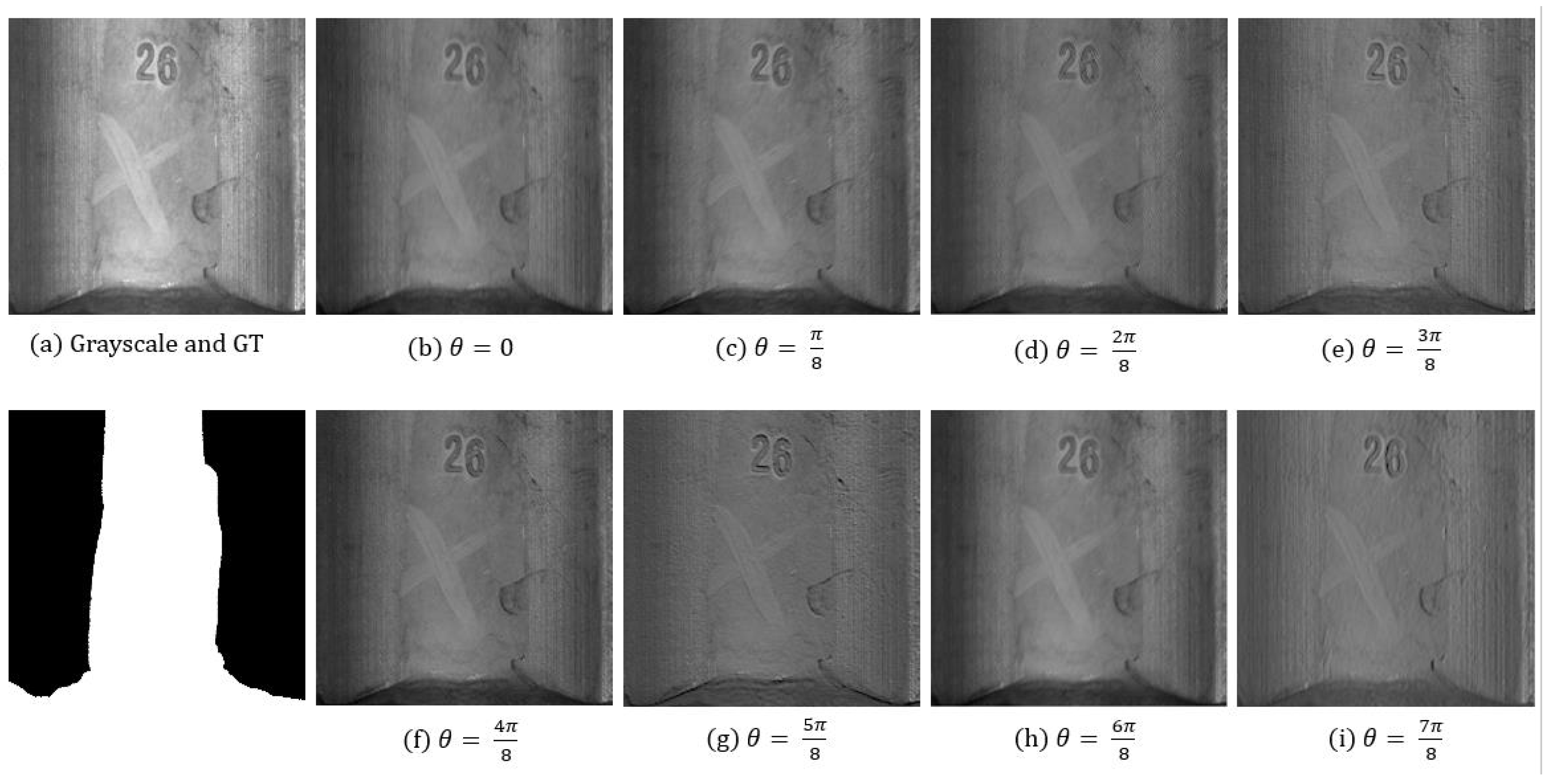
Figure 2 and Figure 3 show the Gabor filter images for each phase concerning the stain defect image generated on the MT dataset and CCM dataset. Figure 2a and Figure 3a are a gray-scale image for the inspection image, and it also is a ground truth image showing the location of the stain defect. Figure 2b–i and Figure 3b–i are Gabor filter images according to phase, selected for CNN model creation according to their IDM values. The clarity of the boundary difference between the stain defect and the non-defect one depends on the Gabor filter’s phase. In the MT dataset of Figure 2, the IDM values increase in the order of (b), (c), (h), (d), (f), (i), (e), and (g), and in the CCM dataset of Figure 3, the IDM values increase in the order of (b), (c), (d), (i), (f), (h), (e), (g) increase.
Algorithm 1 Select N Gabor filter image
  • Require: Gabor filter image I ´ G a b o r ( m , n ; β ) , IDM value F
  • Ensure: Selected Gabor filter image set S
  • S = 0
  • for S i z e ( S ) < N do
  •       γ = argmin β ( F )
  •       S I ´ G a b o r ( m , n ; γ )
  • end for

4. Feature Vector Extraction Based CNN

According to the previous process, the input of the CNN is a I G r a y and a set of Gabor filter images S = s 1 , s 2 , , s N . In general, CNN has one stream and uses a method of inputting a single image with N+1 channels by combining a gray-scale inspection image and a Gabor filter image. However, a Gabor filter image is generated through a Gabor filter and has a different domain from a gray-scale inspection image. When features are extracted from images of other parts with a CNN composed of a Single-stream, the process of extracting unique features that can be extracted from each part may not be performed smoothly. In this case, constructing a CNN with multiple streams to analyze the features of each part and then combining them can increase the detection accuracy. This section describes the structures of a Single-stream extraction and a Dual-stream extraction, respectively.

4.1. Single-Stream Extraction

Single-stream extraction is the most common type of CNN. Single-stream extraction is a structure that has been used in many CNNs, such as GoogLeNet. Single-stream extraction has a funnel-shaped structure in which layers are stacked and descended.
The CNN used in this paper was designed based on Res_Block in Figure 4 consisting of three convolution layers, is a method devised in Res Net [25] that uses the residual learning method. Res_Block simplifies the loss function with a shortcut structure between the input and output and is designed to alleviate the gradient vanishing problem that occurs when designing a deep CNN. The CNN used in this paper was designed based on Res_Block in Figure 4. Res_Block was applied to both Single-stream and Dual-stream extraction structures.
Figure 4 shows the structure of the Single-stream extraction used in this paper. The I M e r g e was constructed by stacking Gabor filter image N channels and gray-scale inspection images in parallel, and this I M e r g e is used as an input to CNN. A feature map with 64 channels was extracted through a convolution layer using a 7 × 7 kernel and sampled at a size of 112 × 112 using max pooling. After that, the feature map was extracted through 4 Res_Blocks, and max pooling was applied between each Res_Block. The numbers in parentheses of Res_Block mean C 1 , C 2 , C 3 of Res_Block, and the number of repetitions of Res_Block, respectively. The number at the bottom of Res_Block means the width and height of the feature map, which is the intermediate result of the layer. 2048 × 1 size feature vector V Merge is output from the last Res_Block, and when this vector passes through the fully connected layer, it is converted to O as a classification result. The output result O consists of a confidence score for OK and stain defects.

4.2. Dual-Stream Extraction

A stream is an independent layer structure before the feature maps merge in a CNN. In a Single-stream extraction, there is only one stream because there is no merging process. The feature map of the Gabor filter image and the gray-scale inspection image pass through a Single-stream, so the features of the Gabor filter image and the gray-scale inspection image are mixed in the training process. This process may cause a decrease in classification accuracy.
Alternatively, a Dual-stream extraction is composed of two streams. In this study, separate streams for the gray-scale inspection image and the Gabor filter image were designed to solve this decrease in classification accuracy. A CNN independently extracted features for each gray-scale inspection image and the Gabor filter image was constructed through the separate streams.
Figure 5 shows the dual-stream extraction of the network proposed in this paper. The Dual-stream extraction has two streams that extract features from the input gray-scale inspection image I G r a y and Gabor filter image S = s 1 , s 2 , , s N , and each stream for extracting features can be configured. The upper stream extracts a 2048 × 1 size feature vector V G r a y for the gray-scale inspection image through the convolution layer, pooling layer, and Res_Block. At the same time, the stream at the bottom, which has the same structure as the upper stream but has a different weight, extracts the 2048 × 1 size feature vector V G a b o r for the Gabor filter image through the convolution layer, pooling layer, and Res_Block. The feature vector V C o n c a t of 4096 × 1 size, connecting the two feature vectors V G r a y and V G a b o r , is converted to O as a classification result of the fully connected layer. The two are separate streams that do not share weights, and their features are preserved independently without mixing.
Table 1 shows the Dual-stream extraction structure. I G r a y stream is the first flow in Figure 5, and gray-scale images are input. For the structure, the resnet50 structure was used. The S = s 1 , s 2 , , s N stream is the second flow in Figure 5 and inputs the selected Gabor images. The structure uses resnet50 in the same way. V G r a y and V G a b o r in Figure 5 output to each flow are merged with V C o n c a t , and the classification result is output as a fully connected layer. In this paper, ResNet is used as an example, but other networks for feature extraction may be used. We propose improving classification performance depending on the input and Gabor images, where the network is unimportant.

5. Experimental Result

5.1. Setup

For the experiments of this paper, a workstation equipped with an i7 CPU and NVIDIA RTX 2080 Ti was used. The PyTorch library was used in the Python environment for training, validation, and testing CNNs. An experimental program was created based on MFC in Visual Studio 2017. In the Gabor filter, σ and ψ were designated as σ = 2.5 and ψ = 45°, respectively.
Precision, Recall, and F1-score were used as evaluation indicators for the network performance. F1-score is a harmonic average of Precision and Recall. It evaluates the overall classification model performance and is defined as follows.
F 1 s c o r e = 2 × R e c a l l × P r e c i s i o n R e c a l l + P r e c i s i o n
The datasets used in the experiment were the MT dataset and the CCM dataset. Each dataset was divided into train, validation, and test groups, and these groups were respectively used for CNN training, CNN validation, and evaluation indicators calculation. The Single-stream extraction was trained and verified by only the gray-scale inspection image. In contrast, the Dual-stream extraction was trained and verified using the gray-scale inspection image and all Gabor filter images generated. All experiments were repeated five times, and the average value was compared. The learning epoch is 100, the learning rate is 10 × 10−5, the batch size is the maximum size of the GPU, and the optimizer uses Adam. The image input to the network is 224 × 224, the network size of the dual stream is doubled that of the single stream, and the size of the network (the number of weights) does not change significantly even though the input Gabor image is increased.

5.2. Magnetic Tile Dataset

Figure 6 shows the MT dataset [28]. In the MT dataset, stain defects caused by external contamination exist on the metal tile surface. This paper constructed a dataset by extracting a 224 × 224 image patch from an original image. If the image extract based on the ground truth image contained a stain defect region, it was labeled as a stain defect image, and if it did not contain a stain defect, it was labeled as an “OK” image. Table 2 shows the number of training, validation, and evaluation data of the MT dataset used in the experiment.
Table 3 shows the classification performance according to the CNN structure and gray and Gabor filter images select method. As shown in Table 3, the F1-score shows the highest performance with 97.8 when using eight Gabor filter images. It improved by about 2.5 percent compared to the network trained by inputting only Gray Image. Through this, it was confirmed that the Gabor filter was effective in detecting stains. In addition, Single-stream or dual-stream inputting Gray Image and Gabor image together can confirm that the accuracy is slightly reduced, but both methods can confirm that the accuracy is increased compared to the network using only Gray Image.
Table 4 shows the comparison results with the existing defect detection method using the MT data set. SEGDEC [27] and MCuePush [28] are defect detection methods based on a segmentation image, and CS-Flow [30] is a method of detecting defects by learning only a normal image. SEGDEC Among the comparative experiments, the proposed method had the highest F1-score. In the case of SEGDEC and MCuePush, defects were output from OK images as the method for detecting defects using the segmentation network. In addition, the F1-score was higher than CS-Flow, in which only OK images were input.

5.3. Compact Camera Module Dataset

The CCM dataset [31] is where a stain defect exists in the cover of the camera module. Figure 7 shows an example of a CCM dataset. Table 5 shows the number of training, validation, and evaluation data of the CCM dataset used in the experiment. In this paper, the 2048 × 2048 CCM image is divided into 224 × 224 image patches, and then the image patch is trained with CNN to generate a stain defect classification model. The MT stain defect dataset is labeled as a stain defect if a stain defect is included in the image patch region in the ground truth image. Meanwhile, it is labeled as “OK” if it is excluded. The CNN receives an image patch and outputs the classification result of each image patch. In the classification result of each image patch, the image was classified as a stain defect if even one image patch was a stain defect. Otherwise, it was classified as OK if none of the image patches was a stain defect.
Table 6 shows the classification performance according to the CNN structure and gray and Gabor filter images select method. As shown in Table 6, the F1-score shows the highest performance with 97.6 when using eight Gabor filter images. It improved by about 11.1 percent compared to the network trained by inputting only Gray Image. Through this, it was confirmed that the Gabor filter was effective in detecting stains. In addition, Single-stream or dual-stream inputting Gray Image and Gabor image together can confirm that the accuracy is slightly reduced, but both methods can confirm that the accuracy is increased compared to the network using only Gray Image.
Table 7 shows the comparison results with the existing defect detection method using the CCM data set. Among the comparative experiments, the proposed method had the highest F1-score. In the case of SEGDEC and MCuePush, defects were output from OK images as the method for detecting defects using the segmentation network. In addition, the CS-Flow method, in which only OK images were input, classified all images as stain images.

5.4. Defect Detection Performance According to the Number of Gabor Images

The comparison was made according to the number of selected Gabor images. In Section 5.2 and Section 5.3, it was confirmed that the network using the Gabor image performed better than the network using only the gray image. In addition, we compared the accuracy according to the number of inputs of Gabor images. All gray images are input, and only the number of Gabor images is adjusted to 2, 4, 6, and 8, and the learning epoch and learning rate are the same as the settings of Section 5.1.
Table 8 shows the results of the experiments on the use of the MT dataset with different numbers of Gabor filter images selected. The single-stream structure had the highest accuracy when the Gabor filter image was 4 or 6, and the dual-stream structure had the highest accuracy when the Gabor filter image was 2 or 8. As a result of comparing the accuracy of single-stream and dual-stream in the same MT dataset, the accuracy of single-stream was higher. The blob of the MT dataset showed that the single-stream structure had higher accuracy. The above experimental results confirmed that many Gabor filters did not always have high accuracy and that the accuracy was increased when an image with good features was selected and used based on the IDM value. Unnecessary Gabor filter images acted as noise components in stain defect classification.
Table 9 shows the results of the experiments on the use of the CCM dataset with different numbers of Gabor filter images selected. As a result of the experiment, both the Single-stream and Dual-stream showed the highest performance when two Gabor filter image was added. it was confirmed that using images with well-extracted IDM reference features is more efficient, rather than increasing accuracy by having many Gabor filter images. It was confirmed that the dual-stream structure has higher accuracy than the single-stream structure, albeit in a minute way.

5.5. Class Activation Map According to the Number of Gabor Images

The Grad CAM (Class Activation Map) method [32] was applied to visualize the detection area for CCM images. V M e r g e of the Single-stream network in Figure 4, and V G r a y and V G a b o r of the Dual-stream network in Figure 5 were investigated and displayed.
Figure 8 shows a single-stream result for the stain image of the CCM dataset, (a) is a stain image with stains on the left and right sides, (b) and (g) are the output vector according to the input image as a CAM image This is the output image. (b) is a single-stream output CAM image inputting only one gray-scale image, and it was classified as OK without detecting stains. It can be seen that the red points of the CAM image are distributed in the center. (c) is the output CAM image from inputting eight Gabor filter images into a single stream. It is classified as a stain, and it can be confirmed that the red point of the CAM image is visible around the stain. (d) is an output CAM image by inputting a gray-scale image and two selected Gabor filter images. It was classified as a stain, and red points were distributed around the stain. (e) is a single-stream CAM image input of a gray-scale image and four selected Gabor filter images. Stains present on the left side were detected. (f) is a CAM image input of a gray-scale image and six selected Gabor filter images. It was classified as a stain, and the red distribution of CAM confirmed a wide area so that the stain could be well detected. (g) is the CAM result when all eight gray-scale images and Gabor filter images are input as single-stream. By checking the stain on the left, you can confirm that it is classified as a stain.
Figure 9 shows the dual-stream result of the stain image of the CCM dataset, (a) is the stain image with stains on the left and right, (b) to (i) are the output vector according to the input image to the CAM image This is the output image. (b) and (c) are dual-stream output CAM images of one gray-scale image, and two selected Gabor filters, (b) is a gray-scale image stream, and (c) is a CAM image resulting from a Gabor filter image stream. (b) and (c) were classified as stains. The red part in (b) does not exist around the stain. Still, the red part in (c) exists around the stain, so the Gabor filter stream detects the stain and can check that (d) and (e) are dual-stream output CAM images of one gray-scale image, and four selected Gabor filters, (d) is a gray-scale image stream, and (e) is a CAM image resulting from a Gabor filter image stream. (d) and (e) were classified as stains, and it was confirmed that both the red part of (d) and the red part of (e) were marked toward the stain. (f) and (g) are dual-stream output CAM images of one gray-scale image and six selected Gabor filters, (f) is a gray-scale image stream, and (g) is a CAM image resulting from a Gabor filter image stream. (f) and (g) were classified as stains, and it can be confirmed that (f) detected the right stain and (g) detected the left stain. (h) and (i) are dual-stream output CAM images of one gray-scale image and eight Gabor filters, (h) is a gray-scale image stream, and (i) is a CAM image resulting from a Gabor filter image stream. (h) and (i) were classified as stains, and (i) detected the left stain compared to (h).
Figure 10 shows the single-stream result for the OK image of the CCM dataset, and the defect located in the middle of (a) is a shadow and not a stain. (b) to (g) are images in which the output vector, according to the input image, is output as a CAM image. (b) is an output CAM image of a single-stream with only one gray-scale image input, and it can be confirmed that the red point was misclassified as a stain by looking at the shadow. (c) is the CAM image of the output vector obtained by inputting 8 Gabor filter images into a single stream. Although the red point in the CAM image was out of the shadow area, it was misclassified as a stain. (d) is an output CAM image by inputting a gray-scale image and two selected Gabor filter images. It was misclassified as a stain, and red points were distributed around the shadow. (e) is a single-stream CAM image input of a gray-scale image and four selected Gabor filter images. The shadow on the left side was misclassified as a stain. (f) is a CAM image input of a gray-scale image and six selected Gabor filter images. A slight noise on the right side of the image was misclassified as a stain. (g) is the CAM result when all eight gray-scale images and Gabor filter images are input as single-stream. The shadow on the left was misclassified as a stain.
Figure 11 shows the dual-stream result for the OK image of the CCM dataset, and the defect located in the middle of (a) is a shadow and not a stain. (b) to (i) are images in which the output vector, according to the input image, is output as a CAM image. (b) and (c) are dual-stream output CAM images of one gray-scale image, and two selected Gabor filters, (b) is a gray-scale image stream, and (c) is a CAM image resulting from a Gabor filter image stream. (b) and (c) were classified as OK, and it can be seen that the red part of (b) and (c) does not exist in the shadow. (d) and (e) are a gray-scale image and a selected Gabor. 4 filters are output CAM images of Dual-stream, (d) is a gray-scale image stream, and (e) is a CAM image resulting from a Gabor filter image stream. (d) and (e) were classified as OK, and it was confirmed that both the red part of (d) and the red part of (e) were not displayed toward the shadow side. (f) and (g) are dual-stream output CAM images of one gray-scale image and six selected Gabor filters, (f) is a gray-scale image stream, and (g) is a CAM image resulting from a Gabor filter image stream. (f) and (g) are classified as OK, and (g) has red color in the left shadow, but other places are similarly distributed, confirming that only the shadow part is not checked. (h) and (i) are dual-stream output CAM images of one gray-scale image and eight Gabor filters, (h) is a gray-scale image stream, and (i) is a CAM image resulting from a Gabor filter image stream. (h) and (i) were classified as OK, and it can be confirmed that both (h) and (i) do not see the shadow part (the red part does not exist in the shadow).

6. Conclusions

This paper proposed a Dual-stream network using a Gabor filter image and gray-scale inspection image as input to detect stain defects. The Gabor filter image was selected according to the IDM score based on the GLCM and used as the input of the Dual-stream network for stain defect classification.
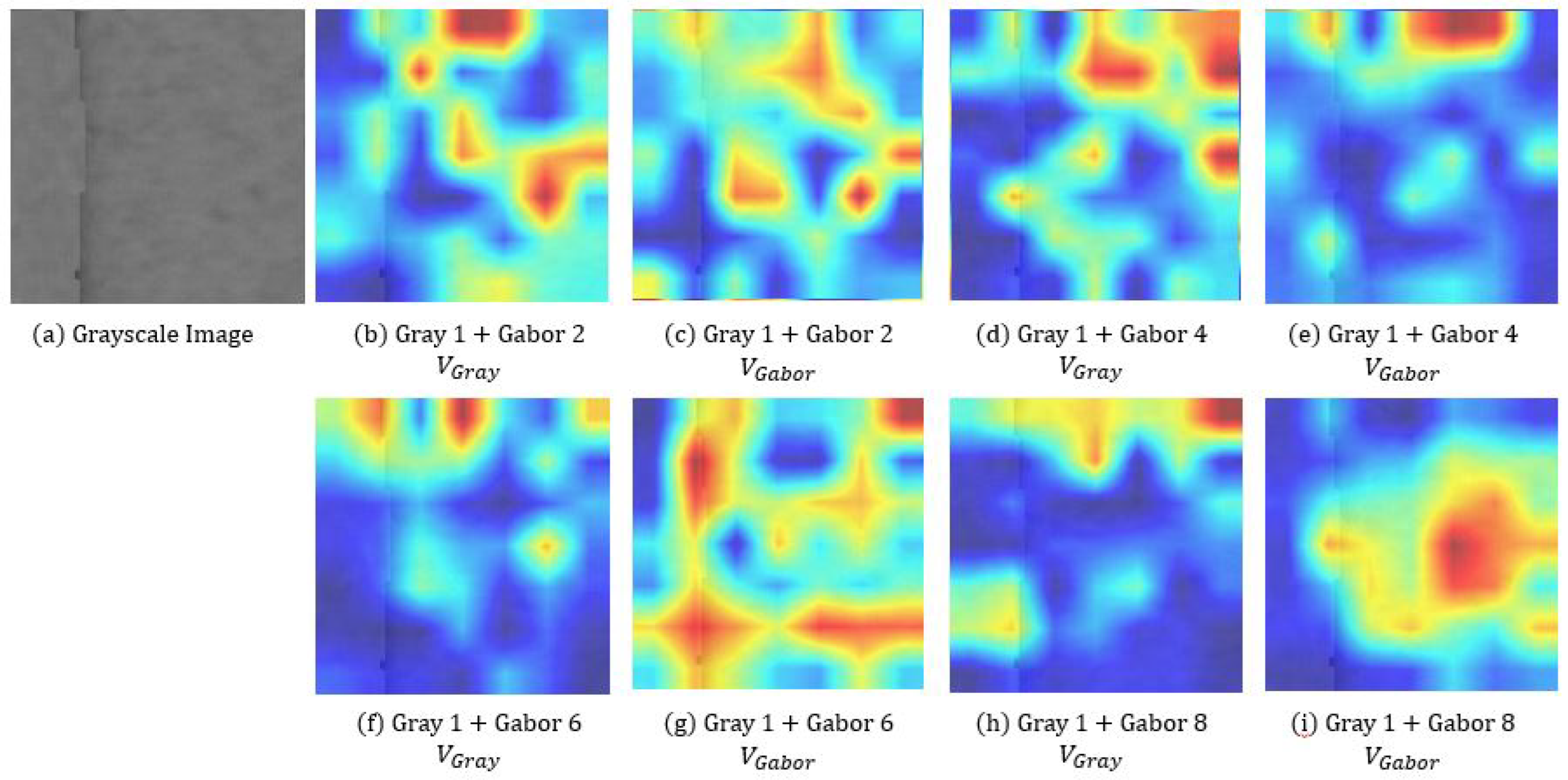
As a result of the experiment, the Gabor filter method was more accurate than the method without using it, and the single-stream structure in the MT dataset and the dual-stream structure in the CCM dataset had higher accuracy. Through this, the performance of single and dual-stream structures can be different depending on the dataset’s characteristics (background, degree of stain). In addition, it was confirmed that selecting N Gabor filter images based on the IDM value is more accurate than using all eight images without selecting them. Through this, it was confirmed that among the Gabor filter images, there are images with important information and other images with lower accuracy due to noise. In addition, it was confirmed that the stream in which the Gabor image was input by outputting the CAM image finds stain.
The disadvantage of the proposed method is that the method for selecting N Gabor filter images depends on the dataset. Although it was confirmed that the method using Gabor filter images is more accurate than the method without, the value of selecting N Gabor filter images according to the dataset must be directly compared with learning and evaluation. It would be nice always to find a good method, but you have to find N chapters while comparing yourself.
Developing a method to calculate optimized Gabor filter parameters for defect classification of datasets through deep learning without using static Gabor filter parameters is planned as a future study. In addition, a study on the structure of a CNN that effectively detects stain defects will be conducted.

Author Contributions

Conceptualization, M.-H.H. and T.-H.P.; methodology, M.-H.H.; software, M.-H.H.; validation, M.-H.H., Y.-G.K. and T.-H.P.; formal analysis, Y.-G.K.; investigation, M.-H.H.; resources, M.-H.H.; data curation, M.-H.H.; writing—original draft preparation, Y.-G.K.; writing—review and editing, Y.-G.K.; visualization, M.-H.H.; supervision, T.-H.P.; project administration, T.-H.P.; funding acquisition, T.-H.P. All authors have read and agreed to the published version of the manuscript.

Funding

This research was supported by the MSIT (Ministry of Science and ICT), Korea, under the Grand Information Technology Research Center support program (IITP-2023-2020-0-01462) supervised by the IITP (Institute for Information & communications Technology Planning & Evaluation). This work was supported by Institute of Information & Communications Technology Planning & Evaluation (IITP) grant funded by the Korea government (MSIT) (No. 2022-0-00795, Development of Moire-Pattern Type 3D Camera System for AI Based Analysis).

Institutional Review Board Statement

Not applicable.

Informed Consent Statement

Not applicable.

Data Availability Statement

Compact Camera Module Dataset is the company’s data. Since it is personal information, it cannot be disclosed.

Conflicts of Interest

The authors declare no conflict of interest.

References

  1. Kong, L.; Shen, J.; Hu, Z.; Pan, K. Detection of water-stains defects in TFT-LCD based on machine vision. In Proceedings of the 2018 11th International Congress on Image and Signal Processing, BioMedical Engineering and Informatics (CISP-BMEI), Beijing, China, 13–15 October 2018. [Google Scholar]
  2. Yang, H.; Song, K.; Mei, S.; Yin, Z. An accurate mura defect vision inspection method using outlier-prejudging-based image background construction and region-gradient-based level set. IEEE Trans. Autom. Sci. Eng. 2018, 15, 1704–1721. [Google Scholar] [CrossRef]
  3. Zhang, Y.J.; Joo, H.; Kim, J.S. Fast detection of Mura defects based on modified watershed algorithm. J. Inst. Control. Robot. Syst. 2017, 23, 446–454. [Google Scholar] [CrossRef]
  4. Wang, X.; Dong, R.; Li, B. TFT-LCD Mura defect detection based on ICA and multi-channels fusion. In Proceedings of the 2016 3rd International Conference on Information Science and Control Engineering (ICISCE), Beijing, China, 8–10 July 2016. [Google Scholar]
  5. Su, C.; Wang, H.; Lin, Q.; Zhao, D.X.; Zhu, J.L. Research on textile stain detection technique based on machine vision. In Proceedings of the 2009 International Symposium on Computer Network and Multimedia Technology, Wuhan, China, 18–20 January 2009. [Google Scholar]
  6. Han, Y.; Shi, P. An adaptive level-selecting wavelet transform for texture defect detection. Image Vis. Comput. 2007, 25, 1239–1248. [Google Scholar] [CrossRef]
  7. Ngo, C.; Park, Y.J.; Jung, J.; Hassan, R.U.; Seok, J. A new algorithm on the automatic TFT-LCD mura defects inspection based on an effective background reconstruction. J. Soc. Inf. Disp. 2017, 25, 737–752. [Google Scholar] [CrossRef]
  8. Bi, X.; Xu, X.; Shen, J. An automatic detection method of Mura defects for liquid crystal display using real Gabor filters. In Proceedings of the 2015 8th International Congress on Image and Signal Processing (CISP), Shenyang, China, 14–16 October 2015. [Google Scholar]
  9. Bi, X.; Zhuang, C.; Ding, H. A new mura defect inspection way for TFT-LCD using level set method. IEEE Signal Process. Lett. 2009, 16, 311–314. [Google Scholar]
  10. Mao, C.; Gururajan, A.; Sari-Sarraf, H.; Hequet, E. Machine vision scheme for stain-release evaluation using Gabor filters with optimized coefficients. Mach. Vis. Appl. 2012, 23, 349–361. [Google Scholar] [CrossRef]
  11. Tsai, D.M.; Lin, C.P. Fast defect detection in textured surfaces using 1D Gabor filters. Int. J. Adv. Manuf. Technol. 2002, 23, 664–675. [Google Scholar] [CrossRef]
  12. Xiao, L.; Huang, T.; Wu, B.; Hu, Y.; Zhou, J. Surface defect detection using hierarchical features. In Proceedings of the 2019 IEEE 15th International Conference on Automation Science and Engineering (CASE), Vancouver, BC, Canada, 22–26 August 2019. [Google Scholar]
  13. Su, T.Y.; Ting, P.J.; Chang, S.W.; Chen, D.Y. Superficial punctate keratitis grading for dry eye screening using deep convolutional neural networks. IEEE Sensors J. 2019, 20, 1672–1678. [Google Scholar] [CrossRef]
  14. Singh, R.B.; Kumar, G.; Sultania, G.; Agashe, S.S.; Sinha, P.R.; Kang, C. Deep learning based MURA defect detection. EAI Endorsed Trans. Cloud Syst. 2019, 5. [Google Scholar] [CrossRef] [Green Version]
  15. Yang, H.; Mei, S.; Song, K.; Tao, B.; Yin, Z. Transfer-learning-based online Mura defect classification. IEEE Trans. Semicond. Manuf. 2017, 31, 116–123. [Google Scholar] [CrossRef]
  16. Wang, R.; Guo, Q.; Lu, S.; Zhang, C. Tire defect detection using fully convolutional network. IEEE Access 2019, 7, 43502–43510. [Google Scholar] [CrossRef]
  17. Almeida, T.; Moutinho, F.; Matos-Carvalho, J.P. Fabric Defect Detection with Deep Learning and False Negative Reduction. IEEE Access 2021, 9, 81936–81945. [Google Scholar] [CrossRef]
  18. Xu, L.; Lv, S.; Deng, Y.; Li, X. A weakly supervised surface defect detection based on convolutional neural network. IEEE Access 2020, 8, 42285–42296. [Google Scholar] [CrossRef]
  19. Wang, S.; Liu, Y.; Qing, Y.; Wang, C.; Lan, T.; Yao, R. Detection of insulator defects with improved ResNeSt and region proposal network. IEEE Access 2020, 8, 184841–184850. [Google Scholar] [CrossRef]
  20. Dong, Y.; Wang, J.; Wang, Z.; Zhang, X.; Gao, Y.; Sui, Q.; Jiang, P. A deep-learning-based multiple defect detection method for tunnel lining damages. IEEE Access 2019, 7, 182643–182657. [Google Scholar] [CrossRef]
  21. Yang, J.; Li, S.; Wang, Z.; Yang, G. Real-time tiny part defect detection system in manufacturing using deep learning. IEEE Access 2019, 7, 89278–89291. [Google Scholar] [CrossRef]
  22. Ouyang, W.; Xu, B.; Hou, J.; Yuan, X. Fabric defect detection using activation layer embedded convolutional neural network. IEEE Access 2019, 7, 70130–70140. [Google Scholar] [CrossRef]
  23. Chen, Y.F.; Yang, F.S.; Su, E.; Ho, C.C. Automatic defect detection system based on deep convolutional neural networks. IEEE Access 2019, 7, 1–4. [Google Scholar] [CrossRef]
  24. Hou, W.; Tao, X.; Xu, D. Combining Prior Knowledge with CNN for Weak Scratch Inspection of Optical Components. IEEE Trans. Instrum. Meas. 2021, 70, 1–11. [Google Scholar] [CrossRef]
  25. He, K.; Zhang, X.; Ren, S.; Sun, J. Deep residual learning for image recognition. In Proceedings of the IEEE Conference on Computer Vision and Pattern Recognition, Las Vegas, NV, USA, 27–30 June 2016. [Google Scholar]
  26. Redmon, J.; Divvala, S.; Girshick, R.; Farhadi, A. You only look once: Unified, real-time object detection. In Proceedings of the IEEE Conference on Computer Vision and Pattern Recognition, Las Vegas, NV, USA, 27–30 June 2016. [Google Scholar]
  27. Tabernik, D.; Šela, S.; Skvarč, J.; Skočaj, D. Segmentation-based deep-learning approach for surface-defect detection. J. Intell. Manuf. 2020, 31, 759–776. [Google Scholar] [CrossRef] [Green Version]
  28. Huang, Y.; Qiu, C.; Yuan, K. Surface defect saliency of magnetic tile. Vis. Comput. 2020, 36, 85–96. [Google Scholar] [CrossRef]
  29. Tao, X.; Zhang, D.; Ma, W.; Liu, X.; Xu, D. Automatic metallic surface defect detection and recognition with convolutional neural networks. Appl. Sci. 2018, 8, 1575. [Google Scholar] [CrossRef] [Green Version]
  30. Rudolph, M.; Wehrbein, T.; Rosenhahn, B.; Wandt, B. Fully convolutional cross-scale-flows for image-based defect detection. In Proceedings of the IEEE/CVF Winter Conference on Applications of Computer Vision, Waikoloa, HI, USA, 3–8 January 2022. [Google Scholar]
  31. Ha, M.-H.; Park, T.-H. Compact Camera Module Cover Defect Classification using Quadtree Decomposition based Deep Learning. J. Inst. Control. Robot. Syst. 2021, 27, 626–632. [Google Scholar] [CrossRef]
  32. Selvaraju, R.R.; Cogswell, M.; Das, A.; Vedantam, R.; Parikh, D.; Batra, D. Grad-cam: Visual explanations from deep networks via gradient-based localization. In Proceedings of the IEEE International Conference on Computer Vision, Venice, Italy, 22–29 October 2017. [Google Scholar]
Figure 1. Stain defect classification system.
Applsci 13 04540 g001
Figure 2. Gabor image according to phase in MT stain image. (a) gray-scale inspection image; from (bi) Gabor filter images according to phase.
Applsci 13 04540 g002
Figure 3. Gabor image according to phase in CCM stain image. (a) gray-scale inspection image; from (bi) Gabor filter images according to phase.
Applsci 13 04540 g003
Figure 4. Single-stream network structure based on ResNet50.
Applsci 13 04540 g004
Figure 5. Dual-stream network structure based on ResNet50.
Applsci 13 04540 g005
Figure 6. Magnetic Tile Dataset (Left: image, Right: Stain Defect segmentation image).
Applsci 13 04540 g006
Figure 7. Compact Camera Module Dataset (Left: image, Right: Stain Defect segmentation image).
Applsci 13 04540 g007
Figure 8. CAM image result for CCM Stain image in a Single-stream Network.
Applsci 13 04540 g008
Figure 9. CAM image result for CCM Stain image in a Dual-stream Network.
Applsci 13 04540 g009
Figure 10. CAM image result for CCM OK image in a Single-stream Network.
Applsci 13 04540 g010
Figure 11. CAM image result for CCM OK image in a Dual-stream Network.
Applsci 13 04540 g011
Table 1. Dual-stream network configuration.
LayerOutput Size I Gray stream s 1 , s 2 , , s N stream
Input224 × 224224 × 224 @ 1224 × 224 @ N
Conv112 × 1127 × 7, 64, stride 27 × 7, 64, stride 2
pooling56 × 563 × 3, stride 23 × 3, stride 2
Res_Block156 × 56 1 × 1 , 64 3 × 3 , 64 1 × 1 , 256 × 3 1 × 1 , 64 3 × 3 , 64 1 × 1 , 256 × 3
Res_Block228 × 28 1 × 1 , 128 3 × 3 , 128 1 × 1 , 512 × 4 1 × 1 , 128 3 × 3 , 128 1 × 1 , 512 × 4
Res_Block314 × 14 1 × 1 , 256 3 × 3 , 256 1 × 1 , 1024 × 6 1 × 1 , 256 3 × 3 , 256 1 × 1 , 1024 × 6
Res_Block47 × 7 1 × 1 , 512 3 × 3 , 512 1 × 1 , 2048 × 3 1 × 1 , 512 3 × 3 , 512 1 × 1 , 2048 × 3
Concat4096 × 1Average pool
Output2 × 1Fully Connected
Table 2. Magnetic tile dataset.
TypeTrainValidationTest
OK19358100
Stain18860100
Total381118200
Table 3. Performance of proposed method on magnetic tile dataset.
Network StructureNumber of Gray ImageNumber of Gabor ImagesPrecisionRecallF1-Score
Single-stream1093.297.695.3
Single-stream0896.799.097.8
Single-stream1896.599.097.7
Dual-stream1895.899.497.6
Table 4. Performance of defect detection method on magnetic tile dataset.
MethodPrecisionRecallF1-Score
SEGDEC75.192.282.0
MCuePush98.696.697.6
CS-FLOW99.690.494.7
Proposed96.799.097.8
Table 5. Compact camera module dataset.
TypeTrainValidationTest
OK35396100
Stain34682100
Total699178200
Table 6. Performance of proposed method on compact camera module dataset.
Network StructureNumber of Gray ImageNumber of Gabor ImagesPrecisionRecallF1-Score
Single-stream1079.693.285.7
Single-stream0896.697.296.8
Single-stream1892.792.292.3
Dual-stream1889.593.091.1
Table 7. Performance of defect detection method on compact camera module dataset.
MethodPrecisionRecallF1-Score
SEGDEC56.210071.9
MCuePush85.491.488.3
CS-FLOW50.010066.7
Proposed96.697.296.8
Table 8. Performance according to the number of gabor images on magnetic tile dataset.
Network StructureNumber of Gray ImageNumber of Gabor ImagesPrecisionRecallF1-Score
Single-stream1295.498.496.9
1498.698.298.4
1696.999.298.0
1896.599.097.7
Dual-stream1296.199.097.6
1495.196.695.8
1695.498.697.0
1895.899.497.6
Table 9. Performance according to the number of gabor images on compact camera module dataset.
Network StructureNumber of Gray ImageNumber of Gabor ImagesPrecisionRecallF1-Score
Single-stream1299.698.499.0
1496.696.896.7
1696.696.296.3
1892.792.292.3
Dual-stream1299.699.099.3
1497.897.697.7
1694.594.294.3
1889.593.091.1
Disclaimer/Publisher’s Note: The statements, opinions and data contained in all publications are solely those of the individual author(s) and contributor(s) and not of MDPI and/or the editor(s). MDPI and/or the editor(s) disclaim responsibility for any injury to people or property resulting from any ideas, methods, instructions or products referred to in the content.

