Evaluation of a Cut Interruption Algorithm for Laser Cutting Steel and Aluminum with a High-Speed Camera

Abstract

We report on a monitoring system based on a high-speed camera for fiber laser fusion cutting. The monitoring system is used without an external illumination retrofit on a conventional cutting head, with the optical path aligned coaxially to the incident laser, permitting a direct, spatially, and temporally resolved detection of the melt pool area in the cut kerf from the top view. The dependence of the melt pool area on laser processing parameters such as laser power and feed rate are thus evaluated for stainless steel, zinc-coated steel, and aluminum, respectively. The signal characteristics of the images captured from the melt pool are examined in the visible spectral range of the emitted secondary thermal radiation from the process zone. An ad hoc developed image processing algorithm analyzes the spectral and geometric information of the melt pool from high-speed camera images and distinguishes between complete and incomplete cuts.

1. Introduction

Fiber laser cutting is an effective and well-established method for processing different types of metals in industry [1,2]. Despite this broad use in industry and comprehensive scientific studies on fiber laser cutting [3], still, a demand exists to provide a reliable monitoring system for in situ quality control, especially for aluminum. In addition to everyday disturbance variables, e.g., unclean optics, thermal lens effects, and variation in material properties, the high fluid dynamics of the melt pool and complex laser material interaction within the kerf challenge the successful monitoring and detection of the cut quality [4]. During laser fusion cutting, the material on the kerf front is kept continuously molten by the focused laser radiation and blown out of the kerf by an inert gas jet [5]. Specifically, the behavior of the melt flow dynamic on the cutting front has a strong influence on the cut quality [6], with a stable, fast, and smooth melt flow being preferable and leading to an overall better cut quality [7].

Common quality losses for laser fusion cutting are the formation of interrupted striation patterns on the kerf wall, adhesion of burr on the bottom edge, and cut interruptions. Striations on the kerf wall are considered to be linked to the boundary layer between gas flow and melt film [8]. Cuts with interrupted striations show higher fluctuations of the cut front and a local increase in the melt film, resulting in an increase in the absorbed irradiance [9]. For higher feed rates, the angle of the kerf increases, resulting in a larger absorbing area irradiated by the laser [10]. Excessively high temperatures in the kerf cause local vaporization, in turn disturbing the melt flow and resulting in a deterioration of the quality with interrupted striation patterns [11] and the formation of burr [12]. Burr forms when parts of the melt adhere to the lower cut edge. The main reason for this is the momentum of the melt flow, which is not sufficient to overcome the adhesion force [13]. Furthermore, with improper parameters, such as low laser power and assisted gas pressure or too high a feed rate and nozzle-to-workpiece distance, cutting interruption may occur [14]. As a result, the workpiece cannot be detached from the sheet panel, hampering automized pick-and-place machines, necessitating rework, or increasing waste. Therefore, the key condition for any quality controlling monitoring system is the capability to spot the process zone spatially and temporally resolved, which necessitates an imaging sensor to observe the whole kerf with a high sampling rate due to the dynamics of the melt. With respect to the increasing demand for resource efficiency, cutting interruptions are undesirable, and autonomously operating cutting machines with quality monitoring are highly demanded.

In contrast to laser welding systems or CO₂ laser-based cutting systems, for which various sensor concepts have already been reported [15,16], quality monitoring setups for laser fusion cutting using fiber lasers, especially for non-steel materials, are comparatively rarely reported or in industrial use, despite the similar or comparable monitoring and sensor concepts. Systems for quality monitoring based on image sensors have been reported for CO₂ laser cutting with external illumination [17] and without external illumination [18,19]. In recordings with external illumination, a band-pass filter or equivalent is used in order to record only the illuminating wavelength for the purpose of imaging the surface and structure of the kerf. In contrast, sensor systems without external illumination record the thermal process radiation from the process zone. Coaxial monitoring approaches for near-infrared laser fusion cutting demonstrate a correlation between the obtained image and the cut quality [20,21]. Whereas for fiber laser flame cutting, coaxial monitoring is more difficult due to the fact that the cutting distortion occurs outside the observation zone, as monitoring is limited by the field of view through the nozzle [22]. To visualize the cutting process inside the kerf, approaches with high-speed cameras positioned off-axial and aligned in the cutting direction are also reported [23,24] also a trim-cut technique through a transparent substrate by a side visual monitoring set up for clear visualization of the melt front inside the kerf [25,26,27], as well as a high-speed x-ray imaging system [9,10] have been demonstrated. These methods provide valuable insights into melt pool dynamics, melt flow velocity, and the geometry of the cutting front and the cutting kerf.

Next to imaging sensors, monitoring systems based on photodiodes have also been developed for quality measurements of laser process [28,29,30] as an alternative to quality monitoring with camera sensors. These are more affordable and favor real-time monitoring, which benefits industrial applications.

In addition to the sensor technology, an evaluation algorithm is likewise essential for quality monitoring, in particular for industrial applications. To detect and predict cut interruption, a cross-correlation algorithm [31] and a polynomial logistic regression model [32] have been reported. Recent reports show neural network approaches for cut quality monitoring [33,34] and to predict the kerf width for remote laser cutting calculated from the laser processing parameters [35].

Against this background, in this article, we present a coaxial in situ high-speed camera setup, which can be integrated and retrofitted into a conventional fiber laser cutting head. In contrast to earlier studies [36], we extend our previous research to observe the melt pool during the laser cutting of zinc-coated steel, stainless steel, and aluminum with a high-speed camera directly from the top view in the visible spectral range on the emitted thermal process radiation, spatially and temporally resolved. Furthermore, we detect complete and incomplete cuts with an algorithm adapted for stainless steel, zinc-coated steel, and aluminum.

2. Materials and Methods

2.1. Laser Cutting Experiments

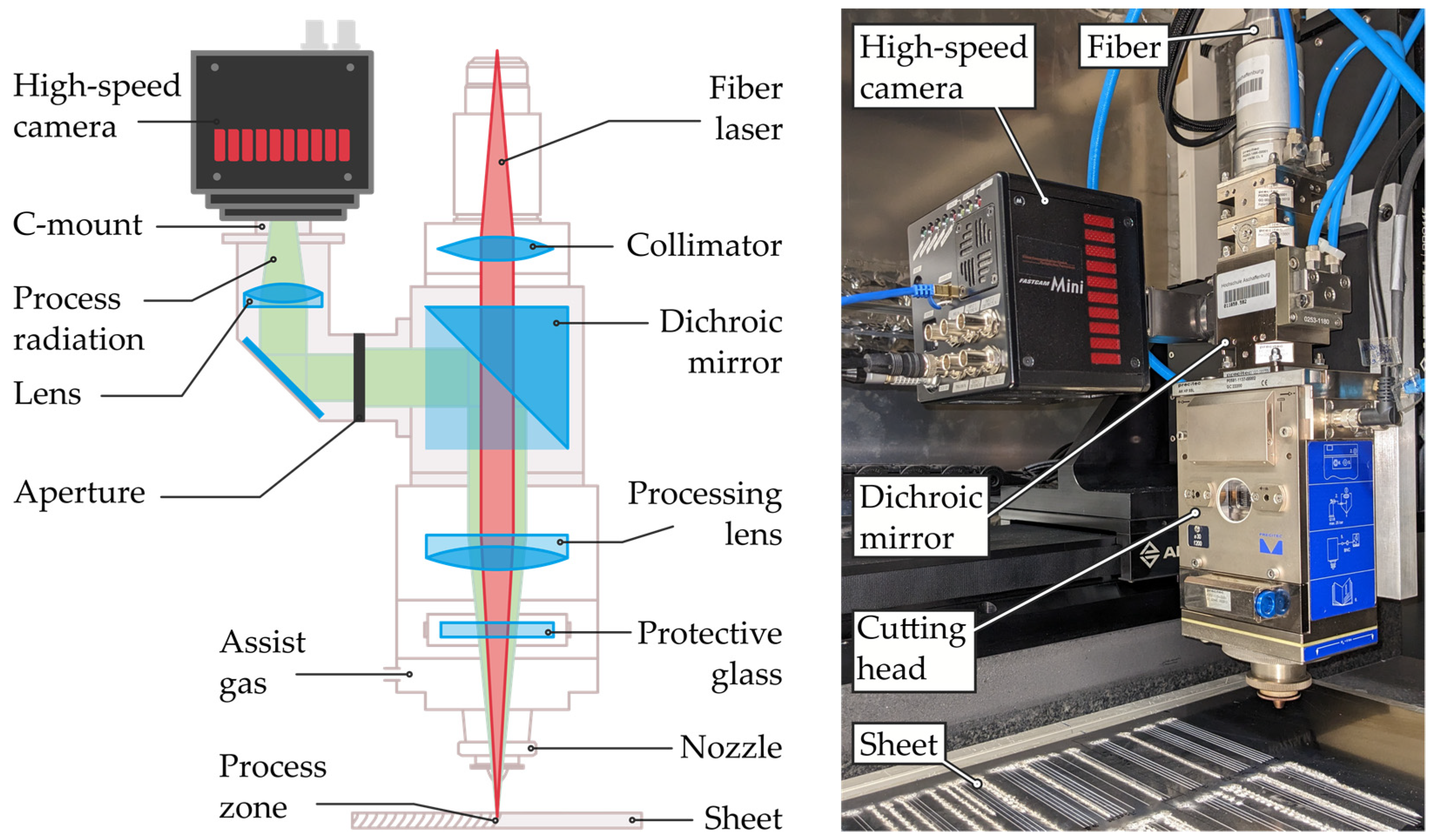
The series of experiments were performed with a 4-kW multimode fiber laser (IPG Photonics, YLS-4000, Burbach, Germany) with an emission wavelength of λ of 1070 nm, a beam quality factor M² of 8.5, a beam parameter product of 2.9 mm×mrad, and a fiber core diameter of 100 µm. The laser beam was collimated and focused by a cutting head (Precitec, HP SSL, Gaggenau, Germany) with a focal length of the collimator lens of 100 mm and a focal length of the processing lens of 200 mm, resulting in a focal diameter of 200 µm. The cutting head was moved by a direct linear drive over the sheet on a conventional 2D flatbed. A nozzle with a diameter of 2.0 mm was mounted, and a stand-off distance of 1.0 mm was adjusted.

Figure 1 shows the applied detection setup, which was intended to be an integrated retrofit between the collimator and processing lens, consisting of a dichroic mirror, an aperture, and a lens for focusing with a focal length of 200 mm for a 1:1 projection to the camera image. The dichroic mirror was designed to reflect the visible spectral components of the thermal process radiation towards the high-speed camera while transmitting the wavelength of the fiber.

The primary laser beam, represented by a red line, was collimated, transmitted through a dichroic mirror, and focused by the process lens onto the sheet. The thermal process radiation from the cutting kerf, represented by a green line, propagates omnidirectionally from the process zone, partly also into the direction of the cutting head through the nozzle, where it was collimated by the processing lens. The reflected radiation was separated optically by a dichroic mirror, whose dielectric coating was transmissive for the emission wavelength of the laser and reflective for the visible thermal radiation from the process zone. The thermal radiation was then guided to the high-speed camera, where it was recorded. The intention of this monitoring setup was to monitor the thermal radiation in the visible spectrum during the cutting process in situ from the perspective of the cutting head.

The cuts were performed in stainless steel with a sheet thickness of 1.5 mm, zinc-coated steel with a sheet thickness of 1.0 and 3.0 mm, and aluminum with a sheet thickness of 1.0, 3.0, and 5.0 mm, respectively. To measure the signal characteristics associated with the melt pool, a complete cut was performed for each material and sheet thickness. Low cut qualities and incomplete cuts were enforced by too-high feed rates and too-low laser power. The laser power varied between 2.0 and 4.0 kW, and the feed rate was between 30 and 300 mm/s. The focus position was set to the bottom of the sheet, and nitrogen was used as the assist gas in all experiments. The variation of the cut parameters to distinguish between complete and incomplete cuts is shown in

Table 1. Variation of the cut parameters.

Material	Sheet Thickness (mm)	Laser Power (kW)	Laser Power Steps (kW)	Feed Rate (mm·s−1)	Feed Rate Steps (mm·s−1)
Stainless steel	1.5	2.0–4.0	0.5	60–220	20
Zinc coated steel	1.0			150–300	25
	3.0			40–100	10
Aluminum	1.0			180–300	20
	3.0			40–160	20
	5.0			30–90	10

.

2.2. Monitoring Setup

The high-speed camera (Photron, Fastcam Mini AX50, Tokyo, Japan) contains a CMOS chip with a square pixel size of 20 × 20 µm² and a relative spectral sensitivity between 400 and 700 nm. The recordings were saved on an onboard ring buffer on the camera and must be downloaded after capturing. The maximum image size depends on the variable sampling rate and decreases for higher sample rates. To visualize the thermal radiation for stainless steel and zinc-coated steel, the kerf is recorded with a frame rate of 20·10³ fps and an image size of 256 × 256 pixels. The exposure time is set to 20 µs to prevent overexposure.

As the melting temperature for aluminum is significantly lower than for steel, the thermal emission intensity decreases considerably for aluminum. In general, the exposure time depends on the sampling rate and cannot be set longer than the inverse of the sampling rate. For too short exposure times (i.e., high sampling rates), the camera cannot accumulate sufficient process radiation from the melt in the kerf. Therefore, to visualize the thermal radiation for cuts in aluminum, the exposure time had to be set to 1.0 ms and the sampling rate to 1·10³ fps accordingly.

The process radiation from the cutting kerf was recorded without additional illumination to measure the thermal radiation solely.

2.3. Evaluation of the Images

To distinguish complete cuts from incomplete cuts during the cutting process, spectral and geometric information from the melt pool in the kerf was evaluated for the image analysis, as shown in Figure 2. Each recorded image I(u,v,c) was a two-dimensional function with the column in the x-direction and rows in the y-direction for each red, green, and blue color channel. However, since the information from the red color channel appears similar to the information from the green color channel, only the green and blue parts were used for further calculations. As common for digital images, the origin is located at the top-left. Consequently, the x-axis is oriented from left to right, whereas the y-axis is oriented from top to bottom. The information about the individual red, green, and blue color channels was correspondingly provided with a data depth of eight bits, i.e., each color channel was provided with 256 gradients. To reduce the amount of data, only the spatial region of interest was used, and the area outside of the nozzle’s field of view was cut out. In the first step of the algorithm, the image was binarized bw(u,v,c) separately for each channel with the threshold t_B = 50. For a lower threshold, a larger area of the melt pool was detected up to the edges of the kerf or the edge of the nozzle’s field of view. At high thresholds, smaller or no amount of melt was detected in the kerf, especially for the blue. This leads to almost identical melt pool sizes for different cutting experiments. It is also worth noting that the threshold value might need to be adjusted depending on the previous image processing steps, process parameters, and camera settings.

$$bw\left(u,v,c\right)=\{\begin{array}{cc}1,\hfill & \hfill if I \left(u,v,c\right)\ge t_B\\ 0,\hfill & \hfill otherwise\end{array}$$

(1)

The binarized image was then used to calculate the features, including the area, ferret diameter, and position of the melt pool. To calculate the area of the melt A_melt, all white pixels of the binarized images were summed.

$$A{\left(c\right)}_{melt}={\displaystyle \sum }_{i=1}^u{\displaystyle \sum }_{j=1}^{v}bw\left(i,j,c\right)$$

(2)

The ferret diameter, in general, describes the distance between two parallel tangents of an object. In our image analysis, it describes the minimum and maximum distance of the melt pool area.

In parallel, the edges of the melt pool were extracted by a canny algorithm in order to subsequently calculate the geometry of an ellipse in the edge of the melt in the direction of the feed rate. For edge detection, the binarized image bw(u,v,c) was initially filtered with a gaussian filter for noise reduction with the filter function H(i,j) and a standard deviation σ of 0.5.

$$b{w}^{\prime }\left(u,v,c\right)\leftarrow {\displaystyle \sum }_{i=-1}^{i=1}{\displaystyle \sum }_{j=-1}^{j=1}bw\left(u+i,v+j,c\right)·H\left(i,j\right)$$

(3)

$$H\left(i,j\right)=e^{-\frac{i^2+j^2}{2{\mathsf{\sigma }}^2}}$$

(4)

Subsequently, for edge detection, a gradient value G was calculated as a directional filter response in the horizontal and vertical directions. Accordingly, all maxima were white, i.e., the edge M and all zero values were black.

$$\nabla G\left(u,v,c\right)=\left(\begin{array}{c}{G}_x\left(u,v,c\right)\\ G_y\left(u,v,c\right)\end{array}\right)=\left(\begin{array}{c}\frac{\partial b{w}^{\prime }}{\partial x}\left(u,v,c\right)\\ \frac{\partial b{w}^{\prime }}{\partial y}\left(u,v,c\right)\end{array}\right)$$

(5)

$$M\left(u,v,c\right)=\sqrt{G_x^2+G_y^2}$$

(6)

The final edge selection M_T(u,v,c) was then performed using a hysteresis thresholding method. In the hysteresis thresholding method, two thresholds, T1 and T2, were used to first search for pixels in the image that are greater than T2. Afterward, the edges adjacent to these pixels that are larger than T1 were marked as edges. Here T1 = 5% and T2 = 9% of the maximum intensity in the image. These threshold value pairs have a large margin at which the edges of the melt pool are detected. Only for very large and small threshold values the detection along the edge can be incorrect, which leads to interruption of the detection along the edge line.

The melt pool width w_melt was calculated from the vertical axis of the ellipse and the length l_melt from the horizontal axis.

$$w_{melt}=\max \left[M_T\left(u\right)\right]-\min \left[M_T\left(u\right)\right]$$

(7)

$$l_{melt}=\max \left[M_T\left(v\right)\right]-\min \left[M_T\left(v\right)\right]$$

(8)

Eventually, the values of the melt pool size, the ferret diameter, the axis of the ellipse, and the position of the melt in the kerf for the green and blue color channels were stored for each individual frame. Finally, a moving average was calculated since individual peaks interfere with the evaluation, with a window width of 300 frames (15 ms) for stainless steel and zinc-coated steel, respectively, with a window width of 15 frames for aluminum, due to the shorter sampling rates for aluminum.

A flowchart describing the image evaluation for the determination of spectral and geometric information from the melt pool is illustrated in Figure 3.

In the following evaluation of complete and incomplete cuts, the thermal emissions from the process zone in the green and blue spectral range from the melt are evaluated. These geometric and spectral components of the melt area are denoted as the green and blue melt pool area, respectively.

3. Results & Discussion

3.1. Comparison between Complete and Incomplete Cuts

Figure 4 shows the signal of the melt pool area, calculated using the above-described image processing step, over time during the cutting of a sample. To visualize the difference between a complete (upper row of diagrams) and an incomplete cut (lower row of diagrams), exemplifying results for such cuts in stainless steel and zinc-coated steel are presented. A cut is classified as incomplete if the bottom edge of the kerf resolidifies. This is the case when the laser power is insufficient to penetrate the material or when the melt cannot be driven out of the kerf and adhering burr seals the bottom of the kerf. In addition to the diagrams, for each case, exemplarily chosen frames recorded by the high-speed camera are shown. The timeline of each recording starts after the piercing of the laser. During the time frame, the drives start to accelerate, which leads to the laser cut and is indicated by an increase in the green and blue melt pool areas. Towards the end of the cut, the feed rate decelerates, and a decrease in the melt pool area is visible.

A comparison for incomplete cuts (lower row of Figure 4) reveals remarkable differences in the recorded frames and both the spectral and geometrical information calculated from the melt pool area. During a complete cut, the material is kept molten by the laser and driven out of the kerf by the assist gas pressure. The hottest area of the melt pool, located directly at the cut front, emits more intensely in the blue spectral region and can therefore be seen brighter or white in the recorded image. The cooler regions of the melt, such as the ejected melt further from the cut front, emit less in the blue spectral region and appear darker and more pronounced in the green color channel. In contrast, during an incomplete cut, the melt from the cut front is not completely expelled from the kerf and is partially resolidified in the kerf. In general, an increased melt pool area is observed whenever an incomplete cut is forced by a reduction in laser power or an increase in feed rate.

Moreover, for incomplete and complete cuts, different behaviors in the calculated geometries from the melt pool are observed. As described above, the width of the kerf represents the vertical axis and the length of the horizontal axis of the melt pool. Considering complete cuts, the melt pool appears more circular, with the vertical axis (width) and the horizontal axis (length) of the calculated geometries being almost equal. Incomplete cuts result in a significant change in the melt pool geometry. The not expelled portion of the melt resolidified in the cutting kerf, contributing to the thermal radiation and resulting in a pronounced increase in the horizontal axis of the melt pool length in the route of the feed rate. As, in contrast, the kerf width increases less, the melt pool area appears in an elliptical shape.

In addition, a tendency can be observed that for complete cuts, the signal of the green melt pool area slightly exceeds the signal of the blue melt pool area. For incomplete cuts, the signal of the blue melt pool area converges with the signal of the green melt pool area or exceeds it. This can be assigned to an enhanced temperature when closing the kerf due to the increased irradiated area of the laser, and more thermal radiation is directed toward the cutting head, which can lead to overexposure.

The recorded frames and calculated melt pool areas for aluminum show significant deviations from stainless steel and zinc-coated steel, as depicted in Figure 5. First of all, for complete cuts, significantly lower process radiation is observed, in particular for cutting 1 mm aluminum, despite the longer exposure time. Aluminum, with a melting point of about 933 K, emits almost no radiation in the range of the detectable camera between 400 and 700 nm, especially for the green and blue channels of the camera. The maximum wavelength of the specific spectral radiation at the melting point of aluminum is 3105.9 nm, i.e., in the infrared range. According to Wien’s displacement law, the intensity maximum wavelength shifts to a shorter wavelength at higher temperatures. At an evaporation temperature of about 2743 K for aluminum, the maximum wavelength thus shifts to 1056.4 nm. However, the melt in the kerf emits thermal radiation over a wide spectral region. The spectral distribution depends on the temperature according to Planck’s law, and therefore emissions from the process zone for aluminum can still be recorded, even if the maximum wavelength of the emission for aluminum melt is not directly in the detectable range of the high-speed camera.

Figure 6 shows exemplifying images of the melt pool area in aluminum for 1, 3, and 5 mm. A smoother melt flow can be related to the lower viscosity and surface tension of aluminum at higher temperatures compared to steel [37,38,39]. Higher feed rates or sheet thicknesses result in an increased cut kerf angle. Due to the increased primary laser irradiation area, the melt film increases for aluminum, and also, the local temperature in the kerf rises, which leads to vaporization. A higher emission of the vaporization compared to the melt explains the high blue component and the overexposed white areas in the signal curve for complete cuts and especially for incomplete cuts in aluminum. The actual cooler cut front for aluminum is not assumed to be at the front of the detectable melt pool area, as for steel, but further in the direction of the feed rate, i.e., further to the right from the top view. This occurs because, presumably due to the lower viscosity and surface tension, the melt is removed more quickly from the cut kerf front.

Nevertheless, geometric and spectral information can be calculated from the recorded images, as the resulting vapor plume also reveals similar signal characteristics. In aluminum, it is also observed that for incomplete cuts, the length of the melt pool area increases compared to complete cuts, and the melt pool area appears more elliptical. The melt pool area of the horizontal axis even extends beyond the field of view of the nozzle.

Especially good visible for aluminum is the resulting plasma plume for incomplete cuts, which emerges upwards from the kerf. This plasma plume emits in the UV spectral range, as shown in Figure 5d–f. During an incomplete cut, a white area is visible in the region of the kerf, presumably due to overexposure caused by the longer exposure time due to the shorter sampling rate for aluminum and the addition of the color channels. However, the blue spectral region of the emitting plasma plume is, in addition, clearly visible outside of the kerf in Figure 5d–f. Please note, in cuts for aluminum, a sharp peak can often be detected at the start of each cut, here always at 1.5 s, which is not considered for the measured signal for later observations.

3.2. Dependence on Laser Power and Feed Rate

Figure 7 summarizes the variation of the melt pool area, determined from the high-speed camera top views, versus laser power and feed rate for 1.5 mm stainless steel, 1.0 mm, and 3.0 mm zinc-coated steel, respectively. In general, the melt pool area increases with increasing laser power and feed rate for all sheet thicknesses. Figure 7 shows that the recorded melt pool area is proportional to the laser power at a constant feed rate for a fixed sheet thickness with the investigated process window. During cutting, the absorbed laser power depends not only on the wavelength, polarization, and specific material properties but also on the angle of the kerf, i.e., the effective contact area of the impinging laser radiation. At low feed rates, a small melt pool area is observed, which can be attributed to the fact that in this regime, only a small portion of the laser radiation irradiates the nearly vertical cut front. At higher feed rates, the angle of the kerf becomes flatter, which leads to an enlarged contact area in the cutting direction. The raised flank of the kerf increases the absorption of the laser radiation, which leads to a larger measured intensity of the process radiation by the high-speed camera.

Figure 8 summarizes the variation of the melt pool area in the cut kerf, detected from the high-speed camera top view, as a function of laser power and feed rate for 1.0, 3.0, and 5.0 mm aluminum. In addition, for aluminum, it can generally be seen that the melt pool area increases with increasing laser power and feed rate for all sheet thicknesses. The feed rate, however, does not seem to be directly related to the melt pool area.

If the cutting parameters are unsuitable, e.g., if the feed rate is too high or the laser power too low, incomplete cuts occur, resulting in a significant increase in the melt pool area. Figure 9 compares the distribution of all melt pool areas for complete and incomplete cuts in stainless steel and zinc-coated steel. From this comparison, it can be seen that the melt pool area is not sufficient to distinguish incomplete cuts from complete cuts. Although for most cuts, the size of the melt pool area during an incomplete cut is significantly larger than during a complete cut. It can be observed that the same melt pool area is detected for incomplete and complete cuts in stainless steel and zinc-coated steel. Thus, further characteristics must be used for unambiguous cut interruption detection. The comparison of the melt pool area for complete and incomplete cuts in aluminum is depicted in Figure 10. For cutting aluminum, due to the lower melting temperature and resulting higher sampling rate, incomplete cuts often lead to overexposure of the camera image. This is particularly evident for cuts in a 5 mm aluminum sheet.

3.3. Detection of Incomplete Cuts

To sense and discriminate complete and incomplete cuts, we developed and evaluated an algorithm based on the observation and interpretation of the geometric parameters and properties in the blue and green melt pool areas.

A flowchart specifying the algorithm is shown in Figure 11. As an initial step, the image processing step is performed as described above (cf. Section 2.3) to obtain the area, length, width, ferret diameter, and the center position of the melt pool for the green and blue color channels, respectively. The algorithm for detection of a cutting error was first tested with different thresholds on eight cutting samples, four complete and four incomplete cuts each, for stainless steel, zinc-coated steel, and aluminum, and then applied to all cutting samples. The threshold value for the detection depends on the exposure time, the binarization method of the image processing as well as on the material of the sheet and must also be adjusted for stainless steel, zinc-coated steel, and aluminum.

In the first selection, the blue melt pool area is checked if it is larger than a selected threshold value, which is based on the previously described experimental results and set according to the maximum detection limit. The upper threshold TH1 and lower threshold TH2 are used as preselection to sort out unambiguous incomplete and complete cuts for which incorrect geometries are calculated. This applies to the upper threshold, e.g., for plasma formation, where the images are heavily overexposed for the green and blue color channel, and also for the case where the area for incomplete cuts is significantly larger and extends beyond the field of view of the nozzle. In these cases, a cut is considered incomplete. For complete cuts with low feed rates, where the material is molten only at the laser cut front and immediately expelled out of the kerf, where consequently low process radiation is emitted, the camera is less exposed, and the geometries cannot always be calculated from the melt pool area. In these cases, a complete cut always occurs. Specifically, for the stainless steel, we selected a threshold greater than TH1 = 1600 pixels or less than TH2 = 500 pixels for the preselection of complete and incomplete cuts. For zinc-coated steel, the threshold value for TH1 changes to 900 and TH2 to 450 pixels. These specific threshold values are determined from the comparison of the melt pool areas shown in Figure 8.

The second selection is to check whether the blue melt pool area equals or exceeds the green melt pool area with a threshold value of TH3 = 90% for stainless steel and 95% for zinc-coated steel. In the third selection, it is then checked whether the ellipse enlarges in the direction of the fed rate and meanwhile, the blue melt pool area of the horizontal axis, the vertical axis of the ellipse, or the minimum or maximum ferret diameter passes TH4 and TH5 of 98% of the green melt pool area for stainless steel, respectively TH4 and TH5 of 100% for zinc coated steel. This is the case when the melt collects in the whole kerf and cannot be driven downward and out or expelled upward because the bottom edge of the sheet remains united. Finally, in the fourth selection, it is controlled if the center of the blue and green melt pool area is in the center of the nozzle or the direction of the feed rate since the center point also shifts when the ellipse is enlarged in the feed rate direction.

For aluminum, solely the first selection of the algorithm is applied to distinguish a complete cut from an incomplete cut. The blue melt pool area is checked if it is larger than the threshold TH1 = 2000 pixels. This threshold is determined from the comparison of the melt pool areas for aluminum shown in Figure 9 and refers to the overexposure of the high-speed camera image, where an incomplete cut always occurs for aluminum.

Figure 12 shows the detected signals using the example of complete and incomplete cuts for stainless steel, galvanized steel, and aluminum. It is shown that the selection of one, two, and four occurs in the example of an incomplete cut in 3 mm zinc-coated steel. This indicates that the area of the melt is particularly large, the blue portion exceeds the green portion, and the center of the melt shifts significantly. In the case of an incomplete cut in 1 mm zinc-coated steel, selection three occurs, i.e., the melt pool area is neither too large nor is the blue portion larger than the green portion. However, the melt has an elliptical shape, and the blue melt pool area approaches the width and length of the green melt pool area. In the example of the incomplete cut in stainless steel, a combination of all four selections occurs. For aluminum, as described, only selection one is used to detect incomplete cuts. The example for a complete cut in 3 mm galvanized steel shows an incorrect detection. As can be seen, selection two is triggered occasionally during the cut.

The algorithm described here provides the best detection probability. We have evaluated this algorithm for 220 cutting tests in stainless steel with a sheet thickness of 1.5 mm, zinc-coated steel with a sheet thickness of 1.0 and 3.0 mm, and aluminum with a sheet thickness of 1.0, 3.0, and 5.0 mm. We varied the laser power between 2.0 and 4.0 kW and the feed rate between 30 and 300 mm/s to enforce incomplete cuts. From this series of tests, all 74 incomplete cuts are reliably detected. For five complete cuts out of a total of 146, however, an incomplete cut was detected by the algorithm, which leads to an error of 2.3% for this test series, showing a detection probability that is comparable to other quality monitoring systems for laser cutting [40,41].

4. Conclusions

A monitoring system based on a high-speed camera and an algorithm to distinguish between complete and incomplete cuts during fiber laser fusion cutting of stainless steel with a sheet thickness of 1.5 mm, zinc-coated steel with a sheet thickness of 1.0 and 3.0 mm and aluminum with a sheet thickness of 1.0, 3.0, and 5.0 mm was demonstrated. The thermal radiation was recorded in the visible spectral range without external illumination with a high-speed camera, whereby the cut kerf can be observed coaxially and in situ. For stainless steel, zinc-coated steel, and aluminum, the dependence of thermal radiation on laser power and feed rate was examined. In addition, incomplete cuts caused by too low laser power or too high a feed rate could be detected with our algorithm with an error rate of 2.3% from the signal characteristic of the melt pool.