Abstract
The multi-objective optimization problem is difficult to solve with conventional optimization methods and algorithms because there are conflicts among several optimization objectives and functions. Through the efforts of researchers and experts from different fields for the last 30 years, the research and application of multi-objective evolutionary algorithms (MOEA) have made excellent progress in solving such problems. MOEA has become one of the primary used methods and technologies in the realm of multi-objective optimization. It is also a hotspot in the evolutionary computation research community. This survey provides a comprehensive investigation of MOEA algorithms that have emerged in recent decades and summarizes and classifies the classical MOEAs by evolutionary mechanism from the viewpoint of the search strategy. This paper divides them into three categories considering the search strategy of MOEA, i.e., decomposition-based MOEA algorithms, dominant relation-based MOEA algorithms, and evaluation index-based MOEA algorithms. This paper selects the relevant representative algorithms for a detailed summary and analysis. As a prospective research direction, we propose to combine the chaotic evolution algorithm with these representative search strategies for improving the search capability of multi-objective optimization algorithms. The capability of the new multi-objective evolutionary algorithm has been discussed, which further proposes the future research direction of MOEA. It also lays a foundation for the application and development of MOEA with these prospective works in the future.
1. Introduction
As one of the heuristic search optimization algorithms using population, the evolutionary computation algorithm is easy to apply and implement. It does not require highly deterministic mathematical properties for both problems to be solved and the algorithms to solve these. Its application field has expanded steadily up to this point, attracting the interest of several academics and engineers [1]. Evolutionary multi-objective optimization (EMO) has been used successfully in the field of multi-objective optimization problems, and it has developed into a rather popular field of study [2]. EMO has gained widespread attention and adoption in the scope of evolutionary computation research.
Optimization problems are a common type of problem encountered in engineering applications and scientific research. These problems involve finding the optimal solution or solutions to a particular problem [3]. The problems of single-objective optimization have a single-objective function, while multi-objective optimization problems (MOP) involve multiple-objective functions, and attempt to satisfy all objective functions simultaneously. One solution may be enough for one objective, but it may not perform well on all objectives at the same time. Therefore, there will be a set of compromise solutions, which is called the Pareto optimal set in multi-objective optimization problems [4].
Conventionally, by giving weights to the various objectives, the MOP was often converted into single-objective problems. These single-objective problems can be solved using mathematical programming techniques, which can only obtain the optimal solution under the condition of one weight at one time. The conventional mathematical programming approaches are frequently ineffective and more susceptible to the weight value or the order provided by the objective because the objective function and constraint function of the MOP may have discontinuous, nonlinear, or non-differentiable characteristics. The population of potential solutions is preserved from generation to generation by an evolutionary computation algorithm to achieve the global optimum. By using this population-to-population strategy, it is possible to find the Pareto optimal solutions set for the multi-objective optimization problem. Schaffer introduced the vector evaluation genetic algorithm (VEGA) at the beginning of 1985 [4], which is recognized as the evolutionary computation algorithm’s groundbreaking contribution to resolving the MOP. The non-dominated sorting genetic algorithm (NSGA) was presented by Srinivas and Deb [5], and the multi-objective genetic algorithm (MOGA) was suggested by Fonseca and Fleming [6] The niched Pareto genetic algorithm (NPGA) was propounded by Horn et al. [7]. These algorithms are the pioneer works for MOEA in the evolutionary computation community.
The original evolutionary multi-objective optimization algorithm is the ordinary name for these algorithms. Individual selection using the Pareto level and population diversity maintenance using the fitness-sharing mechanism are features of the primitive generation of evolutionary multi-objective optimization algorithms [8].The second-generation evolutionary multi-objective optimization algorithm, which features an elite retention mechanism, was sequentially proposed from 1998 to 2002. In 1998, the strength Pareto evolutionary algorithm (SPEA) was first proposed by Zitzler and Thiele [9], and SPEA-SPEA2 was improved upon three years later [10]. The Pareto archived evolution strategy (PAES) was proposed by Knowles and Corne in 2000 [11]; shortly after, they proposed enhanced versions of the algorithm, the Pareto binary-based selection algorithm (PESA) [12] and PESA-II [13]. An enhanced version of NPGA, NPGA2, was proposed by Erickson et al. in 2001 [14]. A micro-genetic algorithm (MICRO-GA) was propounded by Coello and Pulido [15]. In 2002, Deb et al. suggested a highly conventional algorithm by enhancing NSGA, i.e., NSGA-II [16].
Since 2003, an EMO algorithm has been developing continuously, and study in the frontier area of evolutionary multi-objective optimization has taken on new characteristics. Several novel algorithm frameworks have been developed as a result of the introduction of certain new evolutionary mechanisms to the discipline of evolutionary multi-objective optimization to more efficiently handle the high-dimensional multi-objective optimization issue [17]. For instance, the multi-objective particle swarm optimization (MOPSO) was suggested by Coello and Lechuga using particle swarm optimization [18], and the non-dominated neighbor immune algorithm (NNIA) was propounded by Gong et al. using the immune algorithm [19] The multi-objective evolutionary algorithm using decomposition (MOEA/D), which merges evolutionary algorithms with classical mathematical programming techniques, was presented by Zhang and Li [20].
Any new technology arises and develops from its application, otherwise, the new technology would be lifeless. To solve the problem of multiclass pattern discrimination in machine learning, Schaffer designed and implemented LS2 based on LS1 using the vector evaluation genetic algorithm in 1985 [4]. Since 1990, MOEA has been widely used in various industries, such as environmental and resource allocation, electrical and electronic engineering, communication and networking, robotics, aerospace, municipal construction, transportation, mechanical design and manufacturing, management engineering, finance, and other scientific research. As the use of MOEA becomes more widespread, its classification and applicability to engineering problems become increasingly important [21]. Nowadays, research on the application of MOEA is one of the most popular topics in the research community. About 50% of the papers focus on solving real-world application problems, which is one of the major research areas for the vitality of MOEA [22]. Some examples include multiobjective optimal control for the wastewater treatment process [23], data mining [24,25], mechanical design [26], mobile network planning [27], portfolio management [28], design of central neural motion controllers for humanoid robots [29], optimal design of perimeter rocket engines [30], QoS routing [31], logistics distribution [32,33], logic circuit design [34], multi-sensor multi-objective tracking data association [35], underwater robot motion planning [36], shop floor scheduling problems [37], design problems for urban water management systems [38], and communication and network optimization [39,40]. The objective of studying MOEA is to apply MOEA to better solve practical problems. Therefore, research on the application of MOEA in various fields is most valuable and meaningful.
Within the growing body of research on this field all over the world, many scholars are writing summaries of the field of evolutionary computation algorithms. In recent years, the rapid development of evolutionary multi-objective optimization has warranted a comprehensive survey of this field, as well as analysis and summary [41]. Many other surveys or reviews in the literature are very novel and worth learning from. These have been organized and categorized into Table 1 for better analysis.

Table 1.
The surveys in the references can be broadly divided into four categories and find the differences between them.
These surveys can be broadly classified into four categories. The first one is a specialized classification of algorithms that use specific techniques. The second one is a classification of algorithms differently based on certain characteristics. The third one is a survey of algorithms for the problem to be solved. The fourth is a survey of algorithms developed according to time. Our survey can be classified as falling into the second category because we classify representative MOEAs from different MOEA search strategies. However, there is still some difference between them, and while classifying the algorithms, we are also investigating the search strategy as a research direction.
This survey primarily selects some representative multi-objective optimization algorithms in view of search strategies in MOEA. This can be considered one of the original aspects of this current work. Their types are many and complex, so it is especially necessary to classify them accordingly to summarize this research field. After analysis and classification, the chaotic evolution can be designed. This is achieved by combining different types of search strategies of multi-objective optimization algorithms to enrich this research area as one of the promising research subjects. Currently, the main reason why the MOEA algorithm is so popular is that it has a wide range of application areas and application prospects. In real-world industry applications, problems often require optimizing many objectives simultaneously, which are complex and nonlinear. Conventional methods may struggle to effectively solve such problems [51]. MOEA is well-suited for tackling these types of problems. In this work, we select and classify representative MOEA, especially search strategies.
The remaining parts of the paper are structured as follows. A brief background on multi-objective evolutionary algorithms is given in Section 2. Section 3 gives a systematic classification and detailed introduction of current evolutionary multi-objective optimization algorithms and their search strategies. In Section 4, evaluation metrics of MOEA are introduced. Section 5 and Section 6 summarize the whole paper and put forward our views on the further development of evolutionary multi-objective optimization.
2. An Overview on Multi-Objective Optimization and Multi-Objective Evolutionary Computation
The multi-objective optimization problem is a pervasive challenge in many areas of practice. It may not be possible to fully achieve all objectives, so each objective must be assigned a relative weight in a scoring method [52]. Determining these weights is a primary issue in this research. Meanwhile, the genetic algorithm inspired by the principles of biological evolution has also gained significant attention [53]. Combining these two approaches allows the global search capabilities of the genetic algorithm to be exploited while avoiding the risk of conventional multi-objective optimization methods becoming stuck in local optima and maintaining population solution diversity. As a result, a genetic algorithm-based multi-objective optimization strategy has been applied across various fields.
The MOP is usually transformed into single-objective problems by weighting and pre-processing, after which they can be solved by mathematical programming methods [47]. However, this method can only yield one optimal solution for a single set of weights per return. Additionally, there is a probability that the objective and constraint functions of problems are discontinuous and nonlinear and cannot be solved by conventional mathematical programming methods. Conventional mathematical programming is ineffective and susceptible to the weights or rankings provided by the objective [54]. A multi-objective optimization solution is often composed through a series of equilibrium solutions, i.e., a collection of optimal solutions organized into many sets of Pareto optimal solutions, with each component being referred to as a Pareto optimal solution [55]. It aims to simultaneously achieve several objectives in each region as efficiently as possible. In multi-objective optimization, since multiple sub-objectives are optimized simultaneously, and these sub-objectives are often in conflict with each other, over-optimization of one sub-objective will inevitably lead to less favorable optimization results for at least one of the other sub-objectives. When dealing with the MOP, we do not try to find the single best solution [43]. In the multi-objective optimization algorithm, there are different optimization objectives for different sub-objective functions. Generally, there are three cases, as follows:
- Minimize all sub-objective functions.
- Maximize all sub-objective functions.
- Minimize the sub-objective function and maximize other sub-objective functions.
2.1. Multi-Objective Problem
A MOP can be formulated as follows in Equation (1).
In Equation (1), is a decision space or a parameter space, is composed of m objective functions, and is called the objective space. However, as most objectives tend to conflict with each other, it is not possible to maximize all objectives simultaneously at any point in . Consequently, a balance was sought between these conflicting objectives.
As opposed to single-objective optimization problems, which typically have a single optimal solution that can be found using standard deterministic mathematical methods, MOP involves multiple competing objectives [45]. In these types of problems, finding a single solution that optimizes all objectives at the same time is difficult because improving the performance of one objective may come at the cost of decreasing the performance of another. In contrast, the solution to a MOP is typically a Pareto solution set, which represents weighing up conflicting objectives [56].
When there are multiple Pareto optimal solutions, it can be challenging to determine which solution is more desirable without additional details. As a result, all Pareto optimal solutions can be considered equally valid. Consequently, finding the most Pareto optimum solutions to a given optimization problem is the primary subject of multi-objective optimization [48]. To achieve this, multi-objective optimization typically focuses on the following two tasks.
- Identify a set of solutions that are as near in terms of probability to the Pareto optimal domain.
- Identify a set of solutions that are as diverse as possible.
The first task must be completed in any optimization task, and a convergence that is not close to one of the real Pareto optimal solution sets is undesirable. Only when a group of solutions has convergence that is close to the real Pareto optimal solution is the set of solutions guaranteed to approach the optimal property [57].
In addition to converging to the approximate Pareto optimal region, the solutions obtained through multi-objective optimization should also be uniformly and sparsely distributed within that region. A good set of solutions for multiple objectives is represented by a diverse set of solutions. In an MOEA, diversity can be defined in both the decision variable space and the objective space [58]. For example, if the Euclidean distance between two solutions is large in the decision variable space, they are considered different in that space. Similarly, solutions that are far apart in the objective space are considered to be diverse. However, for complex and nonlinear optimization problems, good diversity in one space does not necessarily translate to good diversity in the other space. A set of solutions with good diversity must be identified in the relevant space [49].
2.2. Multi-Objective Evolutionary Computation Algorithm
There are many types of multi-objective evolutionary computation algorithms. They can be classified according to certain characteristics. In the existing research, the algorithms based on differential evolution are reviewed, and the method of classification is proposed [42]. In our paper, from the view of different MOEA search strategies, we can classify them as follows:
- Decomposition-based MOEA algorithms.
- Dominant relationship-based MOEA algorithms.
- Evaluation index-based MOEA algorithms.
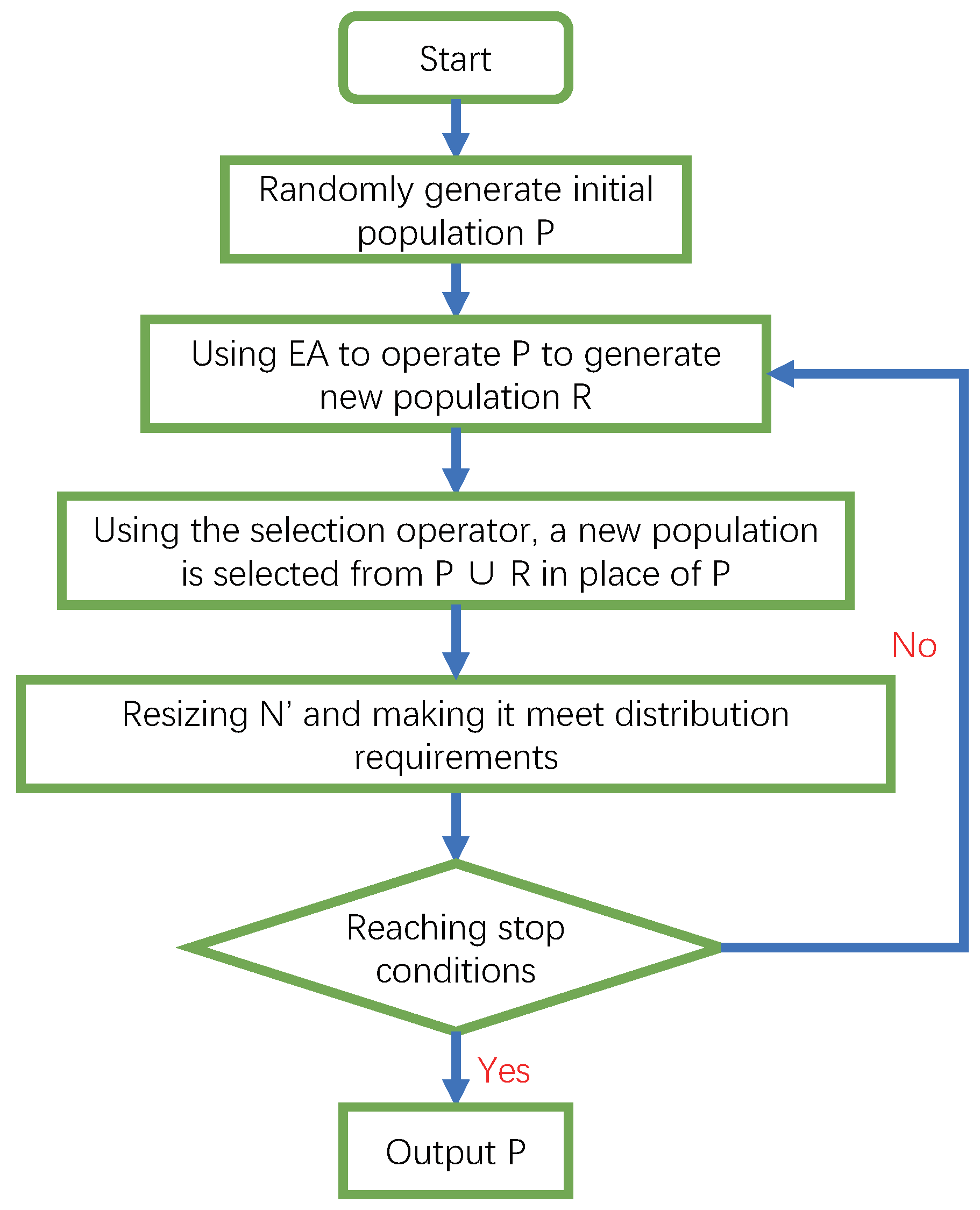
To obtain a deeper understanding of the MOEA search process, we present the basic flow of Pareto-based MOEA, as shown in Figure 1. First, population P is initialized, and an evolutionary computation algorithm, such as a decomposition-based multi-objective evolutionary algorithm, is selected to perform evolutionary operations on P to obtain the new population R. Second, the optimal solution set of is constructed, and the size of the optimal solution set is set to N. If the size of the current optimal solution set N is inconsistent with the size of N, the size of N needs adjustment, and the adjusted N needs to meet the requirements of distribution. It determines whether the algorithm termination conditions have been met. The individuals in N will be copied to the population P to continue in the next round of evolution, otherwise, it will stop. The iteration count of the algorithm is generally used to control its execution.
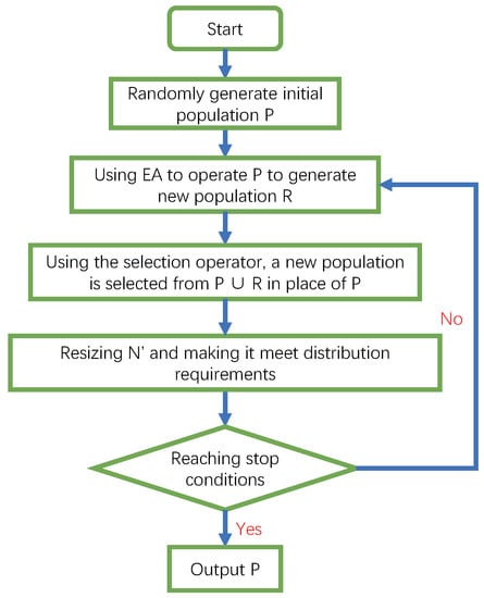
Figure 1.
The basic flow of Pareto-based MOEA. The optimal set of solutions from the previous generation is retained and added to the new generation so that it continues to converge to the true Pareto front. This figure is adopted from [6].
In MOEA, maintaining and incorporating the optimal solution set from the preceding generation into the evolution process of the current generation is a critical requirement for convergence [59]. This allows the evolutionary population’s optimal solution set to converge to the real Pareto front, ultimately leading to a satisfactory evolutionary outcome.
2.3. Multi-Objective Chaotic Evolution Algorithm
2.3.1. Chaos and Chaotic Systems
Chaos means disorder. A simple deterministic system can not only produce simple deterministic behavior but also produce seemingly random uncertain behavior, namely chaotic behavior [60]. Chaos refers to the uncertain or unpredictable random phenomena presented by certain macroscopic nonlinear systems under certain conditions. It is the phenomenon of the integration of certainty and uncertainty, regularity and non-regularity, or orderliness and disorder. At present, there are different ways of understanding and expressing chaos in different disciplines, which reflect the characteristics of its application in their respective fields. Chaos is an aperiodic behavior of a nonlinear dynamic system that is generated within a certain control parameter and has a keen reliance on preliminary conditions. The system in this behavior state is called a chaotic system. Among these, non-linearity is the most fundamental condition for the chaotic behavior of a dynamic system and an inevitable factor for the system. There are four common chaotic systems, namely, a logistic map [61], Hénon map [62], tent map [63], and Gauss map [64].
2.3.2. Multi-Objective Chaotic Evolution Algorithm
EMO algorithms can effectively solve the MOP. The effectiveness of EMO’s optimization process depends on the search algorithm’s capacity to optimize results in addition to Pareto dominance and solution diversity [65]. By including chaotic evolution in the EMO algorithm, reference [66] proposed the multi-objective chaotic evolution algorithm (MOCE) with a powerful search capability. The MOCE algorithm combines the non-dominated sorting and crowding distance methods with the search capacity of the traditional CE algorithm. It does not only aim to maintain the number of Pareto solutions but also strives to maintain their diversity.
2.4. Primary Challenges of Multi-Objective Optimization Study
Due to the close correlation between MOP and practical applications, MOP has become the subject of many research topics.
- Most existing algorithms for solving MOP depend on evolutionary computation algorithms, and a new algorithm framework with a powerful search capability needs to be proposed urgently [67].
- An assessment technique that can objectively reflect the algorithm’s benefits and drawbacks, as well as a collection of test cases, is necessary for the evaluation of a multi-objective optimization algorithm. One of the most significant aspects of the research is the choice and design of assessment techniques and test cases.
- Existing multi-objective optimization algorithms have strengths and weaknesses. An algorithm is effective for solving one problem but may be ineffective for solving other problems. Therefore, how to make the advantages and disadvantages of each algorithm complementary is still a problem to be studied [68].
3. Classification of Multi-Objective Evolutionary Algorithms from the View of Search Strategy
3.1. Decomposition-Based MOEA Algorithms
3.1.1. Weighted Summation Approach
The weighted sum approach is a commonly used linear multi-objective aggregation method [69]. Assuming that the multi-objective problem to be optimized has m total objectives, the function converts MOP into a single objective sub-vector by weighting each objective with a non-negative weight vector = (, ,..., ). The mathematical expression is as shown in Equation (2).
The vector = (, ,..., ) is a set of weight vectors. Each weight component corresponds to the i-th target vector, respectively, for ≥ 0 and the sum of is 1.
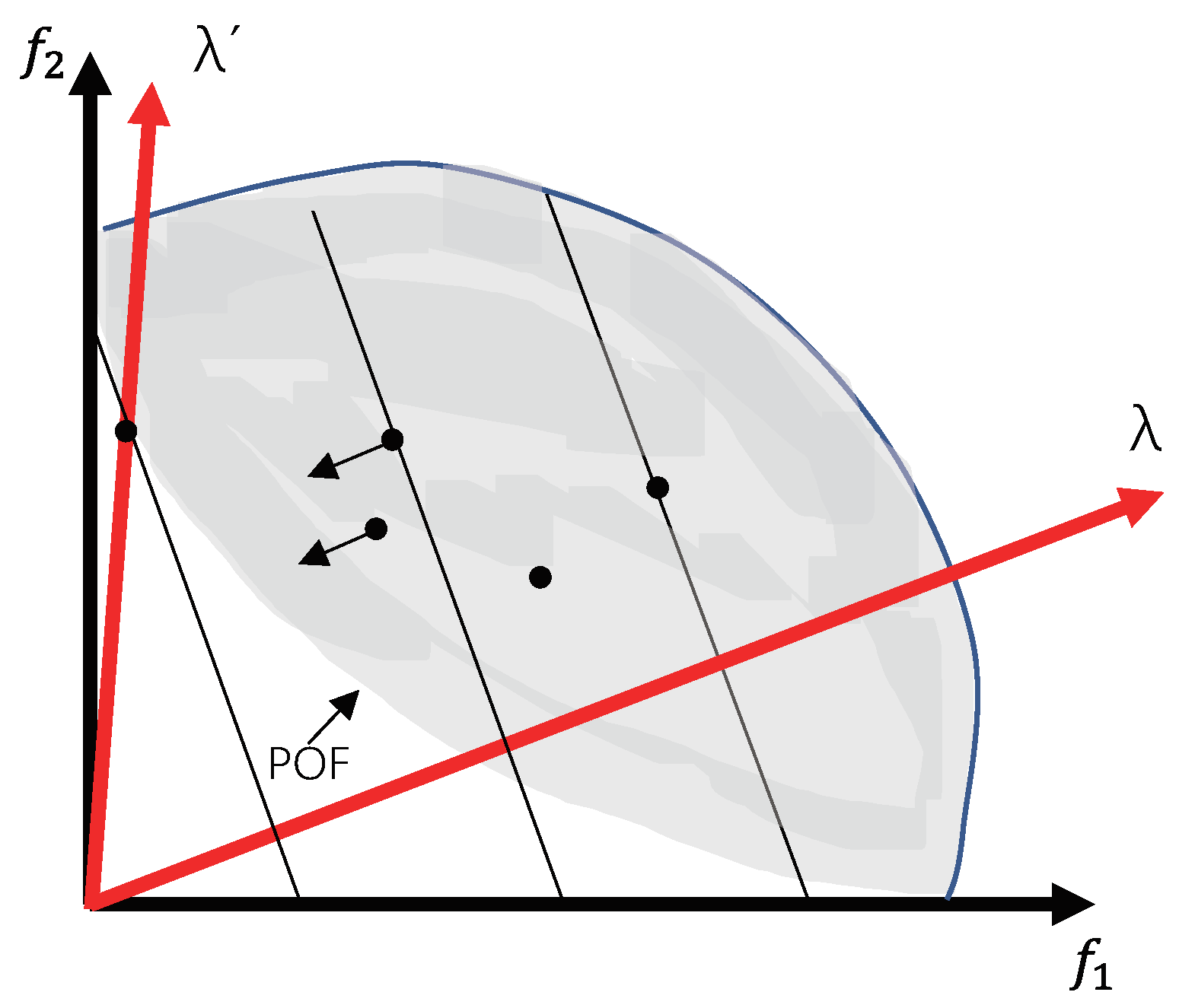
According to the mathematical expression, ✶ can be regarded as the projection of point in the direction of , and finds the minimum value. From the fitness landscape analysis, some contours can be drawn which are perpendicular to , so that we can see that the distance from the origin to the right angle points is the projection of in the direction of . Consequently, discovering that point A is the shortest distance point is not difficult. In the same way, the shortest distance points are found and together produce a different set of Pareto optimal vectors. Nevertheless, the weight summation method has limitations. The standard weight summation method cannot deal with non-convex problems, as shown in Figure 2. For non-convex problems, the perpendicular of each reference vector cannot be tangent to its front edge.
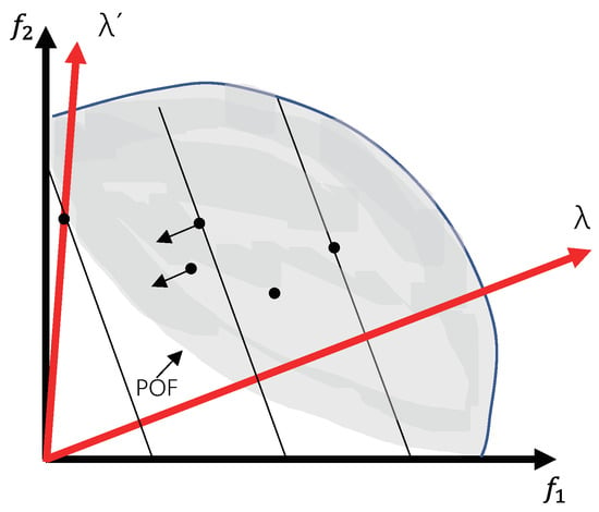
Figure 2.
The contour of weighted sum approach. Concerning convex problems, several isometries can be drawn to discover the shortest distance points that together produce a different set of Pareto optimal vectors. For non-convex problems, the vertical line of each reference vector cannot be tangent to its leading edge. This figure is adopted from [20].
3.1.2. MOEA/D Search Strategy
The MOEA/D algorithm leverages a collaborative optimization approach to solve a single objective or a collection of multiple multi-objective sub-problems, which are derived from the original MOP [70]. The algorithm simultaneously solves all of the sub-problems to identify the entire Pareto front surface. Typically, weight vectors are used to define the sub-problems, and the Euclidean distance between the weight vectors is used to determine the neighborhood relations between sub-problems. The MOEA/D algorithm stands out from other MOEA algorithms due to its focus on selecting parent individuals from the neighborhood, producing new individuals through crossover operations, and carrying out neighborhood population updates by predetermined regulations [71]. Therefore, the neighborhood-based optimization strategy is an integral feature in guaranteeing the search efficiency of MOEA/D. During the evolutionary process, once a high-quality solution for a sub-problem is searched, its good genetic information is rapidly spread to the rest of the individuals in the neighborhood, and it accelerates the rate of algorithm convergence.
The MOEA/D algorithm provides a basic framework using a decomposition strategy, whose most important feature is decomposition and cooperation. Currently, many different versions of the MOEA/D algorithm have been created to address MOP with different difficulty characteristics. In this paper, fundamental MOEA/D algorithms using Chebyshev’s method are presented [72], and its basic data structure is as follows.
- The Chebyshev sub-problem is defined by the set of weight vectors with reference points z.
- Each sub-problem is assigned an individual, and all individuals form a current evolutionary population P.
- The elite population used to save the Pareto solution is EP.
- The sub-problem neighborhood is , .
Unlike other MOEA algorithms, MOEA/D represents an open class of decomposition-based algorithms. Based on MOEA/D, it is easy to combine existing optimization techniques to design efficient algorithms to deal with various problems [46]. For different levels of difficulty that may occur in sub-problems, Zhang et al. presented MOEA/D-DRA with the adaptation of computational resources [73]. MOEA/D considers the simultaneous optimization of multiple single-objective sub-problems, and different sub-problems are responsible for approximating different parts of the Pareto surface, so MOEA/D can be easily parallelized. Nebro and Durillo developed a parallel line-based MOEA/D that can be performed in parallel on multicore computers [74]. Combining the advantages of different aggregation functions, Ishibuchi et al. proposed using different aggregation functions in unused search phases [75]. When dealing with combinatorial optimization problems, optimization for sub-problems can be combined with classical heuristics, e.g., Ke et al. combined MOEA/D with ant colony optimization techniques and suggested the MOEA/D-ACO [76].
3.2. Dominant Relation-Based MOEA Algorithms
3.2.1. Vector Evaluation Genetic Algorithm
To process the target vector, Schaffer proposed the VEGA in 1985 by extending the simple genetic algorithm (SGA). He invented the multi-objective optimization genetic algorithm and provided a Pareto non-inferior solution to the problem utilizing a parallel approach, which resolved the challenging issue of multi-objective optimization that had puzzled the operations research theoretical community [77]. It took the MOGA until the middle and late 1990s to establish a research field and gain success in numerous engineering applications due to computer hardware limitations.
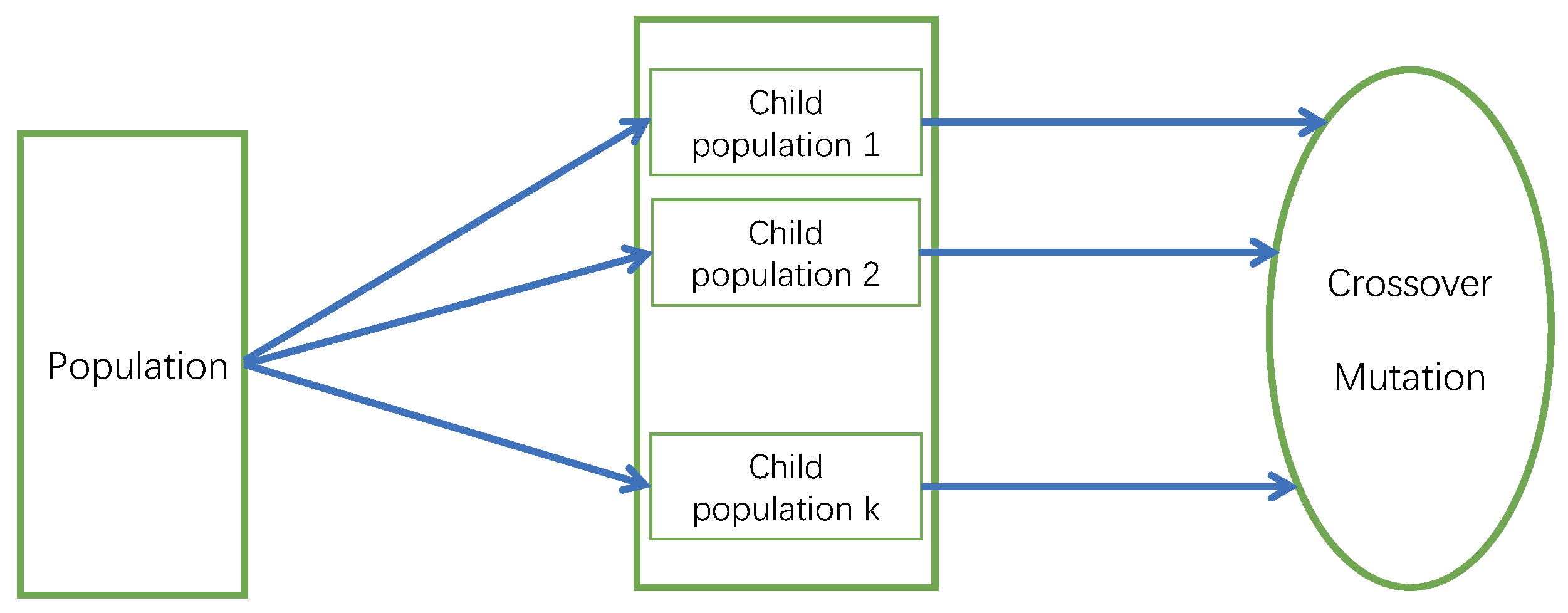
Vector assessment of the genetic algorithm is considered the improved version of the single objective genetic algorithm.It contains some original SGA operators using a proportional selection mechanism. The objective function for each child is produced corresponding to child groups, i.e., it is the objective function [78]. As we observe from Figure 3, the k multi-objective problems need to be assigned into random k groups, and each group size is , where N scales for the whole group. Each sub-objective function evaluates and selects independently in its corresponding sub-groups, and forms a new group to perform crossover and mutation operations. In this way, the process of “segmentation, parallel, evaluation, selection, and merger” proceeds in a cycle, resulting in a non-inferior solution to the problem.
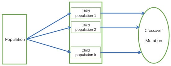
Figure 3.
The operation mechanism of VEGA. The MOP is divided into groups, each sub-objective function is evaluated and selected independently, then a new group is formed, crossover and variation operations are performed, and this proceeds cyclically, resulting in non-inferior solutions to the problem. This figure is adopted from [5].
3.2.2. Lexicographic Optimization Method
In the study of MOEA algorithms using dominance relation, lexicographic optimization is a class of multi-objective optimization algorithms that identify the solution to the Pareto front. It starts by considering an objective function and determines the feasible domain of the objective space using other functions as constraints [79]. Depending on their essentialness or significance, the objective functions are identified and optimization is carried out iteratively. Single-objective optimization can more easily find the optimum because only one objective function is considered. However, since multi-objective optimization attempts to search for the Pareto optimal solutions, the use of lexicographic optimization allows multiple objective functions simultaneously aiming for the Pareto optimal solutions.
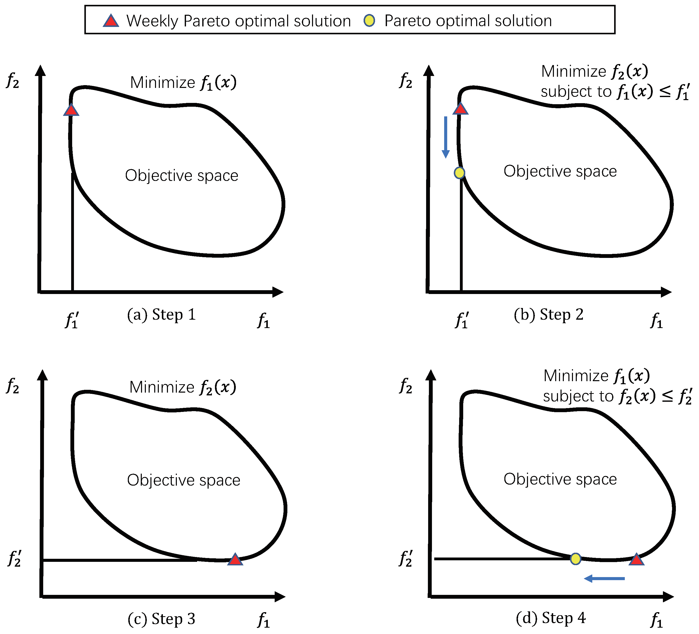
Figure 4 presents an example of the lexicographic optimization process for a bi-objective minimum optimization problem, where and are the objective functions and and are the optimal solutions of two objective functions, respectively. To prevent finding the weak Pareto optimum solution, the objective functions are minimized in turn, while the solutions achieved are employed as constraints. The Pareto optimum solution is discovered using the optimal value of one objective function as a constraint after the other objective functions have been minimized. In this way, if there are n objective problems, n initial best solutions of each objective function can be available as the beginning point for finding the next Pareto optimal solution of the objective function that is currently optimized.
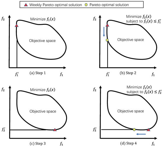
Figure 4.
An example of the lexicographic optimization process for a bi-objective minimum optimization problem. Firstly, is minimized, while the optimal value obtained is used as a constraint. Secondly, after has been minimized, its optimal value is used as a constraint for cyclic optimization. Finally, Pareto optimal solutions are found. This figure is adopted from [80].
3.2.3. Niched Pareto Genetic Algorithm
Based on the Pareto dominance connection, Horn et al. propounded the NPGA [7]. It randomly selects two individuals i and j from the population, randomly selects a comparing set CS (whose size is larger than two and generally smaller than ten), and compares individual i and individual j with the individuals in CS, respectively. If one of the individuals is dominated by the CS and the other is not dominated by the CS, the individual that is not dominated by the CS will be chosen to be involved in the next generation of evolution, and if both individuals i and j are not dominated by the CS or both are dominated by the CS, then the individual with the greater shared fitness will be selected to participate in the next generation of evolution using a sharing mechanism.
Fitness sharing is an effective way to achieve population diversity. Let the fitness of individual i be , the niche count of individual i be , and is calculated as follows in Equation (3):
The P is the current evolutionary population, is the distance or similarity between individual i and individual j, the sharing function is , and is defined as follows in Equation (4):
The niche radius is , usually determined by the user based on the minimum desired spacing between individuals in the optimal solution set.
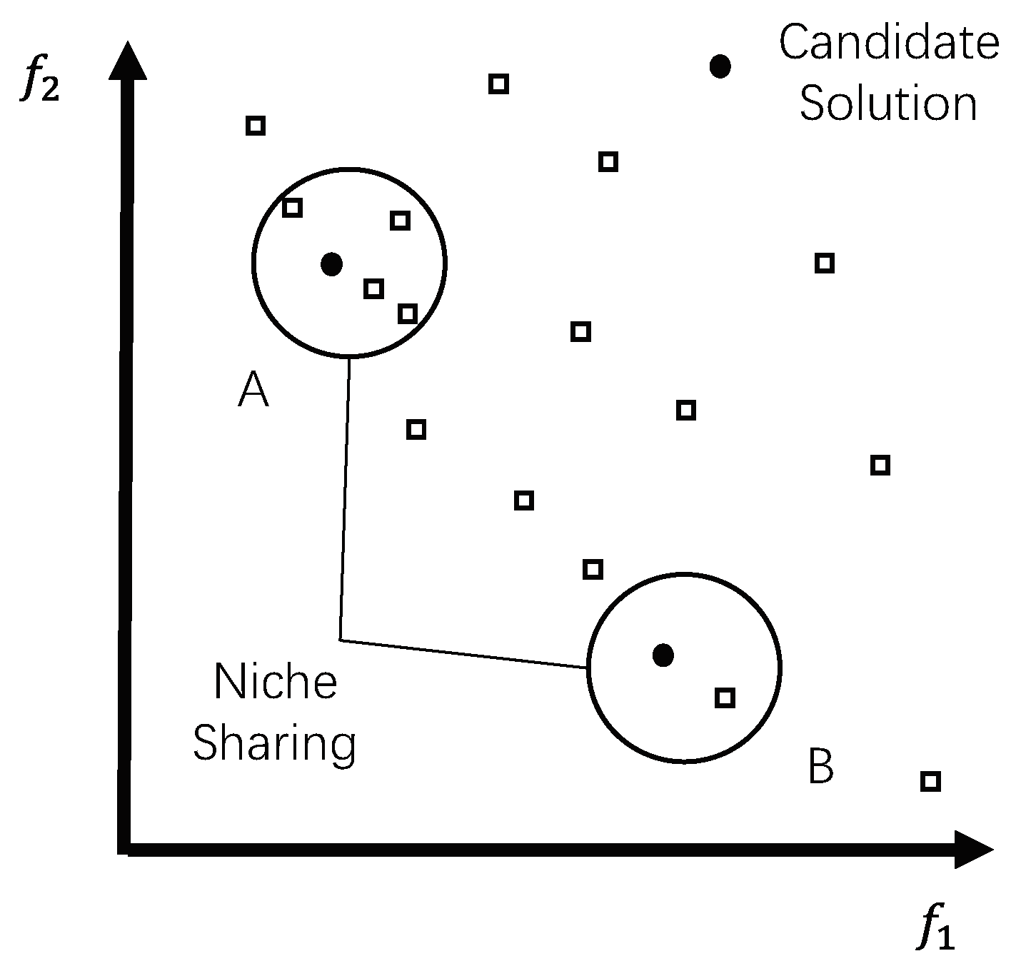
Define as the shared fitness, where is essentially the degree of niche aggregation of individual i. Individuals within the same niche reduce each other’s shared fitness. The higher the degree of aggregation of an individual, the more its shared fitness relative to its fitness is reduced. As shown in Figure 5, candidate solutions A and B are both non-dominated, but A has a greater degree of aggregation than B, and therefore A has a smaller shared fitness than B. The purpose of using shared fitness is to spread the evolutionary population over distinct areas throughout the entire search space.
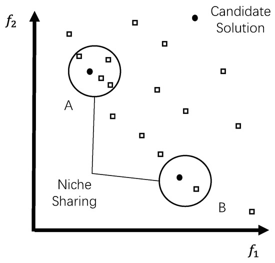
Figure 5.
The niche sharing. Neither candidate A nor B is dominant, but A is more aggregated than B, so A has less shared fitness than B and chooses B to participate in the next generation of evolution. This figure is adopted from [7].
The main advantage of the NPGA is that it operates more efficiently and achieves a better Pareto optimality boundary. The disadvantage is the difficulty in selecting and adjusting the radius of the niche [81].
3.2.4. Non-Dominated Sorting Genetic Algorithm II
In 1993, Srinivas and Deb presented the NSGA. There are three key issues with the NSGA. The first is the absence of an ideal individual retention mechanism. Studies of relevance indicate that, for one thing, the performance of MOEA can be improved and the loss of exceptional solutions can be avoided by using the best individual retention mechanism. The issue of common parameters is the second issue. If shared parameters are employed during the evolution process to preserve population distribution, it might be challenging to estimate their size as well as dynamically modify and adapt parameters. Thirdly, one challenge with the Pareto optimal solution set is that it requires a high time complexity to construct, with a cost of O(R×), where R is the number of objectives and N is the size of the evolutionary population. This can be problematic because each generation of the evolution process involves constructing a non-dominated set, which can be time-consuming when the size of the evolutionary group is large. To address this issue, the NSGA-II algorithm is proposed as an improvement upon the NSGA algorithm [16].
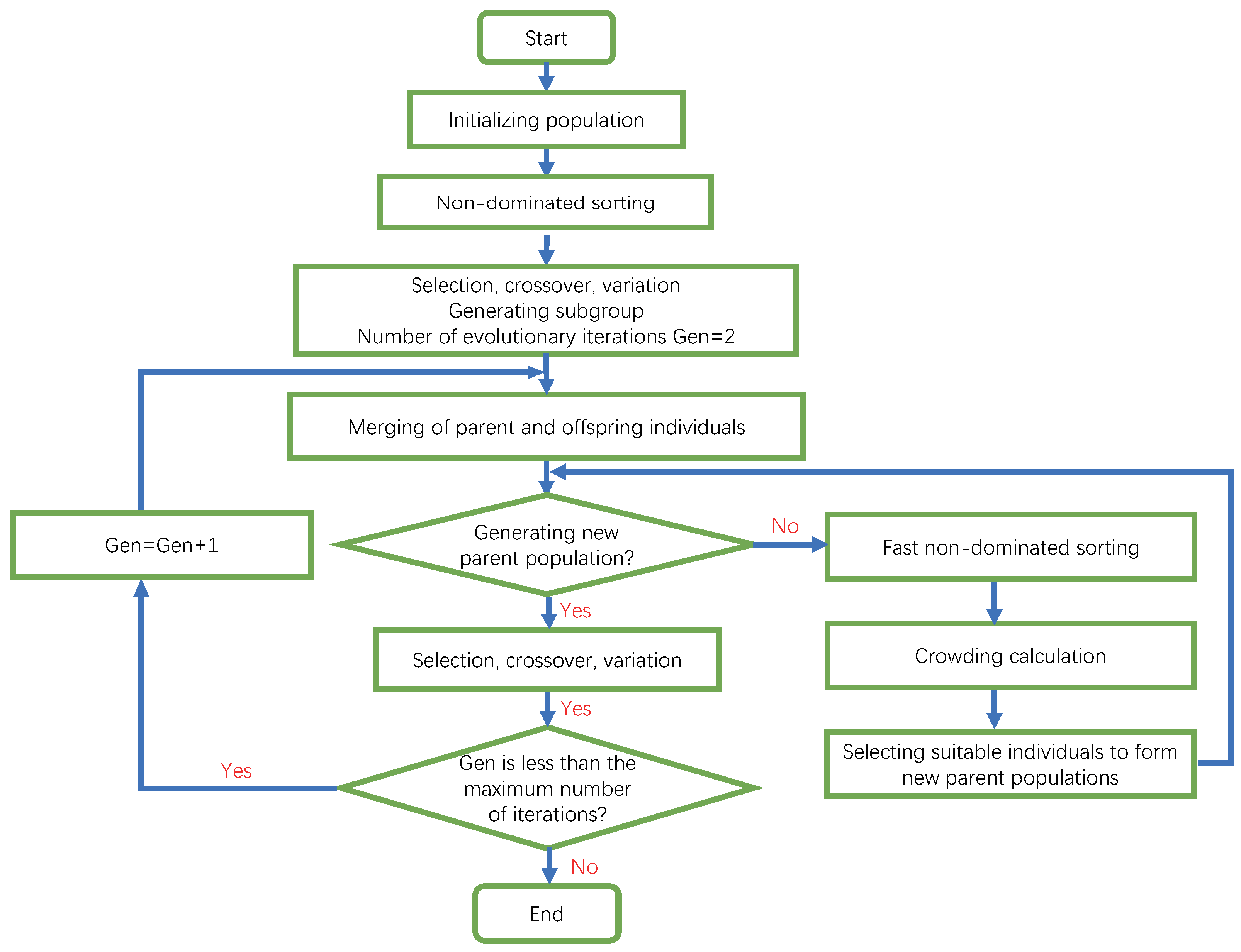
The NSGA-II algorithm’s fundamental concept is as follows. Following non-dominated sorting, the random preliminary population of size N is produced, and the three fundamental genetic algorithm processes of selection, crossover, and mutation are used to create the first generation of the offspring population. Starting with the second generation, the parental and child populations were mixed to accomplish a rapid non-dominant ranking. The crowding distance of individuals in each non-dominant layer was also determined at this time [82]. To create the new parent population, individuals are selected based on their non-dominant relationship and crowding distance. The standard genetic algorithm operations are performed to produce the new child population. This process is repeated until the end condition of the program is met. The program flow chart for this process is depicted in Figure 6.
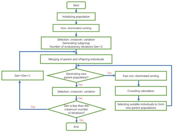
Figure 6.
The fundamental concept of the NSGA-II algorithm. A random initial population, using selection, crossover, and variation to produce a first generation of offspring populations. Parent and offspring populations are mixed and individuals are selected for new parent populations based on their non-dominance relationships and crowding levels, which in turn produce new offspring populations. This figure is adopted from [16].
Fast Non-Dominated Sorting Algorithm
To perform non-dominant sorting, the algorithm must determine two parameters, and , for each individual in the population . represents individual accounts that dominate individual [83], and is the group of individuals dominated by in the population. When traversing the entire population, the combined computational complexity of these two parameters is . The steps to implement the fundamental and formal computational procedure for non-dominant sorting are as follows:
- Select the first individual to be the current individual.
- Compare the current individual’s objectives with all the other individual’s objectives.
- Count the individual accounts that dominate the current individual, which is represented by .
- Set the individuals who satisfy the condition as the first front and temporarily delete them from the generation for the time being.
Adopt Congestion Degree and Congestion Comparison Operator
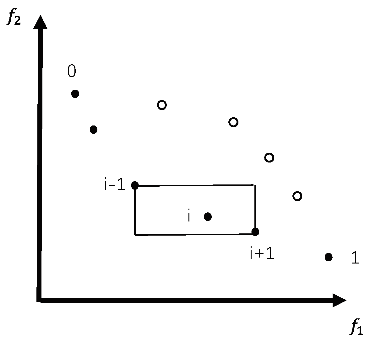
(1) Crowding degree estimation [84]: To assess the degree of crowding around a solution in the population, the mean distance between the two dots on each side of a particular point is computed according to each objective function. The vertex of the cuboid is determined by its nearest neighbor, and the number is utilized to determine its circumference (called the crowding factor). The length of the cuboid surrounding the i-th solution’s front surface is equal to the solution’s crowding coefficient (as shown in the dotted box) in Figure 7. The calculation of the degree of crowding ensures that the population is diverse. The population must be sorted for the crowding coefficient computation using the values of each objective function in ascending sequence. As a result, for each objective function, the infinite distance value is called the boundary solution, which has the maximum and lowest values. The value for all other intermediate solutions is given as the absolute difference between the normalized values of the two nearby solutions. The other objectives have the same objectives. The distance values for each objective are added to determine the crowding coefficient values. Every objective function is normalized before the congestion factor is calculated.
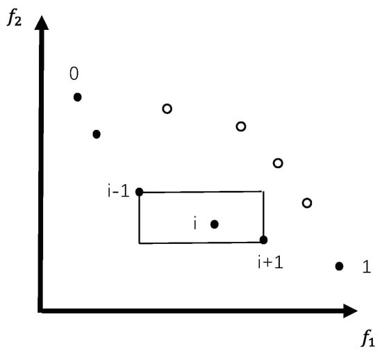
Figure 7.
The crowding distance about the i-th solution. The average distance between the two points on either side of point i is calculated; based on each objective function, the vertices of the rectangle are determined by their nearest neighbors, i.e., and , and the length of the cube is equal to the congestion factor of the solution in the graph. This figure is adopted from [16].
(2) Crowding comparison operator [85]: After performing the quick non-dominant ranking and crowding calculation, each individual i has two properties. The non-dominant ranking, i_{rank} (the rank) and the crowding, i_{d}. These properties can be used to define a congestion comparison operator for comparing individual i with another individual j. Either of the following is true and will result in an individual i winning. If the non-dominant stratum of individual i is higher in the ranking than the non-dominant stratum of individual j, i_{rank} < j_{rank} If in the same non-dominant layer and the crowding distance of individual i is greater than that of individual j, i.e., i_{rank} = j_{rank} and i_{d} > j_{d}.
The first requirement is to ensure that the selected individuals have a higher non-dominated rank. The second condition is to choose a region with low congestion when two individuals are tied to the same non-dominant layer according to their crowding distance. The winner can proceed to the next operation.
The NSGA-II algorithm introduces an elite strategy to retain good individuals to eliminate the inferior ones. The elite strategy expands the screening range when generating the next generation of individuals by mixing the parent and offspring individuals to form a new population. Analyzing the example shown in Figure 8, where P denotes the parent population, let the individual accounts in it be , and the denotes the offspring population. The steps are as follows.
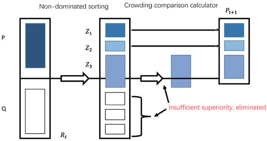
Figure 8.
The implementation steps for NSGA-II’s elite strategy. The new population is ranked non-dominantly; in this example, the population is divided into six Pareto ranks, and non-dominant individuals with Pareto rank 1 and 2 are placed in a new set of parents, after which their crowding is determined before ranking those with Pareto rank 3 and excluding all those with ranks 4 to 6. This figure is adopted from [16].
Elitism
- Create a new population by merging parental and child populations. After that, the new population is sorted non-dominantly, and in this case, the population is divided into six Pareto classes.
- To generate a new parent population, non-dominated individuals having Pareto rank 1 are placed in a new parent collection, and then the individuals with Pareto rank 2 are added to the new parent population, and so on.
- The crowding degree is calculated for all the individuals with rank , if there are fewer individual accounts in the set than before all individuals with rank are added to the new parent set, but individual accounts in the set increase after all individuals with rank are added. All individuals with ranks more than are deleted after these people are ranked according to how crowded they are. Since in this illustration is 2, one must determine the degree of crowding among those with Pareto rank 3 before ranking them and excluding everyone with ranks 4 to 6.
- Place the individuals in rank in the new set of parents one by one in the order ranked in step 2 until individual accounts in the parent set up to and the remaining individuals are eliminated.
3.3. Evaluation Index-Based MOEA Algorithms
Evaluation indexes are quantitative tools for assessing the performance of different MOEAs, which can be divided into three categories: convergence, distribution, and comprehensiveness [86]. One immediate idea is to integrate metrics into MOEA to guide the evolutionary search process of MOEA. Theoretically, any metrics can be incorporated into MOEA in a variety of ways, but several metrics, such as spacing (SP) [87], generational distance (GD) [88], and inverted generational distance (IGD) [89] can make the algorithm more complex when integrated into MOEA. It may reduce the operating efficiency of MOEA, but it cannot improve the distribution performance and convergence performance of MOEA. Researchers embedded hypervolume(HV) into MOEA and proposed an S-Metric selection-based evaluative multi-objective optimization algorithm (SMS-EMOA) which can effectively solve MOP [90]. Zitzler and Künzli, successfully embedded a HV and binary -indicator evaluation index into MOEA as a fitness evaluation method and proposed an indicator-based evolution algorithm (IBEA) which improved the performance of MOP solution [91].
3.3.1. S-Metric Selection Based Evaluative Multi-Objective Optimization Algorithm
We will introduce HV in Section 4. Zitzler and Thiele first suggested the HV metric, also referred to as the S-metric, and they referred to it as the size of the coverage space or the dominated space. As a crude approximation to the Pareto frontier, the EMO method produces a set of points in the performance space. To calculate how close the predicted data points are to the real Pareto front, quantitative measures are needed [92]. The HV indicator, which estimates the HV between the Pareto front (P) and the reference point (R), is one of these measurements.
As shown in Figure 9, a key characteristic of SMS-EMOA is that it updates using a steady-state strategy in which a single offspring is generated in each iteration and immediately evaluated before being integrated into the evolution of the next generation. This means that each generation only produces one new person. Algorithm 1 describes the basic algorithm, starting from the initial population, using a random mutation operator to generate a new individual [93]. Unlike some other methods for maintaining a collection of non-dominant individuals, SMS-EMOA maintains a constant population size for both dominant and non-dominant individuals. To decide which individuals are removed during the selection process, it is necessary to set the parameter selection in the dominant solution.
| Algorithm 1 SMS-EMOA |
|

Figure 9.
The operation mechanism of the SMS-EMOA algorithm. An offspring is produced in each iteration and evaluated immediately before integration into the next generation of evolution, with poor individuals being eliminated as a new subpopulation. This figure is adopted from [90].
Algorithm 2 describes a replacement program that reduces employment. To select the individuals that make up the population, SMS-EMOA uses a ranking system based on the Pareto frontier, a concept derived from the well-known NSGA-II algorithm.
- The fast non-dominant sorting algorithm is used to calculate the Pareto front of the non-dominant level until cannot be put down in the population G (put the parent generation (N individuals) and the offspring (N individuals) together, then selects the first N better individuals).
- After that, an individual is dropped from the worst ranking. If front contains || > 1 (domination of the individual is greater than an individual, then for s ∈ layer included in the Pareto frontier s) of the individual will be eliminated, minimize it.The △S (s, ) represents the HV of s. The smaller the HV, the smaller the role of this individual should be removed. The point with the worst non-dominant leading edge is selected in each of the two objective functions and ranks them by the original objective function ’s value. We then receive a second sequence that is arranged according to , because none of these points dominates the others. △S (s, ) is calculated as follows in Equation (5). For : = {... s ||}
The SMS-EMOA algorithm is a promising Pareto optimization algorithm. It is especially useful when a few solutions are needed and a balanced solution is important. However, it has a high selection time complexity and is typically only applied when there is only one layer of the non-dominant level [94]. Despite this, SMS-EMOA tends to produce good results.
| Algorithm 2 Reduce(Q) |
|
3.3.2. Indicator-Based Evolution Algorithm
Zitzler and Künzli proposed a generalized evolutionary model in 2004, which first proposed IBEA by embedding the evaluation indicator function as an adaptation evaluation method in MOEA. The rating indicator function is formally defined as a function that maps a group of vectors to a group of real numbers. In other words, it is a mathematical function that allocates a numerical value to a vector I, ; using the all-order relationship on the set of real numbers, it is possible to compare the quality between different sets of vectors in F space. In IBEA, a simpler way of assigning fitness is specified as follows.
where k is a scaling factor greater than 0 and I is a real number function that maps the group of Pareto approximation solutions in the objective space to a group of real numbers in Equation (6). In this context, it is defined in Equation (7):
As shown in Figure 10, A and B are two solution sets containing only one individual, respectively. In (a), when the individuals in set and the individuals in the group are not dominated by each other, the left yellow part indicates the area of the independently dominated region of set A, then there is . The red part indicates the area of the independently dominated region of set B, and there is . In (b), the gray part of the figure indicates the area of the independently dominated region of set B, then there is , and .
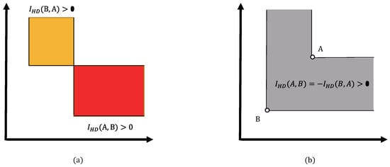
Figure 10.
The illustrations of indicator. In (a), when the individuals in the set and the individuals in the set are not dominated by each other, the yellow and red parts on the left indicate the areas of the independently dominated regions of and , respectively. In (b), when is dominated by , the gray part of the figure indicates the area of the independently dominated region of . This figure is adopted from [91].
By iteratively eliminating the most poorly performing individuals in the population and adjusting the fitness values of the remainder, Algorithm 3 performs mating selection and environmental selection.
| Algorithm 3 IBEA |
|
3.4. High-Dimensional MOEA
In multi-objective optimization studies, the difficulty of optimization increases exponentially with the increasing number of objective dimensions. Usually, optimization problems with four or more objectives are called high-dimensional multi-objective optimization problems. In recent years, high-dimensional MOEA has become a highly popular research topic in the field of evolutionary multi-objective optimization. Classical MOEAs, such as NSGA-II and SPEA2, have good results in solving two-dimensional or three-dimensional optimization problems. However, as the number of objective dimensions increases, these classical MOEAs based on Pareto dominance relations face many difficulties.
- Degradation of the search capability. As the number of objective dimensions increases, the number of non-dominated individuals in the population increases exponentially, thus reducing the selection pressure of the evolutionary process.
- The number of non-dominated solutions used to cover the entire Pareto front increases exponentially.
- Difficulties in visualizing the optimal solution set.
- The computational overhead for evaluating the distributivity of the solution set increases.
- The efficiency of the recombination operation decreases. In a larger high-dimensional space, the children resulting from the recombination of two distant parents may be far away from the parents, making the ability of the local search of the population weaker. Therefore, designing and implementing algorithms that can efficiently solve high-dimensional multi-objective optimization problems is one of the current and future challenges in the field of evolutionary multi-objective optimization.
In recent years, scholars have proposed some effective methods for solving high-dimensional multi-objective optimization problems. One type of algorithm is based on Pareto dominance relations, which reduce the number of non-dominated individuals by extending the Pareto dominance region, such as -MOEA [95] and control the dominance area of solutions (CDAS) [96]. An aggregation function can also be used to aggregate multiple objectives into a single objective for optimization, such as MOEA/D, NSGA-III [97], and MSOPS-II [98]. Finally, there are metric-based algorithms that use performance evaluation metrics to compare the merits of two populations or between two individuals, such as IBEA, SMS-EMOA, and Hyp [99]. In 2013, Li Miqing proposed a shift-based density estimation method (SDE) from the perspective of a diversity retention mechanism and integrated it into SPEA2 with good results [100]. In addition, one scholar dealt with the high-dimensional multi-objective optimization problem by trying to reduce the number of objectives, and the treatment methods mainly include the principal component analysis method [101], the redundant objective elimination algorithm based on the minimum objective subset [102]. Reducing redundant objectives or unimportant objectives is also an important direction for high-dimensional MOEA research.
4. Evaluation Metrics of MOEA
4.1. Evaluation Settings
In the design and implementation process of MOEA, efforts should not only be put into determining appropriate tests and designing appropriate experiments but also selecting reliable test tools, as well as performing corresponding statistical evaluation and comparative judgment. To assess the capability of MOEA algorithms and, at some level, facilitate the search for optimal solutions, researchers often use certain standard test functions. Comprehensive evaluation indices, such as HV and IGD, are commonly employed to gauge the convergence, uniformity, and diversity of the Pareto solutions generated by an EMO algorithm. These indices provide a scalar value that reflects both the convergence and distribution of the solutions simultaneously. The number and variety of Pareto solutions resulting from the algorithm are also important factors to consider.
4.2. Multi-Objective Optimization Benchmark Problems
Multi-objective algorithms require a test function to test the capability of the algorithm when it is improved. The test function needs to be capable of reflecting or containing the basic features of the MOP, such as continuous or discontinuous, derivable or non-derivable, convex or concave, single-peaked or multi-peaked, deception problem or non-deception problem, etc. The widely used benchmark multi-objective test functions are MOP1~MOP7, MOP-C1~MOP-C5 with bias constraints, ZDT1~ZDT6, and DTLZ1~DTLZ7, etc. [103]. This paper focuses on the ZDT test functions that are extensively employed in the evaluation of multi-objective algorithms. To assess the optimization capabilities of MOEA, we consistently employ five multi-objective benchmark problems known as ZDT functions, as demonstrated in Table 2, to evaluate its performance.

Table 2.
Evaluation is conducted using a multi-objective benchmark function. for the whole Pareto frontier.
Zitzler et al. proposed the set of ZDT test functions in 2000, which is currently the most widely used set of multi-objective test functions [103]. It includes DZT1~DZT6, six different forms of test functions. They are characterized by the following two points:
- (1)
- All of the functions have two objective functions, . Additionally, the plotted graph is straightforward to grasp because the form and position of the Pareto optimal frontier are known.
- (2)
- The number of decision variables is highly flexible and can be varied as needed.
4.3. Hyper-Volume Indicator
The application of the HV index in the scope of evolutionary algorithms is widespread due to its strong theoretical foundation. By calculating the HV value of the space bounded by the reference point and the non-dominated solution set, the overall performance of MOEA was assessed. The non-dominated solution set and the reference point of the multi-objective optimization algorithm measure the volume of the objective space, and this volume is measured by the HV index. The HV as shown in Equation (8) is a measure of quality that is strictly monotonic for Pareto dominance. In this equation, the volume is measured using the Lebesgue measure, represented by the . The count of elements of the non-dominated solution set is represented by the symbol |S|, and the hypercube created by the reference point z∗ and the i-th solution in the solution set is represented by the . A higher HV value indicates an algorithm with superior performance.
However, there are two defects with HV. First, the HV index is calculated over a long period. Second, the choice of reference points influences the HV index’s accuracy to some amount.
4.4. Inverted Generational Distance Indicator
The generation distance is the average distance between all individuals in the algorithm’s non-dominated solution set and the Pareto-optimal solution set, whereas the inversion generation distance is the generation distance’s reverse mapping [104]. The IGD index, as shown in Equation (9), is a measure of the overall capability of the algorithm. It primarily determines the smallest distance sum between each point on the actual Pareto frontier and the particular set that the algorithm produced. It is employed to assess the algorithm’s capability in respect to convergence and distribution. The overall performance improves as the value decreases. In this equation, the group of point p is evenly distributed across the actual Pareto surface. The quantity of points dispersed across the actual Pareto surface is denoted by |p|. The procedure yielded the optimal Pareto solution set Q, and the minimum Euclidean distance between individual v and population Q.
The IGD index cannot only evaluate the convergence of MOEA but also assess its distribution uniformity and universality.
5. Discussions on Perspective Studies
Multi-objective optimization aims to discover all Pareto optimal solutions. The multi-objective optimization is generally considered an NP-complete problem. To successfully optimize using evolutionary computation [105], there are three main challenges:
- (1)
- Ensuring that the population moves toward the real Pareto-optimal front.
- (2)
- Giving the developed solutions a fitness rating and choosing which ones should take part in mating to produce the population of the following generation. Due to the existence of non-comparable individuals, this is a challenging task.
- (3)
- A fairly decentralized trade-off front is achieved by maintaining the diversity of the population and preventing premature convergence. This should be ensured up until the algorithm converges by approaching the Pareto front, as population diversity allows for the retention of potentially efficient solutions.
In our prior study, we examined the MOCE algorithm’s performance during optimization utilizing several chaotic system implementations [106]. The evaluation’s findings show that various chaotic systems do indeed affect optimization performance, and this work shows that the MOCE using the logistic map outperforms the others in this regard.
In the evolution process of the population, the genetic algorithm adopts a completely random search method. Moreover, there is almost no necessary connection between generations except for the control of parameters like crossover and mutation probability [107]. Although this model is useful in practical applications, it has problems of low efficiency, such as premature convergence and slow convergence. On the other hand, from the perspective of chaos, the mode of biological evolution is “random + feedback”, in which the randomness is caused by the inside of the system and is the feature of the system itself, and chaos is the source of system evolution and information. Compared with the traditional model, this biological evolution model is closer to the real biological evolution model. Therefore, the genetic algorithm that introduces chaos will have better results. We present a newly population-based optimization approach called chaotic evolution that makes use of the traversal characteristics of chaos for the exploration and utilization functions of evolutionary algorithms. Through the use of straightforward concepts, CE replicates ergodic motion in the search space and adds mathematical processes to the iterative evolution process. A general search capability exists in the general genetic algorithm. By incorporating different chaotic systems into the CE algorithm architecture, it is simple to increase its search capacity. Compared to certain other evolutionary computing algorithms, CE is more scalable [108]. To evaluate the qualities of the suggestions, many surveys and comparative evaluations were carried out. Our findings can improve optimization performance as compared to the evolutionary algorithm itself by optimizing the chaotic evolutionary algorithm.
On the other hand, it is the visualization research algorithm of the chaotic evolutionary algorithm [109]. Algorithm visualization abstracts the code, operation, and semantics of the program, and displays these abstractions dynamically. Taking the sorting algorithm as an example, the algorithm visualization system will first combine and abstract the code in the program, convert assignment and loop statements into element exchange and insertion operations in the sorting algorithm, and then when the program executes these statements, the system will for the corresponding operation and display the corresponding animation in the sorting algorithm. Algorithm visualization does not visualize each statement and it focuses on the logic and algorithm expressed by the statement as a whole. Algorithms have knowledge-based concepts such as algorithm ideas and algorithm processes. One task of algorithm visualization is to visualize the knowledge involved in the algorithm to make it easier to understand, disseminate and communicate. As for our chaotic evolutionary algorithm, its visualization research is also essential to work. Through visualization, researchers can quickly establish the connection between the algorithm and the code, and improve their programming ability.
Finally, a systemic optimization approach called interactive evolutionary computation (IEC) uses the subjective of a real human evaluation to accelerate optimization [110]. There are numerous tasks whose performance can be assessed by humans, but is difficult to gauge, or nearly impossible to quantify by machines. In some real-world system optimization problems, it may not be easy to devise a fitness function that accurately reflects the subjective evaluation of a real person. To address this challenge, a real person is used instead of the fitness function, allowing the problem to converge to the subjective evaluation of the real person. IEC searches in two different places. By the distance of F mental space between the objective and the system output, human users assess the output of the objective system. Meanwhile, the evolutionary algorithm searches in the parameter space. IEC can be thought of as an optimization strategy that relies on the mapping between these two spaces, where manual search and evolutionary algorithms are combined.
6. Conclusions and Future Works
In this study, three categories of MOEA algorithms are described in depth. Decomposed multi-objective optimization methods fall under the first category. These algorithms divide the original MOP into a few simpler MOP or single-objective optimization problems that can be solved in a group setting. The MOEA based on Pareto domination is the second type, which uses a Pareto-dominated mechanism based on which candidate solutions are distinguished and selected [50]. The third category is index-based MOEA, which uses the performance index of solution quality measures as the choice criterion in the environment options. Each of these three MOEA algorithms has its advantages and disadvantages. We believe that it is our research direction to try to combine them in order to see if chaotic evolutionary algorithms can improve the optimization capabilities of each of these algorithms.
In our previous studies, we have thoroughly examined a range of algorithms for solving the MOP, and have provided explanations and analyses of several solutions. Our future research will primarily concentrate on the following aspects:
- (1)
- Each representative algorithm mentioned in this paper is coded in conjunction with chaotic evolution, and then the results are compared and analyzed under the same experimental conditions, and finally summarized.
- (2)
- The visualization research of chaotic evolutionary algorithms is also one of the most important works in this field [111]. To carry out better visualization research, enough knowledge of the content and core of the algorithm is necessary. Based on this previous research, we can visualize it in order to make it intuitive and easier to understand, disseminate, and communicate. In addition, visual research is also related to the interaction of MOCE for displaying and interacting with users.
- (3)
- Any population-based evolutionary algorithm that does not rely on exploring spatial information can be used as an algorithmic framework for interactive evolutionary computation. Each of the different algorithms has its algorithmic properties. For interactive evolutionary calculations with few evolutionary iterations and limited population size, the algorithm to show high optimization performance is ideal for applications with interactive evolutionary computing [112]. Therefore, one of the directions of our research is to explore the potential of interactive MOCE. In future studies, it would be good to investigate whether the interactive MOCE algorithm would have better optimization capabilities using these search strategies investigated in this paper.
Author Contributions
Z.W. and Y.P. contributed equally to this paper. Conceptualization and methodology, Z.W. and Y.P; validation, Z.W. and Y.P and J.L.; formal analysis, Z.W. and Y.P; investigation, Z.W.; resources, Z.W. and Y.P. and J.L.; writing—original draft preparation, Z.W.; writing—review and editing, Z.W. and Y.P. and J.L.; supervision, Y.P. and J.L. All authors have read and agreed to the published version of the manuscript.
Funding
This research received no external funding.
Institutional Review Board Statement
Not applicable.
Informed Consent Statement
Not applicable.
Data Availability Statement
Not applicable.
Conflicts of Interest
The authors declare no conflict of interest.
References
- Coello, C.C. Evolutionary multi-objective optimization: A historical view of the field. IEEE Comput. Intell. Mag. 2006, 1, 28–36. [Google Scholar] [CrossRef]
- Deb, K. Multi-Objective Optimization Using Evolutionary Algorithms: An Introduction. In Multi-Objective Evolutionary Optimisation for Product Design and Manufacturing; Springer: London, UK, 2011; pp. 3–34. [Google Scholar]
- Shao, Y.; Lin, J.C.W.; Srivastava, G.; Guo, D.; Zhang, H.; Yi, H.; Jolfaei, A. Multi-Objective Neural Evolutionary Algorithm for Combinatorial Optimization Problems. IEEE Trans. Neural Netw. Learn. Syst. 2021, 34, 2133–2143. [Google Scholar] [CrossRef] [PubMed]
- Schaffer, J.D. Some Experiments in Machine Learning Using Vector Evaluated Genetic Algorithms; Technical Report; Vanderbilt University: Nashville, TN, USA, 1985. [Google Scholar]
- Srinivas, N.; Deb, K. Multiobjective optimization using nondominated sorting in genetic algorithms. Evol. Comput. 1994, 2, 221–248. [Google Scholar] [CrossRef]
- Fonseca, C.M.; Fleming, P.J. Genetic Algorithms for Multiobjective Optimization: Formulation, Discussion and Generalization. Icga 1993, 93, 416–423. [Google Scholar]
- Horn, J.; Nafpliotis, N.; Goldberg, D.E. A niched Pareto genetic algorithm for multiobjective optimization. In Proceedings of the First IEEE Conference on Evolutionary Computation, Orlando, FL, USA, 27–29 June 1994; pp. 82–87. [Google Scholar]
- Li, Z.; Zou, J.; Yang, S.; Zheng, J. A two-archive algorithm with decomposition and fitness allocation for multi-modal multi-objective optimization. Inform. Sci. 2021, 574, 413–430. [Google Scholar] [CrossRef]
- Zitzler, E.; Thiele, L. An evolutionary algorithm for multiobjective optimization: The strength Pareto approach. TIK Rep. 1998, 43. [Google Scholar] [CrossRef]
- Zitzler, E.; Laumanns, M.; Thiele, L. SPEA2: Improving the strength Pareto evolutionary algorithm. TIK Rep. 2001, 103. [Google Scholar] [CrossRef]
- Knowles, J.D.; Corne, D.W. Approximating the nondominated front using the Pareto archived evolution strategy. Evol. Comput. 2000, 8, 149–172. [Google Scholar] [CrossRef] [PubMed]
- Corne, D.W.; Knowles, J.D.; Oates, M.J. The Pareto envelope-based selection algorithm for multiobjective optimization. In Proceedings of the International Conference on Parallel Problem Solving from Nature, Paris, France, 18–20 September 2000; pp. 839–848. [Google Scholar]
- Corne, D.W.; Jerram, N.R.; Knowles, J.D.; Oates, M.J. PESA-II: Region-based selection in evolutionary multiobjective optimization. In Proceedings of the 3rd Annual Conference on Genetic and Evolutionary Computation, San Francisco, CA, USA, 7–11 July 2001; pp. 283–290. [Google Scholar]
- Erickson, M.; Mayer, A.; Horn, J. The niched Pareto genetic algorithm 2 applied to the design of groundwater remediation systems. In Proceedings of the International Conference on Evolutionary Multi-Criterion Optimization, Zurich, Switzerland, 7–9 March 2001; pp. 681–695. [Google Scholar]
- Coello, C.A.; Pulido, G.T. Multiobjective optimization using a micro-genetic algorithm. In Proceedings of the 3rd Annual Conference on Genetic and Evolutionary Computation, San Francisco, CA, USA, 7–11 July 2001; pp. 274–282. [Google Scholar]
- Deb, K.; Pratap, A.; Agarwal, S.; Meyarivan, T. A fast and elitist multiobjective genetic algorithm: NSGA-II. IEEE Trans. Evol. Comput. 2002, 6, 182–197. [Google Scholar] [CrossRef]
- Fei, Z.; Li, B.; Yang, S.; Xing, C.; Chen, H.; Hanzo, L. A survey of multi-objective optimization in wireless sensor networks: Metrics, algorithms, and open problems. IEEE Commun. Surv. Tutor. 2016, 19, 550–586. [Google Scholar] [CrossRef]
- Coello, C.C.; Lechuga, M.S. MOPSO: A proposal for multiple objective particle swarm optimization. In Proceedings of the 2002 Congress on Evolutionary Computation, CEC’02, Honolulu, HI, USA, 12–17 May 2002; Volume 2, pp. 1051–1056. [Google Scholar]
- Gong, M.; Jiao, L.; Du, H.; Bo, L. Multiobjective immune algorithm with nondominated neighbor-based selection. Evol. Comput. 2008, 16, 225–255. [Google Scholar] [CrossRef] [PubMed]
- Zhang, Q.; Li, H. MOEA/D: A multiobjective evolutionary algorithm based on decomposition. IEEE Trans. Evol. Comput. 2007, 11, 712–731. [Google Scholar] [CrossRef]
- Marler, R.T.; Arora, J.S. Survey of multi-objective optimization methods for engineering. Struct. Multidiscip. Optim. 2004, 26, 369–395. [Google Scholar] [CrossRef]
- Coello Coello, C.A. Evolutionary multi-objective optimization: Some current research trends and topics that remain to be explored. Front. Comput. Sci. Chi. 2009, 3, 18–30. [Google Scholar] [CrossRef]
- Zhou, H.; Qiao, J. Multiobjective optimal control for wastewater treatment process using adaptive MOEA/D. Appl. Intell. 2019, 49, 1098–1126. [Google Scholar] [CrossRef]
- Oliveira, S.R.D.M. Data Transformation for Privacy-Preserving Data Mining; University of Alberta: Edmonton, AB, Canada, 2005. [Google Scholar]
- de la Iglesia, B.; Reynolds, A. The use of meta-heuristic algorithms for data mining. In Proceedings of the 2005 International Conference on Information and Communication Technologies, Karachi, Pakistan, 27–28 August 2005; pp. 34–44. [Google Scholar]
- Chiba, A.; Fukao, T.; Ichikawa, O.; Oshima, M.; Takemoto, M.; Dorrell, D.G. Magnetic Bearings and Bearingless Drives; Elsevier: Amsterdam, The Netherlands, 2005. [Google Scholar]
- Konstantinidis, A.; Charalambous, C.; Zhou, A.; Zhang, Q. Multi-objective mobile agent-based sensor network routing using MOEA/D. In Proceedings of the IEEE Congress on Evolutionary Computation, Barcelona, Spain, 18–23 July 2010; pp. 1–8. [Google Scholar]
- Zhang, Q.; Li, H.; Maringer, D.; Tsang, E. MOEA/D with NBI-style Tchebycheff approach for portfolio management. In Proceedings of the IEEE Congress on Evolutionary Computation, Barcelona, Spain, 18–23 July 2010; pp. 1–8. [Google Scholar]
- Shan, J.; Nagashima, F. Biologically Inspired Spinal locomotion Controller for Humanoid Robot. In Proceedings of the 19th Annual Conference of Robotics Society of Japan, Tokyo, Japan, 18–20 September 2001; pp. 517–518. [Google Scholar]
- Arias-Montano, A.; Coello Coello, C.A.; Mezura-Montes, E. Evolutionary algorithms applied to multi-objective aerodynamic shape optimization. In Computational Optimization, Methods and Algorithms; Springer: Berlin/Heidelberg, Germany, 2011; pp. 211–240. [Google Scholar]
- Yang, Y.; Xu, Y.H.; Li, Q.M.; Liu, F.Y. A multi-object genetic algorithm of QoS routing. J.-China Inst. Commun. 2004, 25, 43–51. [Google Scholar]
- Jourdan, L.; Corne, D.; Savic, D.; Walters, G. Preliminary investigation of the ‘learnable evolution model’ for faster/better multiobjective water systems design. In Proceedings of the Evolutionary Multi-Criterion Optimization: Third International Conference, EMO 2005, Guanajuato, Mexico, 9–11 March 2005; Springer: Berlin/Heidelberg, Germany, 2005; pp. 841–855. [Google Scholar]
- Mariano Romero, C.; Alcocer Yamanaka, V.H.; Morales Manzanares, E.F. Diseño de sistemas hidráulicos bajo criterios de optimización de puntos de pliegue y múltiples criterios. Rev. Ing. Hidrául. Méx. 2005, 20, 31–42. [Google Scholar]
- Zhao, S.; Jiao, L. Multi-objective evolutionary design and knowledge discovery of logic circuits based on an adaptive genetic algorithm. Genet. Program. Evol. Mach. 2006, 7, 195–210. [Google Scholar] [CrossRef]
- Zhu, L.; Zhan, H.; Jing, Y. FGAs-based data association algorithm for multi-sensor multi-target tracking. Chin. J. Aeronaut. 2003, 16, 177–181. [Google Scholar] [CrossRef]
- da Graça Marcos, M.; Machado, J.T.; Azevedo-Perdicoúlis, T.P. A multi-objective approach for the motion planning of redundant manipulators. Appl. Soft Comput. 2012, 12, 589–599. [Google Scholar] [CrossRef]
- Esquivel, G.; Messmacher, M. Sources of Regional (Non) Convergence in Mexico; El Colegio de México y Banco de Mexico: Mexico City, Mexico, 2002. [Google Scholar]
- Matrosov, E.S.; Huskova, I.; Kasprzyk, J.R.; Harou, J.J.; Lambert, C.; Reed, P.M. Many-objective optimization and visual analytics reveal key trade-offs for London’s water supply. J. Hydrol. 2015, 531, 1040–1053. [Google Scholar] [CrossRef]
- Murugeswari, R.; Radhakrishnan, S.; Devaraj, D. A multi-objective evolutionary algorithm based QoS routing in wireless mesh networks. Appl. Soft Comput. 2016, 40, 517–525. [Google Scholar] [CrossRef]
- Konstantinidis, A.; Yang, K. Multi-objective energy-efficient dense deployment in wireless sensor networks using a hybrid problem-specific MOEA/D. Appl. Soft Comput. 2011, 11, 4117–4134. [Google Scholar] [CrossRef]
- Sharma, S.; Kumar, V. A Comprehensive Review on Multi-objective Optimization Techniques: Past, Present and Future. Arch. Comput. Methods Eng. 2022, 29, 5605–5633. [Google Scholar] [CrossRef]
- Mezura-Montes, E.; Reyes-Sierra, M.; Coello, C.A.C. Multi-objective optimization using differential evolution: A survey of the state-of-the-art. Adv. Differ. Evol. 2008, 173–196. [Google Scholar]
- Li, W.; Zhang, T.; Wang, R.; Huang, S.; Liang, J. Multimodal multi-objective optimization: Comparative study of the state-of-the-art. Swarm Evol. Comput. 2023, 77, 101253. [Google Scholar] [CrossRef]
- Li, B.; Li, J.; Tang, K.; Yao, X. Many-objective evolutionary algorithms: A survey. ACM Comput. Surv. (CSUR) 2015, 48, 13. [Google Scholar] [CrossRef]
- Taha, K. Methods that optimize multi-objective problems: A survey and experimental evaluation. IEEE Access 2020, 8, 80855–80878. [Google Scholar] [CrossRef]
- Giagkiozis, I.; Fleming, P.J. Methods for multi-objective optimization: An analysis. Inform. Sci. 2015, 293, 338–350. [Google Scholar] [CrossRef]
- Tian, Y.; Si, L.; Zhang, X.; Cheng, R.; He, C.; Tan, K.C.; Jin, Y. Evolutionary large-scale multi-objective optimization: A survey. ACM Comput. Surv. (CSUR) 2021, 54, 1–34. [Google Scholar] [CrossRef]
- Liu, Q.; Li, X.; Liu, H.; Guo, Z. Multi-objective metaheuristics for discrete optimization problems: A review of the state-of-the-art. Appl. Soft Comput. 2020, 93, 106382. [Google Scholar] [CrossRef]
- Hua, Y.; Liu, Q.; Hao, K.; Jin, Y. A survey of evolutionary algorithms for multi-objective optimization problems with irregular pareto fronts. IEEE/CAA J. Autom. Sin. 2021, 8, 303–318. [Google Scholar] [CrossRef]
- Coello, C.A.C.; Brambila, S.G.; Gamboa, J.F.; Tapia, M.G.C. Multi-Objective Evolutionary Algorithms: Past, Present, and Future. In Black Box Optimization, Machine Learning, and No-Free Lunch Theorems; Springer: Berlin/Heidelberg, Germany, 2021; pp. 137–162. [Google Scholar]
- Yang, X.S. Nature-inspired optimization algorithms: Challenges and open problems. J. Comput. Sci. 2020, 46, 101104. [Google Scholar] [CrossRef]
- Ming, F.; Gong, W.; Yang, Y.; Liao, Z. Constrained multimodal multi-objective optimization: Test problem construction and algorithm design. Swarm Evol. Comput. 2023, 76, 101209. [Google Scholar] [CrossRef]
- Dubinskas, P.; Urbšienė, L. Investment portfolio optimization by applying a genetic algorithm-based approach. Ekonomika 2017, 96, 66–78. [Google Scholar] [CrossRef]
- Jones, D.F.; Mirrazavi, S.K.; Tamiz, M. Multi-objective meta-heuristics: An overview of the current state-of-the-art. Eur. J. Oper. Res. 2002, 137, 1–9. [Google Scholar] [CrossRef]
- Fioriti, D.; Lutzemberger, G.; Poli, D.; Duenas-Martinez, P.; Micangeli, A. Coupling economic multi-objective optimization and multiple design options: A business-oriented approach to size an off-grid hybrid microgrid. Int. J. Electr. Power Energy Syst. 2021, 127, 106686. [Google Scholar] [CrossRef]
- Deng, W.; Zhang, X.; Zhou, Y.; Liu, Y.; Zhou, X.; Chen, H.; Zhao, H. An enhanced fast non-dominated solution sorting genetic algorithm for multi-objective problems. Inform. Sci. 2022, 585, 441–453. [Google Scholar] [CrossRef]
- Gutjahr, W.J.; Pichler, A. Stochastic multi-objective optimization: A survey on non-scalarizing methods. Ann. Oper. Res. 2016, 236, 475–499. [Google Scholar] [CrossRef]
- Toffolo, A.; Benini, E. Genetic diversity as an objective in multi-objective evolutionary algorithms. Evol. Comput. 2003, 11, 151–167. [Google Scholar] [CrossRef]
- Macias-Escobar, T.; Cruz-Reyes, L.; Fraire, H.; Dorronsoro, B. Plane Separation: A method to solve dynamic multi-objective optimization problems with incorporated preferences. Future Gener. Comp. Syst. 2020, 110, 864–875. [Google Scholar] [CrossRef]
- Yu, J.; Wang, Z.; Pei, Y. Cooperative Chaotic Evolution. In Proceedings of the 2021 IEEE Congress on Evolutionary Computation (CEC), Krakow, Poland, 28 June–1 July 2021; pp. 1357–1364. [Google Scholar]
- May, R.M. Simple mathematical models with very complicated dynamics. In The Theory of Chaotic Attractors; Springer: Berlin/Heidelberg, Germany, 2004; pp. 85–93. [Google Scholar]
- Hénon, M. A two-dimensional mapping with a strange attractor. Comm. Math. Phys. 1976, 50, 69–77. [Google Scholar] [CrossRef]
- Yoshida, T.; Mori, H.; Shigematsu, H. Analytic study of chaos of the tent map: Band structures, power spectra, and critical behaviors. J. Stat. Phys. 1983, 31, 279–308. [Google Scholar] [CrossRef]
- Hilborn, R.C. Chaos and Nonlinear Dynamics: An Introduction for Scientists and Engineers; Oxford University Press on Demand: Oxford, UK, 2000. [Google Scholar]
- Pei, Y. Chaotic evolution algorithm with elite strategy in single-objective and multi-objective optimization. In Proceedings of the 2020 IEEE International Conference on Systems, Man, and Cybernetics (SMC), Toronto, ON, Canada, 11–14 October 2020; pp. 579–584. [Google Scholar]
- Pei, Y.; Hao, J. Non-dominated sorting and crowding distance based multi-objective chaotic evolution. In Proceedings of the International Conference on Swarm Intelligence, Fukuoka, Japan, 27 July–1 August 2017; pp. 15–22. [Google Scholar]
- Mashwani, W.K.; Salhi, A. Multiobjective evolutionary algorithm based on multimethod with dynamic resources allocation. Appl. Soft Comput. 2016, 39, 292–309. [Google Scholar] [CrossRef]
- Bossek, J.; Kerschke, P.; Trautmann, H. A multi-objective perspective on performance assessment and automated selection of single-objective optimization algorithms. Appl. Soft Comput. 2020, 88, 105901. [Google Scholar] [CrossRef]
- Marler, R.T.; Arora, J.S. The weighted sum method for multi-objective optimization: New insights. Struct. Multidiscip. Optim. 2010, 41, 853–862. [Google Scholar] [CrossRef]
- Omran, S.M.; El-Behaidy, W.H.; Youssif, A.A. Decomposition based multi-objectives evolutionary algorithms challenges and circumvention. In Proceedings of the Intelligent Computing: Proceedings of the 2020 Computing Conference, London, UK, 16–17 July 2020; Volume 2, pp. 82–93. [Google Scholar]
- Du, K.L.; Swamy, M.N.S. Search and optimization by metaheuristics. In Techniques and Algorithms Inspired by Nature; Springer: Berlin/Heidelberg, Germany, 2016; pp. 1–10. [Google Scholar]
- Qi, Y.; Ma, X.; Liu, F.; Jiao, L.; Sun, J.; Wu, J. MOEA/D with adaptive weight adjustment. Evol. Comput. 2014, 22, 231–264. [Google Scholar] [CrossRef]
- Zhang, Q.; Liu, W.; Li, H. The performance of a new version of MOEA/D on CEC09 unconstrained MOP test instances. In Proceedings of the 2009 IEEE Congress on Evolutionary Computation, Trondheim, Norway, 18–21 May 2009; pp. 203–208. [Google Scholar]
- Nebro, A.J.; Durillo, J.J. A study of the parallelization of the multi-objective metaheuristic MOEA/D. In Proceedings of the International Conference on Learning and Intelligent Optimization, Venice, Italy, 18–22 January 2010; pp. 303–317. [Google Scholar]
- Ishibuchi, H.; Nakashima, Y.; Nojima, Y. Performance evaluation of evolutionary multiobjective optimization algorithms for multiobjective fuzzy genetics-based machine learning. Soft Comput. 2011, 15, 2415–2434. [Google Scholar] [CrossRef]
- Ke, L.; Zhang, Q.; Battiti, R. MOEA/D-ACO: A multiobjective evolutionary algorithm using decomposition and antcolony. IEEE Trans. Cybern. 2013, 43, 1845–1859. [Google Scholar] [CrossRef] [PubMed]
- Giagkiozis, I.; Purshouse, R.C.; Fleming, P.J. An overview of population-based algorithms for multi-objective optimisation. Int. J. Syst. Sci. 2015, 46, 1572–1599. [Google Scholar] [CrossRef]
- Wang, Z.; Sobey, A. A comparative review between Genetic Algorithm use in composite optimisation and the state-of-the-art in evolutionary computation. Compos. Struct. 2020, 233, 111739. [Google Scholar] [CrossRef]
- Garcia-Teruel, A.; DuPont, B.; Forehand, D.I. Hull geometry optimisation of wave energy converters: On the choice of the objective functions and the optimisation formulation. Appl. Energy 2021, 298, 117153. [Google Scholar] [CrossRef]
- Ryu, N.; Min, S. Multiobjective optimization with an adaptive weight determination scheme using the concept of hyperplane. Int. J. Numer. Methods Eng. 2019, 118, 303–319. [Google Scholar] [CrossRef]
- Del Ser, J.; Osaba, E.; Molina, D.; Yang, X.S.; Salcedo-Sanz, S.; Camacho, D.; Das, S.; Suganthan, P.N.; Coello, C.A.C.; Herrera, F. Bio-inspired computation: Where we stand and what’s next. Swarm Evol. Comput. 2019, 48, 220–250. [Google Scholar]
- Bouacha, K.; Terrab, A. Hard turning behavior improvement using NSGA-II and PSO-NN hybrid model. Int. J. Adv. Manuf. Technol. 2016, 86, 3527–3546. [Google Scholar] [CrossRef]
- Verma, S.; Pant, M.; Snasel, V. A comprehensive review on NSGA-II for multi-objective combinatorial optimization problems. IEEE Access 2021, 9, 57757–57791. [Google Scholar] [CrossRef]
- Xue, Y.; Li, M.; Liu, X. Angle-based crowding degree estimation for many-objective optimization. In Proceedings of the International Symposium on Intelligent Data Analysis, Konstanz, Germany, 27–29 April 2020; pp. 574–586. [Google Scholar]
- Zhang, C.; Yang, T. Optimal maintenance planning and resource allocation for wind farms based on non-dominated sorting genetic algorithm-II. Renew. Energy 2021, 164, 1540–1549. [Google Scholar] [CrossRef]
- Coello Coello, C.A. Recent results and open problems in evolutionary multiobjective optimization. In Proceedings of the Theory and Practice of Natural Computing: 6th International Conference, TPNC 2017, Prague, Czech Republic, 18–20 December 2017; Springer: Berlin/Heidelberg, Germany, 2017; pp. 3–21. [Google Scholar]
- Schott, J.R. Fault Tolerant Design Using Single and Multicriteria Genetic Algorithm Optimization. Ph.D. Thesis, Massachusetts Institute of Technology, Cambridge, MA, USA, 1995. [Google Scholar]
- Menchaca-Mendez, A.; Coello Coello, C.A. GD-MOEA: A new multi-objective evolutionary algorithm based on the generational distance indicator. In Proceedings of the International Conference on Evolutionary Multi-Criterion Optimization, Guimaraes, Portugal, 29 March–1 April 2015; pp. 156–170. [Google Scholar]
- Ishibuchi, H.; Masuda, H.; Tanigaki, Y.; Nojima, Y. Modified distance calculation in generational distance and inverted generational distance. In Proceedings of the International Conference on Evolutionary Multi-Criterion Optimization, Guimaraes, Portugal, 29 March–1 April 2015; pp. 110–125. [Google Scholar]
- Beume, N.; Naujoks, B.; Emmerich, M. SMS-EMOA: Multiobjective selection based on dominated hypervolume. Eur. J. Oper. Res. 2007, 181, 1653–1669. [Google Scholar] [CrossRef]
- Zitzler, E.; Künzli, S. Indicator-based selection in multiobjective search. In Proceedings of the International Conference on Parallel Problem Solving From Nature, Birmingham, UK, 18–22 September 2004; pp. 832–842. [Google Scholar]
- Manuel, M.; Kreddig, A.; Conrady, S.; Doan, N.A.V.; Stechele, W. Region of Interest-Based Parameter Optimization for Approximate Image Processing on FPGAs. Int. J. Netw. Comput. 2021, 11, 438–462. [Google Scholar] [CrossRef] [PubMed]
- Coello Coello, C.A.; González Brambila, S.; Figueroa Gamboa, J.; Castillo Tapia, M.G.; Hernández Gómez, R. Evolutionary multiobjective optimization: Open research areas and some challenges lying ahead. Complex Intell. Syst. 2020, 6, 221–236. [Google Scholar] [CrossRef]
- Tian, W.; Heo, Y.; De Wilde, P.; Li, Z.; Yan, D.; Park, C.S.; Feng, X.; Augenbroe, G. A review of uncertainty analysis in building energy assessment. Renew. Sustain. Energy Rev. 2018, 93, 285–301. [Google Scholar] [CrossRef]
- Deb, K.; Mohan, M.; Mishra, S. Evaluating the ε-domination based multi-objective evolutionary algorithm for a quick computation of Pareto-optimal solutions. Evol. Comput. 2005, 13, 501–525. [Google Scholar] [CrossRef] [PubMed]
- Sato, H.; Aguirre, H.E.; Tanaka, K. Self-controlling dominance area of solutions in evolutionary many-objective optimization. In Proceedings of the Simulated Evolution and Learning: 8th International Conference, SEAL 2010, Kanpur, India, 1–4 December 2010; Springer: Berlin/Heidelberg, Germany, 2010; pp. 455–465. [Google Scholar]
- Mkaouer, M.W.; Kessentini, M.; Bechikh, S.; Deb, K.; Ó Cinnéide, M. High dimensional search-based software engineering: Finding tradeoffs among 15 objectives for automating software refactoring using NSGA-III. In Proceedings of the 2014 Annual Conference on Genetic and Evolutionary Computation, Vancouver, BC, Canada, 12–16 July 2014; pp. 1263–1270. [Google Scholar]
- Hughes, E.J. MSOPS-II: A general-purpose many-objective optimiser. In Proceedings of the 2007 IEEE Congress on Evolutionary Computation, Singapore, 25–28 September 2007; pp. 3944–3951. [Google Scholar]
- Bader, J.; Zitzler, E. HypE: An algorithm for fast hypervolume-based many-objective optimization. Evol. Comput. 2011, 19, 45–76. [Google Scholar] [CrossRef]
- Li, M.; Yang, S.; Liu, X. Shift-based density estimation for Pareto-based algorithms in many-objective optimization. IEEE Trans. Evol. Comput. 2013, 18, 348–365. [Google Scholar] [CrossRef]
- Xu, Y.; Wu, Z. Parameter identification of unsaturated seepage model of core rockfill dams using principal component analysis and multi-objective optimization. Structures 2022, 45, 145–162. [Google Scholar] [CrossRef]
- Brockhoff, D.; Zitzler, E. Objective reduction in evolutionary multiobjective optimization: Theory and applications. Evol. Comput. 2009, 17, 135–166. [Google Scholar] [CrossRef]
- Zitzler, E.; Deb, K.; Thiele, L. Comparison of multiobjective evolutionary algorithms: Empirical results. Evol. Comput. 2000, 8, 173–195. [Google Scholar] [CrossRef]
- Ahmad, M.; Alkanhel, R.; El-Shafai, W.; Algarni, A.D.; Abd El-Samie, F.E.; Soliman, N.F. Multi-Objective Evolution of Strong S-Boxes Using Non-Dominated Sorting Genetic Algorithm-II and Chaos for Secure Telemedicine. IEEE Access 2022, 10, 112757–112775. [Google Scholar] [CrossRef]
- Pei, Y. Trends on fitness landscape analysis in evolutionary computation and meta-heuristics. In Frontier Applications of Nature Inspired Computation; Springer: Berlin/Heidelberg, Germany, 2020; pp. 78–99. [Google Scholar]
- Wang, Z.; Pei, Y. A study on multi-objective chaotic evolution algorithms using multiple chaotic systems. In Proceedings of the 2019 IEEE 10th International Conference on Awareness Science and Technology (iCAST), Morioka, Japan, 23–25 October 2019; pp. 1–6. [Google Scholar]
- Katoch, S.; Chauhan, S.S.; Kumar, V. A review on genetic algorithm: Past, present, and future. Multimed. Tools Appl. 2021, 80, 8091–8126. [Google Scholar] [CrossRef] [PubMed]
- Yi, J.H.; Deb, S.; Dong, J.; Alavi, A.H.; Wang, G.G. An improved NSGA-III algorithm with adaptive mutation operator for Big Data optimization problems. Future Gener. Comp. Syst. 2018, 88, 571–585. [Google Scholar] [CrossRef]
- Hundhausen, C.D.; Douglas, S.A.; Stasko, J.T. A meta-study of algorithm visualization effectiveness. J. Vis. Lang. Comput. 2002, 13, 259–290. [Google Scholar] [CrossRef]
- Pei, Y.; Takagi, H. Accelerating IEC and EC searches with elite obtained by dimensionality reduction in regression spaces. Evol. Intell. 2013, 6, 27–40. [Google Scholar] [CrossRef]
- Zelinka, I. A survey on evolutionary algorithms dynamics and its complexity–Mutual relations, past, present and future. Swarm Evol. Comput. 2015, 25, 2–14. [Google Scholar] [CrossRef]
- Lehman, J.; Clune, J.; Misevic, D.; Adami, C.; Altenberg, L.; Beaulieu, J.; Bentley, P.J.; Bernard, S.; Beslon, G.; Bryson, D.M.; et al. The surprising creativity of digital evolution: A collection of anecdotes from the evolutionary computation and artificial life research communities. Artif. Life 2020, 26, 274–306. [Google Scholar] [CrossRef]
Disclaimer/Publisher’s Note: The statements, opinions and data contained in all publications are solely those of the individual author(s) and contributor(s) and not of MDPI and/or the editor(s). MDPI and/or the editor(s) disclaim responsibility for any injury to people or property resulting from any ideas, methods, instructions or products referred to in the content. |
© 2023 by the authors. Licensee MDPI, Basel, Switzerland. This article is an open access article distributed under the terms and conditions of the Creative Commons Attribution (CC BY) license (https://creativecommons.org/licenses/by/4.0/).

