Inversion Analysis of the In Situ Stress Field around Underground Caverns Based on Particle Swarm Optimization Optimized Back Propagation Neural Network

Abstract

The in situ stress distribution is one of the driving factors for the design and construction of underground engineering. Numerical analysis methods based on artificial neural networks are the most common and effective methods for in situ stress inversion. However, conventional algorithms often have some drawbacks, such as slow convergence, overfitting, and the local minimum problem, which will directly affect the inversion results. An intelligent inverse method optimizing the back-propagation (BP) neural network with the particle swarm optimization algorithm (PSO) is applied to the back analysis of in situ stress. The PSO algorithm is used to optimize the initial parameters of the BP neural network, improving the stability and accuracy of the inversion results. The numerical simulation is utilized to calculate the stress field and generate training samples. In the application of the Shuangjiangkou Hydropower Station underground powerhouse, the average relative error decreases by about 3.45% by using the proposed method compared with the BP method. Subsequently, the in situ stress distribution shows the significant tectonic movement of the surrounding rock, with the first principal stress value of 20 to 26 MPa. The fault and the lamprophyre significantly influence the in situ stress, with 15–30% localized stress reduction in the rock mass within 10 m. The research results demonstrate the reliability and improvement of the proposed method and provide a reference for similar underground engineering.

1. Introduction

With the larger scale, deeper burial, and more complex geological conditions of underground engineering, accidents during construction occur frequently. Such as large deformations in soft rocks, rockbursts in hard rocks, etc., were related to their regional in situ stress [1,2,3,4]. Hence, an accurate in situ stress field is not only the basis for the design and construction of underground engineering but also for the deformation and failure research. In situ tests provide an effective way to obtain in situ stress directly. Currently, the primary measurement methods are the hydraulic fracturing method, the stress relief method, and the acoustic emission method [5,6,7,8,9]. However, the investigation of in situ stress through boreholes is too expensive to set up sufficient boreholes to cover the entire underground cavern.

To overcome the limitation of on-site test data, researchers generally adopt three-dimensional numerical simulation methods to conduct the back analysis of the in situ stress field in the engineering field [10,11,12,13]. The main inversion methods are the boundary load adjustment method, the multiple regression fitting method, and the artificial neural network (ANN) algorithm. The boundary load adjustment method involves repeatedly adjusting the numerical model’s boundary loads to approximate the calculated stress from the test data. This method can effectively and directly obtain a reasonable in situ stress field through iterative calculation. However, in practice, it may not always provide a unique and optimal solution, and the iterative process can be irregular and time-consuming [14]. Multiple regression is a method that takes many factors into account to ensure the uniqueness and rationality of the results. For example, Chen et al. [15], Yu et al. [16], and Li et al. [17] utilized the least squares regression method, the lasso regression method, and the partial least squares regression method, respectively, to conduct multiple linear regression analysis of the in situ stress field. In this method, the regression relationship between model conditions and stress state has been established to reduce the computational cost. Due to the basic assumptions of linearity and continuity, this method may be less applicable for underground engineering with complex geological conditions, where the in situ stress field is nonlinear with burial depth of rock. Hence, the application of artificial neural networks to in situ stress inversion has become a popular methodology in the 21st century. Zhang et al. [18], Li et al. [19], and Li et al. [20] utilized the genetical algorithm (GA), the back propagation (BP) neural network, and the GA-BP artificial neural network, respectively, to optimally solve the model boundary loads. They inversely obtained a more accurate in situ stress field due to the effectiveness of ANN in solving nonlinear and complex problems.

However, traditional neural network algorithms often have several drawbacks in practice. These include overfitting, slow convergence, and sensitivity to initial conditions, which may make them less suitable for complex underground problems. Particle Swarm Optimization (PSO), first proposed by Eberhart and Kennedy [21], is a widely used optimization algorithm. Due to its capability for global optimization, PSO can serve as a pretraining step to optimize the initial parameters before actual training with the BP algorithm. As a result, this approach may enhance the performance of network training and improve the accuracy of prediction. To the best knowledge of the authors, the PSO-BP algorithm was seldom applied to the back analysis of in situ stress.

In this paper, an intelligent in situ stress inversion method combining the BP algorithm and the PSO algorithm is proposed. To improve the accuracy of the inversion results, this method employs the global search capability of the PSO algorithm to optimize the BP initial parameters. The training network was then utilized to search for optimal boundary parameters of the numerical model based on the measured data. The next section outlines the theory of the inversion method and the implementation procedure of the PSO-BP algorithm. Subsequently, the proposed method was applied to an engineering project, the underground powerhouse of Shuangjiangkou Hydropower Station, to demonstrate its practicability.

2. Intelligent Inversion Method of the In Situ Stress Field

2.1. Determination of Boundary Conditions

In the analysis of the in situ stress field in the underground caverns, it is widely acknowledged that the gravity stress and the geotectonic movement are the primary contributing factors, while the influence of temperature and groundwater effects is generally considered to be less significant and, hence, often ignored [22,23]. This paper adopts the fast stress boundary method to conduct the in situ stress inversion by using the FLAC^3D 7.0 software. This method assumes that the in situ stress field results from a combination of self-weight and tectonic stresses. By adjusting the boundary conditions, a stress field that best matches the test data can be determined, which is known as the inverse in situ stress.

In the fast Lagrangian method, the model’s horizontal stress state can be adjusted by specifying the coefficient k (the ratio of horizontal stress to vertical stress), and the shear stress state is simulated by applying the corresponding shear stress τ. In this paper, six boundary coefficients are used to correspond to six different stress boundary conditions, as shown in Figure 1. These coefficients include the self-weight coefficient (k_g), the horizontal stress coefficients (k_x and k_y), and the shear stress coefficients in three directions (τ_xz ,τ_yz, and τ_xy). In this way, the challenging problem of in situ stress inversion can be transformed into finding an optimal solution for the six boundary conditions.

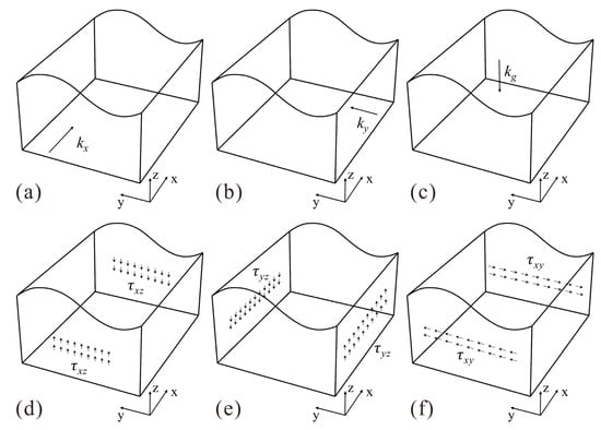
Figure 1. Different boundary conditions. (a) horizontal stress in the X-direction; (b) horizontal stress in the Y-direction; (c) gravity stress; (d) shear stress in the XZ-plane; (e) shear stress in the YZ-plane; and (f) shear stress in the XY-plane.

2.2. Optimization Solution Based on PSO-BP

2.2.1. Coordinate Transformation and Orthogonal Design

The in situ stress measurements are typically presented in the geodetic coordinate system. However, the inversion analysis for the in situ stress distribution in the underground cavern area is generally carried out in the computational coordinate system. Hence, before performing the inversion analysis, the stress state at the test points needs to be transformed from the geodetic coordinate system to the computational coordinate system, as demonstrated in Equation (1) [24].

$$\left.\begin{array}{l}{\sigma }_{\mathrm{x}}=L_1^2{\sigma }_1+L_2^2{\sigma }_2+L_3^2{\sigma }_3\\ {\sigma }_{\mathrm{y}}=M_1^2{\sigma }_1+M_2^2{\sigma }_2+M_3^2{\sigma }_3\\ {\sigma }_{\mathrm{z}}=N_1^2{\sigma }_1+N_2^2{\sigma }_2+N_3^2{\sigma }_3\\ {\tau }_{\mathrm{xy}}=L_1{M}_1{\sigma }_1+L_2{M}_2{\sigma }_2+L_3{M}_3{\sigma }_3\\ {\tau }_{\mathrm{yz}}=N_1{M}_1{\sigma }_1+N_2{M}_2{\sigma }_2+N_3{M}_3{\sigma }_3\\ {\tau }_{\mathrm{xz}}=L_1{N}_1{\sigma }_1+L_2{N}_2{\sigma }_2+L_3{N}_3{\sigma }_3\end{array}\right\}$$

(1)

where, $L_i=\mathrm{c}\mathrm{o}\mathrm{s}{\beta }_i\mathrm{c}\mathrm{o}\mathrm{s}{\alpha }_{ix}$, $M_i=\mathrm{c}\mathrm{o}\mathrm{s}{\beta }_i\mathrm{s}\mathrm{i}\mathrm{n}{\alpha }_{ix}$, $N_i=\mathrm{s}\mathrm{i}\mathrm{n}{\beta }_i$, ${\beta }_i$ is the angle between ${\sigma }_i$ and the horizontal plane, and ${\alpha }_{ix}$ is the angle between ${\sigma }_i$ and the direction of the x-axis.

In order to conduct in situ stress inversion using neural network intelligence algorithms, it is necessary to generate sufficient numerical data as input and output samples. The orthogonal design method is used to design the training sample scheme and thus calculate more comprehensive and representative combinations of boundary conditions at a lower computational cost. This method utilizes orthogonal design tables to effectively address the challenges posed by multi-factor design and optimal level determination. Table 1 shows a typical four-factor and three-level L9(3⁴) orthogonal design. The designed boundary condition scheme is then input into FLAC^3D software, respectively. The simulated stresses at the in situ stress test points, together with the boundary conditions, serve as the training samples for the network.

Table 1. Typical orthogonal design table L9(3⁴).

No.	A	B	C	D
1	A1	B1	C1	D1
2	A1	B2	C2	D2
3	A1	B3	C3	D3
4	A2	B1	C2	D3
5	A2	B2	C3	D1
6	A2	B3	C1	D2
7	A3	B1	C3	D2
8	A3	B2	C1	D3
9	A3	B3	C2	D1

2.2.2. PSO Optimized BP Network Algorithm

The fundamental principle of in situ stress inversion involves the establishment of a nonlinear relationship between the stress state and the model boundary conditions in order to identify the optimal boundary conditions that correspond with the measurement data. The BP neural network is widely used in underground engineering due to its capacity to deal with nonlinear problems [25,26]. However, the BP algorithm has some unavoidable limitations in addressing complex nonlinear problems. For example, many parameters should be initialized in the BP algorithm, such as weights, thresholds, error tolerance, etc. Some of these parameters that are determined empirically and roughly are sometimes not appropriate for a specific problem, and this limitation makes the BP algorithm quite unstable. Thus, in this paper, the PSO has been used to optimize the BP initial parameters to improve the stability and accuracy of the final result. The specific implementation steps of the PSO-BP intelligent optimization algorithm are as follows [21,27]:

(1) Determine the structure of the BP neural network.

(2) Encode the BP connection weights and thresholds; the particle dimension D is the sum of all weights in neural networks and is expressed as:

$$D=S_1\times R+S_1\times S_2+S_1+S_2$$

(2)

where, $R$, $S_1$, and $S_2$ are the numbers of neurons in the input, hidden, and output layers, respectively.

(3) Initialize the basic parameters of the particle swarm.

(4) Define the fitness function: the mean square error of BP is used as the function of fitness value, and the function is expressed as:

$$Fitness=\frac{1}{N}{\displaystyle {\sum }_{i=1}^N{\displaystyle {\sum }_{o=1}^{S_2}{(d_{io}(x_i)-y_{io})}^2}}$$

(3)

where N represents the total number of input samples, $d_{io}\left(x_i\right)$ is the o-th output result for the i-th group of input samples, and $y_{io}$ is the corresponding actual value.

(5) Based on the input-output sample pair, each particle’s fitness value is calculated using the forward algorithm and the fitness function of the BP network.

(6) For each particle, if $Fitness\left[i\right]$ is less than the $P_{best}$, let $P_{best}$ equal $Fitness\left[i\right]$; if $Fitness\left[i\right]$ is less than the $G_{best}$, let $G_{best}$ equal $Fitness\left[i\right]$;

(7) Update the velocity and position of the particles by Equations (4) and (5) and ensure that the particle velocity does not exceed the velocity limit ($v_{\max }$).

$$v_{ij}(t+1)=v_{ij}(t)+c_1{r}_1(t)\left[p_{ij}(t)-x_{ij}(t)\right]+c_2{r}_2(t)\left[p_{gj}(t)-x_{ij}(t)\right]$$

(4)

$$x_{ij}(t+1)=x_{ij}(t)+v_{ij}(t+1)$$

(5)

where x_ij and v_ij are the position and velocity of particles i in the j-th dimensional component, respectively; P_ij and P_gj are the individual extremum and global extremum of particles i in the j-th dimensional component, respectively; c₁ and c₁ are acceleration constants, which normally take the same value between 1.5 and 2.5; r₁ and r₂ are random numbers ranging from 0 to 1.

(8) Calculate the error of the PSO-BP algorithm as:

$$E=\frac{1}{t}{\displaystyle {\sum }_{i=1}^{t}J(G_{best}{}^{(i)})}$$

(6)

where $J(G_{best}{}^{(i)})$ is the fitness of the global optimal value in the i-th iteration and t is the current iteration time.

(9) If the error (E) is within the preset tolerance or the number of iterations reaches its maximum, the final solution is the vector of the global optimal position ($G_{best}$) in the last iteration. Otherwise, return to step 5.

2.2.3. PSO-BP Inversion Method

To enhance the accuracy of in situ stress inversion results, a nonlinear numerical analysis approach was proposed that combines the model boundary conditions with the PSO-BP algorithm. In this method, the complex geological movements are resolved into six basic boundary conditions, and then, through FLAC^3D software, the stress state of each boundary is calculated to form the network samples. The PSO-BP neural network is used to establish a nonlinear relationship between the boundary conditions and the stress state at specific testing locations. Finally, the optimal boundary conditions that coincide with the measurement results are obtained through iterative searching. The primary implementation steps are shown in Figure 2:

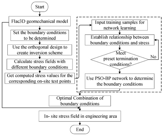
Figure 2. Flow chart of the PSO-BP in situ stress inversion method.

3. Application to the Shuangjiangkou Hydropower Station

3.1. Measured Results of In Situ Stress in Underground Cavern Zones

3.1.1. General Situation of Engineering Geology

The Shuangjiangkou hydropower station in Jinchuan County, Sichuan Province, is the fifth power station in the Dadu River basin. Figure 3 shows the site of the Shuangjiangkou hydropower station, which has the highest dam in the world. The underground cavern is deeply buried on the left bank with a horizontal depth of 300–500 m and a vertical depth of 42 m, and its axial azimuth is N10°W. F1 is the main fault distributed around the underground cavern area, which has a width of 0.5 to 0.6 m, and the occurrence is about N79°W/SW∠48°. A lamprophyre also occurred about N35°–50°W/SW∠72°–75° at the cavern area, with a width of 0.8–1 m. In general, the Shuangjiangkou underground cavern area mainly comprises porphyritic granite with different degrees of weathering. Currently, empirical systems, such as rock-mass rating (RMR), tunneling quality index (Q) system, and geological strength index (GSI), are mainly utilized in international rock engineering projects [28,29,30]. In the geological survey report of Shuangjiangkou Hydropower Station, the (basic quality index of rock mass) BQ method [31] is employed to classify the rock mass into four types of materials, namely, class II (fresh granite), class III (moderately weathered granite), class IV (strongly weathered granite), and class V (geological structures), as listed in Table 2.

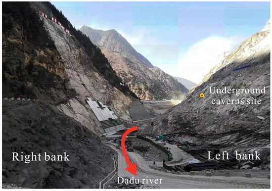
Figure 3. Dam site of Shuangjiangkou Hydropower Station.

Table 2. The mechanical parameters.

Type of Rock Mass	Rock Classification	Density (kg/m3)	Young’s Modulus E (GPa)	Poisson’s Ratio μ	Cohesion c (MPa)	Friction Coefficient f
Fresh granite	II	2600	32.9	0.25	1.5	1.3
Moderately weathered granite	III	2550	25.0	0.30	1.0	1.0
Strongly weathered granite	IV	2350	20.0	0.32	0.5	0.8
Geological structures	V	2300	6.0	0.35	0.1	0.35

3.1.2. Analysis of the Field Test

In situ stress measurements are a direct method for identifying the magnitude, direction, and distribution of in situ stress in the engineering field. Figure 4 displays the layout of in situ stress measurement points around the underground caverns on the left bank. The five measurement points are situated parallel to the main powerhouse’s axis and located inside the SPD9# structure at an elevation of 2268 m. The measured data is obtained in the geodetic coordinate system, and thus it is necessary to transform them into the model coordinate system using Equation (1). The transformed results are listed in Table 3.

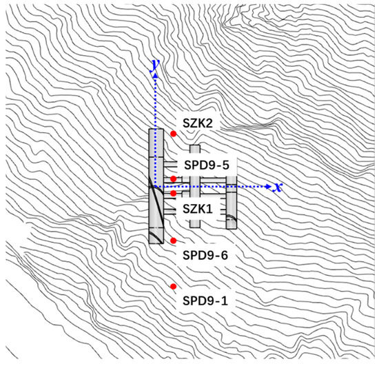
Figure 4. Distribution of in situ stress measured points.

Table 3. Stress components from in situ stress measurements around the underground caverns.

Test No.	Test Point	Burial Depth	σx/MPa	σy/MPa	σz/MPa	τxz/MPa	τyz/MPa	τxy/MPa
1#	SZK2	549 m	16.92	23.50	15.04	4.44	−3.19	1.54
2#	SPD9-5	470 m	19.26	22.74	16.66	0.33	−7.11	4.71
3#	SZK1	431 m	10.21	15.95	9.10	0.86	−2.60	−0.52
4#	SPD9-6	357 m	18.64	21.86	13.56	4.29	−2.47	6.81
5#	SPD9-1	308 m	15.84	22.18	24.01	1.64	−3.61	1.37

As shown in Table 3, the measured stress in the x-axis direction in the cavern area is 10.21–19.26 MPa, which is approximately 1.1 to 1.4 times greater than that in the vertical direction. Similarly, the stress in the horizontal y-axis direction ranges from 15.95 to 23.50 MPa, which is around 1.4 to 1.8 times greater than the vertical stress. The measured stress values are ranked as σ_y, σ_x, and σ_z in descending order, with horizontal stress σ_y and σ_x being higher than the vertical stress σ_z. This suggests that the tectonic movements have a significant impact on the stress distribution in the Shuangjiangkou underground cavern area. The shear stress values in the cavern area are generally low, with an average of 2.3 MPa for τ_xz, −3.7 MPa for τ_yz, and 2.8 MPa for τ_xy in the three directions.

The monitoring data used in the back analysis may directly affect the accuracy of the inversed in situ stress distribution, as it is the main input for the back analysis algorithm. Therefore, filtering the illogical measured points is necessary for the inversion process. As shown in Table 3, the stress values at the 3# measured point are smaller than the others, and considering that the 3# point is located near the F1 fault, the stress decreases in this region may be reasonable. Notably, despite the fact that the 5# point is located at the lowest burial depth of just 308 m compared to the highest 1# point of 549 m, the σ_z value at this point is about 24 MPa, ranking first among these five measurement points (the average value being 15.6 MPa). This means that there probably exist stress fluctuations near the 5# point area, and the measured data at this point may not properly reflect the overall in situ stress distribution in the engineering area. However, to consider the comprehensiveness and diversity of the input sample, all five measurement points were included in the inversion calculation.

3.2. Inversion Analysis of the In Situ Stress Distribution

3.2.1. Numerical Model

The inversion model should provide a comprehensive analysis of the impact of topography, geomorphology, lithology, and geological structures on the engineering field. After considering the precise locations of the testing points, a numerical model centered on the main powerhouse was established. As shown in Figure 5a, the 3D model can be mainly divided into three layers. The upper layer, represented by the color red, consists of strongly weathered granite. The middle layer, depicted in blue, is composed of moderately weathered granite. Finally, the lower layer, shown in green, comprises fresh rock. The geological structures, namely the F1 fault and lamprophyre, are simulated in the model through the fine mesh with specific thicknesses, as shown in Figure 5b. Besides, the spatial relationships between the F1 fault, lamprophyre, and underground caverns were determined based on a geological survey report. The underground cavern group of the Shuangjiangkou hydropower station consists of three parallel caverns (the main powerhouse, transformer chamber, and tailrace surge chamber) and some auxiliary caverns such as the penstock and generatrix tunnels. The range of the model requires an adequate length to minimize boundary effects and ensure an appropriate distance between the underground caverns and boundaries. The Flac^3D model has dimensions of 700 m in the x-axis (vertical axial direction), 700 m in the y-axis (axial direction), and 1100 m in the z-axis (elevation direction). The model has been extended to include the ground surface above the underground caverns, consisting of 477,685 nodes and 753,151 brick elements. The mesh is primarily composed of eight-node hexahedral elements, which exhibit uniform size and excellent morphology. Besides, to improve the computational accuracy, the mesh in the underground cavern area was further refined, with a minimum mesh density of 0.5m. In FLAC^3D software, the Mohr-Coulomb criterion is commonly used to model the behavior of rock under different loading conditions, which is the criterion utilized in this back analysis. The required mechanical parameters of all materials for this criterion, such as Young’s modulus, Poisson’s ratio, and strength parameters, are listed in Table 2, according to the geological survey report of Shuangjiangkou Hydropower Station.

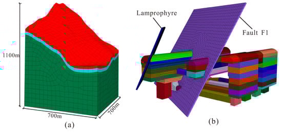
Figure 5. Numerical model for the in situ stress inversion. Mesh model of the surrounding mountain (a) and underground cavern and main geological structures (b).

3.2.2. Orthogonal Design Experiment

Obtaining accurate in situ stress distribution through neural networks requires a sufficient number of comprehensive training samples. Therefore, the in situ stress at the measurement points under different boundary conditions was generated through FLAC^3D software. The training sample scheme was established using an orthogonal design. Firstly, the six boundary condition coefficients of in situ stress inversion in FLAC^3D were determined according to the inversion theory in Section 2.1. Then, the test data in Table 3 was used as the base values for each parameter. The weight coefficient k_g was 1.3, the horizontal stress coefficients k_x and k_y were 1.3 and 1.6, respectively, and the shear stress coefficients were 2.3 MPa, −3.7 MPa, and 2.8 MPa, respectively. The weight coefficient, the horizontal stress structure coefficients, and the shear stress coefficients were varied within a range of 10%, 20%, and 30%, respectively, based on the base values. As shown in Table 4, an L49 (7⁶) orthogonal scheme was designed. The 49 sets of boundary condition schemes were then input into FLAC^3D software. The boundary conditions and the simulated in situ stress at the testing points constitute the training samples for the network.

Table 4. Boundary condition scheme L₄₉(7⁶).

Test No.	kg	kx	ky	τxz/MPa	τyz/MPa	τxy/MPa
1	0.91	0.91	1.12	1.61	−2.59	1.96
2	1.04	1.17	1.60	2.53	−4.44	3.64
3	1.17	1.43	2.08	1.84	−3.70	3.36
4	1.30	1.69	1.44	2.76	−2.96	3.08
5	1.43	1.04	1.92	2.07	−4.81	2.80
6	1.56	1.30	1.28	2.99	−4.07	2.52
7	1.69	1.56	1.76	2.30	−3.33	2.24
8	0.91	1.69	1.92	2.53	−3.70	2.52
9	1.04	1.04	1.28	1.84	−2.96	2.24
10	1.17	1.30	1.76	2.76	−4.81	1.96
11	1.30	1.56	1.12	2.07	−4.07	3.64
12	1.43	0.91	1.60	2.99	−3.33	3.36
13	1.56	1.17	2.08	2.30	−2.59	3.08
14	1.69	1.43	1.44	1.61	−4.44	2.80
15	0.91	1.56	1.60	1.84	−4.81	3.08
16	1.04	0.91	2.08	2.76	−4.07	2.80
17	1.17	1.17	1.44	2.07	−3.33	2.52
18	1.30	1.43	1.92	2.99	−2.59	2.24
19	1.43	1.69	1.28	2.30	−4.44	1.96
20	1.56	1.04	1.76	1.61	−3.70	3.64
21	1.69	1.30	1.12	2.53	−2.96	3.36
22	0.91	1.43	1.28	2.76	−3.33	3.64
23	1.04	1.69	1.76	2.07	−2.59	3.36
24	1.17	1.04	1.12	2.99	−4.44	3.08
25	1.30	1.30	1.60	2.30	−3.70	2.80
26	1.43	1.56	2.08	1.61	−2.96	2.52
27	1.56	0.91	1.44	2.53	−4.81	2.24
28	1.69	1.17	1.92	1.84	−4.07	1.96
29	0.91	1.30	2.08	2.07	−4.44	2.24
30	1.04	1.56	1.44	2.99	−3.70	1.96
31	1.17	0.91	1.92	2.30	−2.96	3.64
32	1.30	1.17	1.28	1.61	−4.81	3.36
33	1.43	1.43	1.76	2.53	−4.07	3.08
34	1.56	1.69	1.12	1.84	−3.33	2.80
35	1.69	1.04	1.60	2.76	−2.59	2.52
36	0.91	1.17	1.76	2.99	−2.96	2.80
37	1.04	1.43	1.12	2.30	−4.81	2.52
38	1.17	1.69	1.60	1.61	−4.07	2.24
39	1.30	1.04	2.08	2.53	−3.33	1.96
40	1.43	1.30	1.44	1.84	−2.59	3.64
41	1.56	1.56	1.92	2.76	−4.44	3.36
42	1.69	0.91	1.28	2.07	−3.70	3.08
43	0.91	1.04	1.44	2.30	−4.07	3.36
44	1.04	1.30	1.92	1.61	−3.33	3.08
45	1.17	1.56	1.28	2.53	−2.59	2.80
46	1.30	0.91	1.76	1.84	−4.44	2.52
47	1.43	1.17	1.12	2.76	−3.70	2.24
48	1.56	1.43	1.60	2.07	−2.96	1.96
49	1.69	1.69	2.08	2.99	−4.81	3.64

3.2.3. Identification of Boundary Conditions

A reliable nonlinear relationship between boundary conditions and the stress at the measured points is crucial for the accuracy of the inversed in situ stress distribution. However, the traditional method may encounter some issues such as ‘over-fitting’ or ‘under-fitting’ due to the uncertainty in the training sample size. The limitations restrict the ability of nonlinear mapping to approximate and subsequently affect the accuracy and reliability of the algorithm results. To address this issue, the PSO optimization method was used to optimize the BP neural network and establish a more accurate and reliable nonlinear model.

The PSO-BP neural network was trained using the boundary conditions listed in Table 4 as input samples and the corresponding calculated stresses at the measured points as sample outputs. The Shuangjiangkou hydropower station has five measurement points around the left underground caverns, each with six stress values; thus, a 30-16-6-6 topological network was constructed. The mean square error of the network model was set to 10⁻⁸, which was used to judge the training accuracy of iterations. The PSO-BP network was stopped after 3367 iterations when the error reached the preset value. Subsequently, the actual stresses at each measured point are input into the trained PSO-BP model to search for the optimal combination of boundary conditions. The inversed coefficients obtained by the PSO-BP neutral network are k_g = 1.43, k_x = 1.26, k_y = 1.60, τ_xz = 1.61 MPa, τ_yz = −2.51 MPa, and τ_x = 1.44 MPa.

To validate the accuracy of the determined boundary conditions, the obtained coefficients are utilized in the FLAC^3D software for additional forward analysis. Table 5 gives the stress results for each measurement point. It shows that the analysis results are generally acceptable for most points, except for the resulted σ_z of point 5#, where the analysis error is 20.33%. The average analysis error for the remaining points is 8.09%. Compared with Table 3, the measured σ_x and σ_y of point 5# are almost equal to those of other points, but the measured σ_z of point 5# is 7–15 MPa greater than that of other points, so it may not be accurately measured. As a result, the back-analysis σ_z of point 5# does not match very well with the measured data. Figure 6 compares the inversed and tested stresses. The dashed line indicates where the two stresses are equal. It can be observed that there is excellent agreement between the PSO-BP results and measured data, with a correlation coefficient of about 0.95.

Table 5. Computational stress components at test points.

Test No.	σx/MPa	σy/MPa	σz/MPa	τxz/MPa	τyz/MPa	τxy/MPa
1	18.33	20.07	14.83	1.02	−2.63	1.22
2	18.08	20.91	14.45	1.12	−2.18	1.27
3	11.98	18.10	9.41	1.63	−0.80	0.37
4	17.72	22.48	14.02	1.69	−2.34	0.73
5	17.96	23.49	14.00	2.65	−2.45	0.79

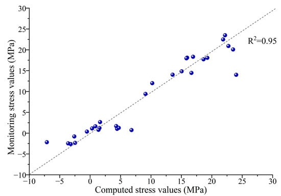
Figure 6. Comparison of inverted results with measured results.

3.3. Characteristics of In Situ Stress around Underground Caverns

The purpose of the in situ stress inversion is to investigate the distribution of in situ stress in the engineering area. By studying its distribution characteristics, it is possible to provide some references for the engineering’s design, construction, and long-term stability. Hence, based on the boundary conditions obtained from the PSO-BP inversion, the distribution characteristics of the in situ stress in the Shuangjiangkou underground cavern area were computed.

Figure 7 shows the stress distribution in the cross-section of the main powerhouse, while Figure 8 plots that in the longitudinal section direction. As can be seen, there is an increasing trend in the distribution of in situ stresses with the increase in rock burial depth. The shallow surface presents local stress relaxation with relatively low stress values in this area. This is followed by a stress transition zone, where the principal stress distribution gradually becomes horizontal with a progressive increase in stress. The deeper part of the rock has a higher stress level and a more stable stress state. The first principal stress ranges from 20 to 26 MPa, with some stress concentration occurring around the river valley. The third principal stress ranges from 14 to 18 MPa and is predominantly oriented in the vertical direction. Fault F1 and the lamprophyre notably influence the stress distribution in the main powerhouse area, resulting in a significant reduction in the stresses within 10 m.

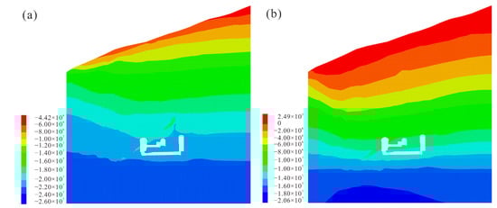
Figure 7. Stress distribution in the cross-section of the main powerhouse. (a) the first principal stress, (b) the third principal stress.

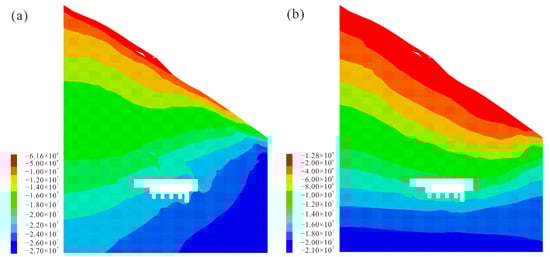
Figure 8. Stress distribution in the longitudinal section of the main powerhouse. (a) the first principal stress; and (b) the third principal stress.

The results of the in situ stress inversion indicate that weak structural planes may have the potential to significantly influence the stress state of an engineering area. As shown in Figure 9, all three stress components increase with the buried depth while remaining relatively consistent within the main powerhouse area at the same elevation. There is a sudden drop in stress values at the fault area, with the σ_x falling to around 10–12 MPa, σ_y about 17–20 MPa, and σ_z about 8–10 MPa. However, the stress state around the tailrace surge chambers does not fluctuate since the fault and the lamprophyre do not intersect with the tailrace surge chambers. Thus, faults and lamprophyre could notably influence the in situ stress distribution, leading to a reduction in the in situ stress value of the surrounding rock.

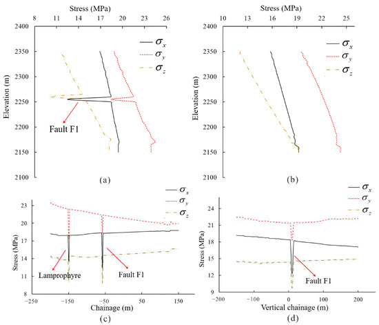
Figure 9. Stress variations along the depth (a) in the main powerhouse and (b) in the tailrace surge chambers; Stress variations in the plane of 2260 m elevation along the axis of the main powerhouse (c) and along the vertical axis of the main powerhouse (d).

4. Discussion

To validate the improvement of the proposed method, a comparison between the PSO-BP in situ stress numerical analysis method and the conventional method is conducted in Shuangjiangkou Hydropower Station engineering.

For comparison, the BP network was constructed the same as the PSO-BP network in this study, with a topology of 30-16-6-6 and the mean square error of the network model set to 10⁻⁸. The BP neural network was also trained using the boundary conditions listed in Table 4 as input samples and the calculated stresses at the measured points as sample outputs. After the iterative search, the optimal combination of boundary conditions from the BP network method can be obtained. The inversed coefficients are k_g = 1.35, k_x = 1.18, k_y = 1.72, τ_xz = 0.73 MPa, τ_yz = −2.29 MPa, and τ_x = 1.75 MPa. Then, the obtained coefficients are utilized in the FLAC^3D software for additional forward analysis, which generates the computational results from the conventional method, as shown in Table 6. For comparison, the measured data and the results from the PSO-BP method are also listed in this table.

Table 6. Computational stress components at test points. A comparison of the computational stress of the two back analysis methods.

Test No.	Algorithm	σx/MPa	σy/MPa	σz/MPa	τxz/MPa	τyz/MPa	τxy/MPa
1	Measured	16.92	23.50	15.04	4.44	−3.19	1.54
	BP	14.50	21.07	13.47	0.69	−2.18	1.29
	PSO-BP	18.33	20.07	14.83	1.02	−2.63	1.22
2	Measured	19.26	22.74	16.66	0.33	−7.11	4.71
	BP	14.36	21.87	13.31	0.47	−1.88	1.45
	PSO-BP	18.08	20.91	14.45	1.12	−2.18	1.27
3	Measured	10.21	15.95	9.10	0.86	−2.60	-0.52
	BP	10.52	19.21	8.75	1.21	−0.21	0.71
	PSO-BP	11.98	18.10	9.41	1.63	−0.80	0.37
4	Measured	18.64	21.86	13.56	4.29	−2.47	6.81
	BP	14.22	23.49	13.21	1.30	−1.92	1.82
	PSO-BP	17.72	22.48	14.02	1.69	−2.34	0.73
5	Measured	15.84	22.18	24.01	1.64	−3.61	1.37
	BP	14.27	24.38	13.33	1.61	−2.07	0.95
	PSO-BP	17.96	23.49	14.00	2.65	−2.45	0.79

As can be seen, the BP network method also inversed a relatively reasonable combination of boundary conditions, while the average relative error of the PSO-BP results is 3.45% lower than that of the conventional method, indicating a closer approximation to the actual in situ stress. Therefore, for in situ stress inversion using the same engineering, the PSO-BP method may evidently improve the accuracy of the inversion results compared with the conventional BP network method. It should be noted that the PSO-BP method has some limitations, one of them being the requirement of sufficient input samples. While the huge training samples result in a significant increase in computational cost, the accuracy of the results may improve as the number of samples increases. Hence, it is necessary to select a reasonable and sufficient number of training samples for different engineering problems.

5. Conclusions

To improve the accuracy of the in situ stress inversion, a PSO-BP in situ stress numerical analysis method was proposed and applied to the in situ stress inversion of the Shuangjiangkou Hydropower Station underground engineering. Based on the results of the numerical simulation, the feasibility of the method was verified, and the characteristics of the in situ stress distribution around the underground caverns were obtained. The main conclusions are drawn as follows:

(1)

The complex geological movements can be decomposed into six basic boundary conditions for numerical simulation, and the PSO-BP neural network can then identify the optimal boundary conditions that best represent the measured in situ stresses.

(2)

The average relative error of the inversion results obtained by the proposed method is 3.45% lower than those obtained by the traditional method; thus, the proposed method is more effective and the inversed in situ stress distribution is more reasonable.

(3)

The distribution of in situ stresses increases as the buried depth of rock increases. The first principal stress ranges from 20 to 26 MPa, with stress concentration around the river valley. The third principal stress ranges from 14 to 18 MPa and is oriented approximately vertically.

(4)

Fault F1 and the lamprophyre notably influence the stress distribution in the main powerhouse area, with 15–30% localized stress reduction in the rock mass within 10m, which may provide a reference for similar engineering with weak structural planes.

References

- Song, Z.F.; Sun, Y.J.; Lin, X. Research on In Situ Stress Measurement and Inversion, and its Influence on Roadway Layout in Coal Mine with Thick Coal Seam and Large Mining Height. Geotech. Geol. Eng. 2017, 36, 1907–1917. [Google Scholar] [CrossRef]
- Li, S.; Feng, X.T.; Li, Z.H.; Chen, B.; Zhang, C.; Zhou, H. In situ monitoring of rockburst nucleation and evolution in the deeply buried tunnels of Jinping II hydropower station. Eng. Geol. 2012, 137–138, 85–96. [Google Scholar] [CrossRef]
- Zhang, G.; Li, Y.; Meng, X.; Tao, G.; Wang, L.; Guo, H.; Zhu, C.; Zuo, H.; Qu, Z. Distribution Law of In Situ Stress and Its Engineering Application in Rock Burst Control in Juye Mining Area. Energies 2022, 15, 1267. [Google Scholar] [CrossRef]
- Gong, M.; Qi, S.; Liu, J. Engineering geological problems related to high geo-stresses at the Jinping I Hydropower Station, Southwest China. Bull. Eng. Geol. Environ. 2010, 69, 373–380. [Google Scholar] [CrossRef]
- Haimson, B.C. Deep in-situ stress measurements by hydrofracturing. Tectonophysics 1975, 29, 41–47. [Google Scholar] [CrossRef]
- Aadnoy, B.S. Inversion technique to determine the in-situ stress field from fracturing data. J. Pet. Sci. Eng. 1990, 4, 127–141. [Google Scholar] [CrossRef]
- Ljunggren, C.; Chang, Y.; Janson, T.; Christiansson, R. An overview of rock stress measurement methods. Int. J. Rock Mech. Min. Sci. 2003, 40, 975–989. [Google Scholar] [CrossRef]
- Bao, T.; Burghardt, J. A Bayesian Approach for In-Situ Stress Prediction and Uncertainty Quantification for Subsurface Engineering. Rock Mech. Rock Eng. 2022, 55, 4531–4548. [Google Scholar] [CrossRef]
- Meng, Q.; Chen, Y.; Zhang, M.; Han, L.; Pu, H.; Liu, J. On the Kaiser Effect of Rock under Cyclic Loading and Unloading Conditions: Insights from Acoustic Emission Monitoring. Energies 2019, 12, 3255. [Google Scholar] [CrossRef]
- Xu, D.; Huang, X.; Jiang, Q.; Li, S.; Zheng, H.; Qiu, S.; Xu, H.; Li, Y.; Li, Z.; Ma, X. Estimation of the three-dimensional in situ stress field around a large deep underground cavern group near a valley. J. Rock Mech. Geotech. Eng. 2021, 13, 529–544. [Google Scholar] [CrossRef]
- Wang, B.L.; Ma, Q.C. Boundary element analysis methods for ground stress field of rock masses. Comput. Geotech. 1986, 2, 261–274. [Google Scholar] [CrossRef]
- McKinnon, S.D. Analysis of stress measurements using a numerical model methodology. Int. J. Rock Mech. Min. Sci. 2001, 38, 699–709. [Google Scholar] [CrossRef]
- Meng, W.; He, C. Back Analysis of the Initial Geo-Stress Field of Rock Masses in High Geo-Temperature and High Geo-Stress. Energies 2020, 13, 363. [Google Scholar] [CrossRef]
- Zhang, Z.; Gong, R.; Zhang, H.; Lan, Q.; Tang, X. Initial ground stress field regression analysis and application in an extra-long tunnel in the western mountainous area of China. Bull. Eng. Geol. Environ. 2021, 80, 4603–4619. [Google Scholar] [CrossRef]
- Chen, B.; Ren, Q.; Wang, F.; Zhao, Y.; Liu, C. Inversion Analysis of In-situ Stress Field in Tunnel Fault Zone Considering High Geothermal. Geotech. Geol. Eng. 2021, 39, 5007–5019. [Google Scholar] [CrossRef]
- Yu, R.; Tan, Z.; Gao, J.; Wang, X.; Zhao, J. Inversion and Analysis of the Initial Ground Stress Field of the Deep-Buried Tunnel Area. Appl. Sci. 2022, 12, 8986. [Google Scholar] [CrossRef]
- Yong, L.; Yunhua, G.; Weishen, Z.; Shucai, L.; Hao, Z. A modified initial in-situ Stress Inversion Method based onFLAC3D with an engineering application. Open Geosci. 2015, 7, 824–835. [Google Scholar] [CrossRef]
- Zhang, S.; Yin, S. Determination of in situ stresses and elastic parameters from hydraulic fracturing tests by geomechanics modeling and soft computing. J. Pet. Sci. Eng. 2014, 124, 484–492. [Google Scholar] [CrossRef]
- Li, X.; Zhou, X.; Xu, Z.; Feng, T.; Wang, D.; Deng, J.; Zhang, G.; Li, C.; Feng, G.; Zhang, R.; et al. Inversion Method of Initial In Situ Stress Field Based on BP Neural Network and Applying Loads to Unit Body. Adv. Civ. Eng. 2020, 2020, 15. [Google Scholar] [CrossRef]
- Li, G.; Hu, Y.; Li, Q.B.; Yin, T.; Miao, J.X.; Yao, M. Inversion Method of In-situ Stress and Rock Damage Characteristics in Dam Site Using Neural Network and Numerical Simulation—A Case Study. IEEE Access 2020, 8, 46701–46712. [Google Scholar] [CrossRef]
- Eberhart, R.; Kennedy, J. A new optimizer using particle swarm theory. In Proceedings of the Sixth International Symposium on Micro Machine and Human Science (Cat. No.95TH8079), MHS’95, Nagoya, Japan, 4–6 October 1995; pp. 39–43. [Google Scholar] [CrossRef]
- Guo, M.W.; Yin, S.D.; Li, C.G.; Wang, S.L. 3D In Situ Stress Estimation by Inverse Analysis of Tectonic Strains. Appl. Sci. 2021, 11, 5284. [Google Scholar] [CrossRef]
- Matsuki, K.; Nakama, S.; Sato, T. Estimation of regional stress by FEM for a heterogeneous rock mass with a large fault. Int. J. Rock Mech. Min. Sci. 2009, 46, 31–50. [Google Scholar] [CrossRef]
- Pielke, R.A. Chapter 6—Coordinate Transformations. In International Geophysics; Pielke, R.A., Ed.; Academic Press: Cambridge, MA, USA, 2013; Volume 98, pp. 111–141. [Google Scholar]
- Baghbani, A.; Choudhury, T.; Costa, S.; Reiner, J. Application of artificial intelligence in geotechnical engineering: A state-of-the-art review. Earth-Sci. Rev. 2022, 228, 26. [Google Scholar] [CrossRef]
- Jiang, Q.; Feng, X.T. Intelligent Stability Design of Large Underground Hydraulic Caverns: Chinese Method and Practice. Energies 2011, 4, 1542–1562. [Google Scholar] [CrossRef]
- Yuhui, S.; Eberhart, R.C. Parameter selection in particle swarm optimization. In Proceedings of the 7th International Conference, EP98, San Diego, CA, USA, 25–27 March 1998; pp. 591–600. [Google Scholar] [CrossRef]
- Bieniawski, Z.T. Engineering Rock Mass Classifications: A Complete Manual for Engineers and Geologists in Mining, Civil, and Petroleum Engineering; Wiley: Hoboken, NJ, USA, 1989. [Google Scholar]
- Rehman, H.; Ali, W.; Naji, A.; Kim, J.-j.; Abdullah, R.; Yoo, H.-K. Review of Rock-Mass Rating and Tunneling Quality Index Systems for Tunnel Design: Development, Refinement, Application and Limitation. Appl. Sci. 2018, 8, 1250. [Google Scholar] [CrossRef]
- Cai, M.; Kaiser, P.K.; Uno, H.; Tasaka, Y.; Minami, M. Estimation of rock mass deformation modulus and strength of jointed hard rock masses using the GSI system. Int. J. Rock Mech. Min. Sci. 2004, 41, 3–19. [Google Scholar] [CrossRef]
- The Ministry of Water Resources of China. Chinese National Standard GB/T 50218-2014: Standard for Engineering Classi-fication of Rock Mass; China Planning Press: Beijing, China, 2014.
Disclaimer/Publisher’s Note: The statements, opinions and data contained in all publications are solely those of the individual author(s) and contributor(s) and not of MDPI and/or the editor(s). MDPI and/or the editor(s) disclaim responsibility for any injury to people or property resulting from any ideas, methods, instructions or products referred to in the content. |
© 2023 by the authors. Licensee MDPI, Basel, Switzerland. This article is an open access article distributed under the terms and conditions of the Creative Commons Attribution (CC BY) license (https://creativecommons.org/licenses/by/4.0/).