Abstract
The finite element method (FEM) and the limit equilibrium method (LEM) are commonly used for calculating slope failure risk. However, the FEM needs to carry out post-processing to estimate slope sliding surface, while the LEM requires assumption of the shape and location of the sliding surface in advance. In this paper, an element failure risk method (EFR) for calculating soil slope failure risk is proposed based on element failure probability (EFP) acquired by plastic limit analysis. The proposed method does not require any assumptions about failure modes. Firstly, the non-common-node triangle element is used to discrete the slope then the random field is generated based on the Cholesky decomposition midpoint method. According to the reliability stochastic programming model and solution strategy, the external overload coefficient, bulk overload coefficient, slope stability coefficient and velocity field of the slope under each random field are obtained, according to which the failure of the element is judged and the failure risk of the slope is calculated. In order to verify the correctness of the proposed method, two classical slopes are systematically analyzed. The research shows that compared with the traditional slope failure risk analysis method, the greatest advantage of the proposed method is that it can capture all failure modes of the slope and greatly simplify the calculation of the slope failure consequences of each failure mode. An efficient upper bound method (UBM) parallel program is prepared, which greatly improves the calculation efficiency.
1. Introduction
The instability of slope can not only endanger people’s lives and property but also lead to great loss of national economy [1,2,3]. Under the long-term geological effects of deforestation, deposition and post-deposition, the shear strength parameters of slope soil mass show spatial variability. Research shows that the spatial variability of soil parameters is a major source of uncertainty in slope engineering. It not only affects bearing capacity and safety performance, but also has a significant influence on the slope failure mode [4,5,6]. Different failure modes correspond to different failure consequences. The traditional integrated failure probability (IFP) method based on the slope stability coefficient for failure risk analysis needs to count the failure modes individually. In addition, the calculation of the slope stability coefficient involves complex processes such as limit state definition and strength reduction. Therefore, it is urgent to develop new methods for slope failure risk analysis.
At present, the three most commonly used methods for slope stability analysis are the rigid body limit equilibrium method (LEM) [7,8,9], the finite element method (FEM) [10,11,12] and the limit analysis method (LAM) [13,14,15,16,17,18,19]. The LEM first assumes the sliding surface, then divides the soil on the sliding surface into strips and turns a hyper-static problem into a static problem by assuming the magnitude and direction of the inter-strip force. Based on different assumptions, a variety of LEMs have been formed, such as the Ordinary/Fellenius method, the Bishop Simplified method, the Morgenstern-Price method and the Spencer method. The LEM is widely used in engineering because of its clear concept and simple calculation. However, it possesses the following drawbacks when using this method for slope stability analysis considering spatial variability of parameters: (1) only considering the spatial variability of soil material in one dimension on the sliding surface, ignoring the influence outside the sliding surface [20]. Due to the deficiencies of LEM, the stress-strain relationship of soil cannot be accurately obtained [18,20]. Based on the principle of minimum potential energy, the FEM turns differential equations into linear algebraic equations to solve and simultaneously satisfies the constraints of equilibrium equations, geometric equations and constitutive relations of discrete triangular elements. LAM applies the upper and lower limit theorems generally observed by an ideal elastoplastic body and obtains the upper and lower limit solutions when the slope is in the limit state by constructing kinematically-admissible velocity fields and static admissible stress fields. It is known from the upper and lower limit theorems that the true solution must lie between the upper and lower limit solutions. This method can efficiently and accurately obtain the ultimate load [18,19], stability coefficient [13,14,15,16,17,18] and failure mode [5,18] of a slope in the limit state without considering the complex constitutive relationship of rock and soil mass. Zhang Xiaoyan et al. [18] and Li Liang et al. [19] set the shear strength parameters of soil as random variables and solved the upper and lower limit solutions. Li Ze et al. [21] studied the failure probability of slopes under the action of random groundwater levels from the perspective of element failure probability (EFP). Chen Chaohui et al. [20] found that the spatial variability of soil shear strength parameters has a significant influence on the slope failure mode. The above studies mostly focus on the slope failure probability and pay less attention to the failure consequences, which is not necessarily. For example, when a slope with multi-failure modes fails, different failure modes (shallow landslide/deep landslide) correspond to different failure consequence coefficients (sliding mass volume). The probability of a shallow landslide on a slope may be higher than that of deep landslide, but the failure consequence coefficient of a shallow landslide is smaller. In order to comprehensively consider the impact of slope failure probability (Pf) and the failure consequence coefficient (C), researchers put forward the concept of slope failure risk and defined it as the product of Pf and C [22,23,24,25]. However, whether based on LEM or FEM, it is necessary to first identify and count all failure modes. With large samples, the calculation efficiency is low. It is worth mentioning that Zhang Xiaoyan et al. put forward a slope reliability analysis method based on EFP in the document [18], which uses the slope stability coefficient and velocity field to calculate the EFP, providing a new idea for slope failure risk analysis. However, based on strength reduction, the dichotomy method is used to calculate the slope stability coefficient and judges whether the slope is in the limit state according to the external force overload coefficient; therefore, repeated reduction and judgment are difficult to avoid. In view of this, this paper combines the finite element discretization technique, the related non-Gaussian stochastic field simulation method, the upper bound method theory and stochastic planning theory to propose a new method for slope failure risk assessment base on EFP.
2. Methodologies
2.1. Limit State Function of Slope
There are usually two ways to cause a slope to reach the limit state. One is to gradually increase the external load, that is, the external force overload. The force can be distributed across the load and concentrated on the boundary; another is to gradually reduce the shear strength parameters of rock and soil materials, that is, strength reduction. The former defines the external force overload coefficient and the latter defines the strength reserve coefficient (stability coefficient). Therefore, the limit state function of a slope is:
where: = the limit state function obtained by gradually increasing the external load of the slope; = the limit state function obtained by gradually increasing the slope load; = the limit state function obtained by gradually reducing the shear strength parameters of soil materials; = the external load when the slope is in the limit state; = the external force overload coefficient of the slope; = the actual load of the slope; = the bulk density when the slope is in the limit state; = the bulk density overload coefficient of the slope; = the actual bulk density of the slope; = the strength reserve coefficient of the slope; , = cohesion and internal friction angle before strength reduction; , = cohesion and internal friction angle after strength reduction.
2.2. Stochastic Programming Model for Slope Failure Risk
Combining the advantages of FEM and LAM, the finite element limit analysis method can simulate complex geotechnical problems such as rainfall, earthquake, water level rise and fall, parameter spatial variability, etc. [6,20,26,27]. The UBM is mainly used to obtain the upper bound solution when the slope is in the limit state by constructing the kinematically admissible velocity field. Similar to the method in literature [16], the non-common-node triangular element is used to discretize the slope. When the spatial variability of soil parameters is considered, the triangular elements a and b have both mutual and self-correlation. The exponential autocorrelation function can be expressed as [28,29,30,31,32]:
where , = the horizontal and vertical coordinates of element a respectively; , = the horizontal and vertical coordinates of element b respectively; , = the fluctuation ranges in the horizontal and vertical coordinate directions respectively [28].
Taking into account the non-Gaussian distribution and mutual correlation of soil shear strength parameters, the relevant non-Gaussian field generation process is involved. In this paper, the Cholesky decomposition midpoint method is used to generate the random field. The specific expression is:
where: = the shear strength parameter of soil mass, ; = correlated non-Gaussian random fields; = correlated standard Gaussian random fields; , ; = the mean value of lognormal distribution of ; = the standard deviation of lognormal distribution of ; = the mean value of the corresponding normal variable of ; = the standard deviation of the corresponding normal variable of .
Non-common-node triangular elements are used to construct the kinematically-admissible velocity field that simultaneously satisfies the plastic flow conditions of the triangular elements, the plastic flow conditions of discontinuous and the velocity boundary conditions of the triangular elements. It can be understood from the upper limit theorem that the external load corresponding to the kinematically-admissible velocity field is the ultimate upper limit load of the slope, so the UBM can be considered as a stochastic programming problem for solving the minimum value, and the velocity of the triangle element node is decision variable. Based on the previous studies, the slope reliability analysis model of gradually increasing the distributed load on the boundary to cause the slope to reach the limit state is:
The slope reliability analysis model that uses bulk density overload to cause the slope to reach the limit state is:
where: = the internal power of finite elements; = the internal power of the velocity discontinuities; = the external work power done by the external load or dead weight on the velocity of the finite element nodes; = the plastic multiplier; = the decision variable; , = the matrix of plastic flow constraint conditions of the finite element e; , = the matrix of plastic flow constraint conditions of the velocity discontinuity d; = the coordinate transformation matrix of the finite element b on the boundary; = the velocity vector of finite element e, , = the quantity of finite element; = the velocity vector of the velocity discontinuity d, , = the quantity of velocity discontinuity; = the velocity vector of the boundary finite element b, , = the quantity of the finite elements on the boundary. The meanings of other related expressions are detailed in the literature [16].
2.3. Solution Strategy of Stochastic Programming Model
In Equations (5) and (6), , , and are all related to soil shear strength parameters. For such problems, based on a Monte Carlo simulation (MCS), an iterative method was proposed to solve them by LI Ze et al. [21] and Peng Pu et al. [5]. The specific steps are as follows:
(1) Determine the geometric dimensions of the slope and the information and distribution characteristics of the soil shear strength parameters;
(2) Non-common node triangular elements are used to discretize the soil slope;
(3) According to the position of finite elements and the distribution characteristics of soil shear strength parameters, based on the midpoint method of Cholesky decomposition the random field is generated thusly:
where: = the cohesion of the triangular element e in the th non-Gaussian random field; = the internal friction angle of the triangular element e in the th non-Gaussian random field; = the cohesion of the triangular element e in the th standard Gaussian random field; = the internal friction angle of the triangular element e in the standard Gaussian random field; , ; ; ; = the mean value of cohesion with lognormal distribution; = the mean value of the internal friction angle with lognormal distribution; = the standard deviation of cohesion with lognormal distribution; = the standard deviation of the internal friction angle with lognormal distribution; = the mean value of normal variables of ; = the mean value of normal variables of ; = the standard deviation value of normal variables of ; = the standard deviation value of normal variables of ; = the quantity of cohesion and internal friction angle of random fields of soil material where and = pore water pressures at the three nodes of the finite element e, respectively. The meanings of other related expressions are detailed in the literature [25].
(4) Nested from to , substitutethe soil shear strength parameters random field in group into the UBM linear programming model Equation (5) or Equation (6), which are solved by using the dual simplex optimization algorithm in order to obtain the random numbers of external force overload coefficients or bulk density overload coefficients . Meanwhile, use the dichotomous iterative to solve the random numbers of the stability coefficients and the kinematically-admissible velocity field.
(5) Calculate the statistical reliability index of the slope. The numerical solution flow chart is shown in Figure 1.
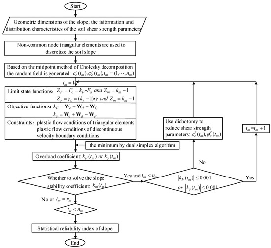
Figure 1.
Flow chart of a numerical solution using UBM for a slope.
2.4. Element Failure Probability of Slope
Traditional slope reliability analysis generally adopts the integrated failure probability method [33] and uses the threshold value of slope stability coefficient for evaluation. It is considered that when the slope stability coefficient , then the slope remains stable; when the slope stability coefficient , then the slope becomes unstable. Therefore, the slope failure function based on the IFP of km is expressed as:
Further, according to the concept of slope in a limited state, it can be determined that if the slope has been destroyed without applying any external load or applying any opposite direction load, then the external overload coefficient and bulk density overload coefficient are both less than 0. Therefore, the slope-failure function based on the IFP of kF can be expressed as:
The slope failure function based on IFP of kγ can be expressed as:
The IFP of a slope is expressed as:
where = the failure probability of the slope, of which .
Therefore, the equation calculation for slope failure risk (IPF-FR) based on the IFP [25] is:
where = the failure risk of the slope; = the failure probability of the slope; = the failure risk coefficient.
Equation (10) is widely used in slope failure risk analysis, but the impact of multi-failure modes of slopes is not considered. In view of this, Huang et al. [34] proposed a slope failure risk equation based on multi-failure modes, in which the failure risk of the k-th failure mode is:
where = the failure risk of the k-th failure mode; = the failure probability of the k-th failure mode; = the failure risk coefficient of the k-th failure mode, where k = 1,2,..., Nf, Nf is the quantity of failure modes.
The failure risk of a slope is:
where = the slope failure risk by M-IFP.
Compared with Equation (12), Equation (14) can calculate the slope risk assessment of single failure mode and multi-failure modes at the same time. However, both LEM and FEM must be used to conduct screening of complex failure modes in advance. It is worth mentioning that Zhang Xiaoyan et al. [18] proposed the concept of element failure probability based on the slope stability coefficient (km-uc-EFP), which uses the slope stability coefficient obtained by solving the mathematical programming model of the UBM and the failure condition of slope elements determined by a kinematically-admissible velocity field to obtain the failure condition of each area. The failure function is:
where = the failure function of the element e in the th random field; = the velocity of the element in the th random field.
In this paper, two new concepts of EFP based on the external overload coefficient (kF-uc-EFP) and based on the bulk density overload coefficient (kγ-uc-EFP) are proposed for the first time. According to the concept of slope in the limit state, it can be determined that if the slope has been destroyed without applying any external load or applying any opposite direction load, then the external overload coefficient and bulk density overload coefficient are both less than 0. In addition, when plastic flow occurs in the discrete triangular element, the relative velocity of the element will be generated compared with that of the fixed element on the boundary; that is, the velocity at the centroid of the element is greater than 0, which is the failure element. Therefore, the slope failure function based on kF-uc-EFP is expressed as:
The slope failure function based on kγ-uc-EFP can be expressed as:
The EFP of the slope can be unified as:
where = the failure probability of slope element e, of which .
The failure risk of the slope element can be expressed as:
where = the failure risk of slope element e; = the failure risk coefficient of slope element e, .
Further the failure risk of a slope is:
where = slope failure risk by M-uc-EFP.
The mean and standard deviation of the external overload coefficient , bulk density overload coefficient and slope stability coefficient can be obtained by statistics. Specifically, they are:
where , = the mean value and standard deviation of M; ; .
3. Calibration and Application
Based on the solution strategy of the slope failure risk model, the UBM parallel calculation program was created in Python. Two classical slopes are analyzed and compared with FEM and LEM to verify the effectiveness and correctness of the proposed method.
3.1. Case 1: A Homogeneous Slope
3.1.1. Homogeneous Slope Description
Figure 2 shows a slope with a height of 10 m, a top width of 10 m and a slope ratio of 1:1. Many scholars have calculated and analyzed this slope [5,28,35]; however, most studies only focus on the slope failure probability and there is no systematic analysis or research on the ultimate bearing capacity and slope failure risk. For this reason, the ultimate bearing capacity and slope failure risk are researched based on the proposed method. Using non-common-node finite elements discrete to the slope, 1360 finite elements, 4080 non-common nodes and 2099 discontinuities are obtained. The soil capacity γ is set to a constant value of 20.0 kN/m3 and other calculation parameters are shown in Table 1. The quantity of random fields is nm = 1000, and Equation (7) was used to obtain the 1000 random fields.
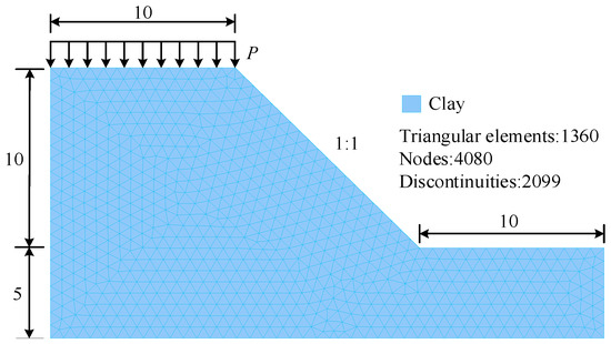
Figure 2.
Homogeneous slope calculation model.

Table 1.
Calculation parameters of the slope.
3.1.2. Result of Homogeneous Slope
The slope is calculated by running the UBM parallel calculation program on a small work station (processor: AMD Ryzen 3970X, 32 cores, physical memory: 128 GB). Table 2 lists the results obtained by the FEM, LEM and UBM. Figure 3 and Figure 4 give the relationship between top load, bulk density and the stability slope coefficient when . Figure 5 gives the histogram of the external overload coefficient , bulk overload coefficient and slope stability coefficient .
Table 2.
Homogeneous slope reliability results of different methods.
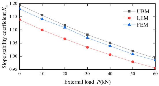
Figure 3.
Relationship between external load and slope stability coefficient of homogeneous slope.
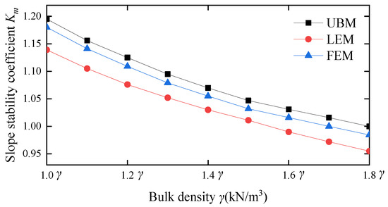
Figure 4.
Relationship between bulk density and slope stability coefficient of homogeneous slope.
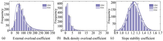
Figure 5.
Histogram of , and of homogeneous slope.
The calculation results show that:
- (1)
- The slope reliability results of different methods are compared in Table 2. It can be seen that the mean values of the external overload coefficient, bulk density overload coefficient and slope stability coefficient obtained by the UBM are all greater than the calculated results obtained by the LEM and FEM, but the errors are small. From the upper limit theorem, it is clear that the external load corresponding to the kinematically-admissible velocity field obtained by the UBM is the strict upper bound of the ultimate load; that is, the , and obtained by the UBM must be greater than the actual solution. Therefore, when the UBM is used to calculate the slope failure probability, it will be slightly underestimated. However, compared with the traditional LEM, the UBM can fully determine the random field of two-dimensional soil slope shear strength parameters. It is unnecessary to assume the critical sliding surface in advance and it is also unnecessary to convert the super-static problem into the static problem by assuming the magnitude and direction of the inter-slice force. Compared with FEM, the UBM can ignore the complex constitutive relationship of rock and soil mass. The slope complex problem is solved according to the plastic flow constraint of triangular elements, the plastic flow constraint of discontinuities and the velocity boundary condition of triangular elements which must be met simultaneously when the slope is in the limit state and therefore the calculation efficiency is more efficient.
- (2)
- Based on the , and , the slope failure probability can be calculated, which is close or equal. From the perspective of calculation efficiency, the above three methods in this paper can carry out large-scale parallel calculation. However, it required 0.52 h (about 20.8 h for single thread calculation), 0.53 h (about 21.2 h for single thread calculation) and 4.16 h (about 166.4 h for single thread calculation), respectively, to calculate the , and of 1000 random field samples. It required 28.4, 29.1 and 127.2 h, respectively, to calculate the , and using the FEM method for the same sample. It is clear that the calculation efficiency of slope reliability analysis based on and is much higher than that . The main reason is that solving the requires repeated calculation of or and judging whether the slope is in the limit state, as shown in Figure 1, and therefore the calculation efficiency is low.
- (3)
- Figure 3 and Figure 4 reflect the process of gradually increasing the top load and bulk density to cause the slope to reach the limit state. It can be observed intuitively that with the gradual increase of top load P and bulk density γ, the slope stability coefficient obtained by the UBM, LEM and FEM respectively shows a decreasing trend and the results obtained by the UBM and FEM are close to each other and are both greater than the results calculated by the LEM. The main reason is that the LEM is based on the assumed sliding surface for slope stability analysis. It only considers the one-dimensional soil shear strength parameter random field on the critical sliding surface and therefore there is a significant gap between the results obtained by LEM and those obtained by the UBM and FEM.
- (4)
- Figure 5 provides the histogram of , and . It can be intuitively observed that , and all present the characteristics of lognormal distribution that are high in the center and low on both sides.
A MATLAB software program titled Geo-studio was prepared and the slope stability was calculated with the Bishop method of slope/W module. Only one slope failure mode existed by default, depicted by the blue line in Figure 6; the slope stability was calculated with the 8-node FEM method based on OptumG2. Only three slope failure modes existed, depicted by the black line in Figure 6. The most significant advantage of the proposed method is that it can capture all slope failure modes simultaneously. By calculating 1000 groups of slope random field samples, a total of three slope failure modes are obtained, as depicted by the pink area in Figure 6. The histogram of the slope failure area is shown in Figure 7. Table 3 lists the statistics of slope failure modes by IFP method. Table 4 lists the statistics of the slope failure risk.
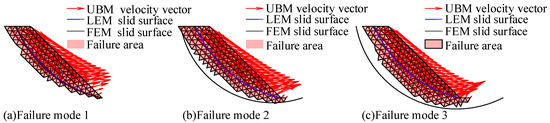
Figure 6.
Homogeneous slope failure modes.
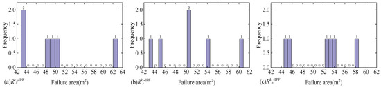
Figure 7.
Histogram of homogeneous slope failure area.
Table 3.
Statistics of homogeneous slope failure modes.
Table 4.
Statistics of homogeneous slope failure risk.
The calculation results show that:
- (1)
- Failure mode 1 is obtained by the UBM, LEM and FEM; however, the other two failure modes are not obtained by the LEM. This is because the LEM calculates slope stability under random samples of shear strength parameter based on the pre-assumed critical sliding surface and therefore its failure mode is not a real failure mode. The FEM obtained similar calculation results as the proposed method; however, the FEM method needed to build a finite element model satisfying the static equilibrium condition, strain compatibility condition and constitutive relation of soil mass when analyzing slope stability. Unfortunately, the constitutive relation of soil mass is complex and there is no unified constitutive model to characterize it at present. In addition, the FEM contains more human factors when judging slope failure modes.
- (2)
- Three slope failure modes are obtained based on , and by the UBM. The failure probability of each failure mode is equal, but there are slight differences in the failure risk of each failure mode and overall failure risk. Theoretically, there is only one slope limit state under the action of each random field, which corresponds to a unique external overload coefficient, bulk overload coefficient and slope stability coefficient. However, due to the influence of calculation errors, rounding errors and calculation accuracy, the accumulation of subtle differences is caused.
- (3)
- Table 4 compares the calculation results of the UBM, LEM and FEM. It can be observed that the failure risk obtained by Equations (14) and (20) based on the UBM are the same. However, it should be noted that Equation (14) is the slope failure risk calculation based on IFP. Therefore, it is necessary to first count all slope failure modes, including the failure risk coefficient and failure probability of each failure mode; Equation (20) is the slope failure risk calculation based on EFP by the failure probability and failure risk coefficient of each discrete element, which can be easily obtained via the element failure function Equations (15)–(17) and the element failure probability Equation (18) proposed in this paper.
3.2. Case 2: A Heterogeneous Slope
3.2.1. Heterogeneous Slope Description
Figure 8 shows a slope with a height of 24 m, a top width of 40 m and a slope ratio of 3:4. Many scholars have calculated and analyzed this slope [34,35,36]; however, there is no systematic analysis and research on the ultimate bearing capacity. For this reason, the ultimate bearing capacity and slope failure risk are studied based on the proposed method. The slope’s undrained shear strength is set as a random quantity and assume to have lognormal distribution. The mean value of the undrained shear strength of the upper and lower layers of the slope is 70 kPa and 100 kPa, respectively, and the standard deviation is 21 kPa and 30 kPa, respectively. Using non-common-node finite elements discrete to the slope, 1508 finite elements, 4524 non-common nodes and 2409 discontinuities are obtained. The soil capacity γ is set to a constant value of 19.0 kN/m3, and other calculation parameters are shown in Table 5. The quantity of random fields nm = 2000, and Equation (7) was used to obtain the 2000 random fields.
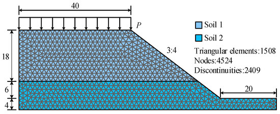
Figure 8.
Heterogeneous slope calculation model.
Table 5.
Statistics of soil parameters.
3.2.2. Result of Heterogeneous Slope
The slope stability resulting from 2000 soil shear strength parameter random fields is calculated by running the UBM parallel calculation program on a small workstation. Table 6 list the results obtained by the FEM, LEM and UBM. Figure 9 and Figure 10 give the relationship between top load, bulk density and the stability slope coefficient respectively when . Figure 11 gives the histogram of the external overload coefficient , bulk overload coefficient and slope stability coefficient .
Table 6.
Comparison of slope reliability results of different methods.
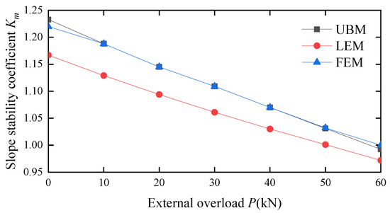
Figure 9.
Relationship between external load and slope stability coefficient of heterogeneous slope.
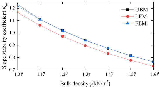
Figure 10.
Relationship between bulk density and slope stability coefficient of heterogeneous slope.
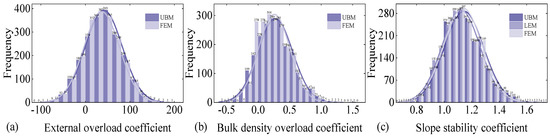
Figure 11.
Histogram of , and of heterogeneous slope.
The calculation results show that:
- (1)
- The slope reliability results of different methods are compared in Table 6. It can be observed that the slope failure probability base on , and obtained via the UBM is essentially consistent with low rates of error. From the upper limit theorem, the slope failure probability calculated by the UBM will slightly underestimate the true solution. The results obtained via the UBM are greater than those obtained via the FEM when calculating the bulk density overload coefficient and slope stability coefficient. The main reason is that the FEM relies on iteration non-convergence, plastic zone penetration and node displacement mutation as judgment criteria when analyzing slope stability. Therefore, the results are not necessarily strictly accurate solutions and their values may be greater than the upper limit solutions obtained by the UBM.
- (2)
- Based on the , and , the slope failure probability can be calculated, which is close or equal. From the perspective of calculation efficiency, the above three methods in this paper can carry out large-scale parallel calculation. However, it required 2.16 h (roughly 86.4 h for single thread calculation), 2.19 h (roughly 87.6 h for single thread calculation) and 17.28 h (roughly 691.2 h for single thread calculation) to calculate the , and of 1000 random field samples. It required 118.0, 122.3 and 472.6 h, respectively, to calculate the , and by the FEM for the same sample.
- (3)
- Figure 10 and Figure 11 reflect the process of gradually increasing the top load and bulk density to cause the slope to reach the limit state. It can be observed intuitively that with the gradual increase of top load P and bulk density γ, the slope stability coefficient obtained via the UBM, LEM and FEM all show a decreasing trend, and the results obtained via the UBM and FEM are close to each other, which are all greater than the results calculated by the LEM.
- (4)
- Figure 11 gives the histogram of , and . It can be intuitively observed that , and all present the characteristics of lognormal distribution, being high in the center and low on both sides.
The LEM’s default is that there is only one slope failure mode, as depicted by the blue line in Figure 12; three slope failure modes can be obtained simultaneously by the FEM, as depicted by the black line in Figure 12. The most significant advantage of the proposed method is that it can capture all the slope failure modes simultaneously. By calculating 1000 groups of slope random field samples, a total of three slope failure modes are obtained, as depicted by the pink area in Figure 12. The histogram of the slope failure area is shown in Figure 13. Table 7 lists the statistics of slope failure modes by IFP method. Table 4 lists the statistics of the slope failure risk.
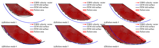
Figure 12.
Heterogeneous Slope failure modes.
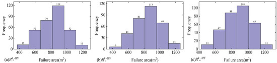
Figure 13.
Histogram of s Heterogeneous lope failure area.
Table 7.
Statistics of heterogeneous slope failure modes.
The calculation results show that:
- (1)
- Only failure mode 4 is obtained by the LEM while the other five failure modes are not obtained. This is because the LEM calculates slope stability under random samples of shear strength parameter based on the pre-assumed critical sliding surface, and therefore its failure mode is not a genuine failure mode. Failure modes 1, 4 and 6 are obtained simultaneously by the FEM while the other three failure modes are not obtained. This is because the FEM needed to build a finite element model satisfying the static equilibrium condition, strain compatibility condition and constitutive relation of soil mass when analyzing slope stability. Therefore, on the basis of the known slope constitutive model, more accurate calculation results can be obtained than with the LEM or UBM. Unfortunately, the constitutive relation of soil mass is complex and there is no unified constitutive model to characterize it at present. In addition, the FEM contains more human factors when judging slope failure modes.
- (2)
- Six slope failure modes are obtained based on , and by the UBM. There are slight differences in the failure probability of each failure mode, the failure risk of each failure mode and overall failure risk. Theoretically, there is only one slope limit state under the action of each random field, which corresponds to the only external overload coefficient, bulk overload coefficient and slope stability coefficient. However, due to the influence of calculation errors, rounding errors and calculation accuracy, the accumulation of subtle differences is caused.
- (3)
- Table 8 compares the calculation results of the UBM, LEM and FEM. It can be seen that the failure risk obtained by Equations (14) and (20) based on UBM are the same. However, it should be noted that Equation (14) is the slope failure risk calculation based on IFP. Therefore, it is necessary to first count all slope failure modes, including the failure risk coefficient and failure probability of each failure mode; Equation (20) is the slope failure risk calculation based on EFP by failure probability and failure risk coefficient of each discrete element, which can be easily obtained by the element failure function Equations (15)–(17) and the element failure probability Equation (18) proposed in this paper.
Table 8. Statistics of heterogeneous slope failure risk.
4. Discussion
An efficient method for calculating slope failure risk based on element failure probability is proposed in this paper, which uses , and to judge the instability of slope, and uses velocity field obtained via the UBM to locate each failure element. The problem of solving the failure probability and failure risk coefficient of each failure mode is transformed into the problem of solving the element failure probability and failure risk coefficient of discrete elements, which greatly simplifies the calculation process. In addition, according to the definition of limit state, the element failure function is established based on , and [18]. It can be observed from the calculation process of , and (as shown in Figure 1) that and are only solved once for large-scale linear programming problems, while usually requires solving and many times and therefore the failure risk computational efficiency based on and are greatly improved.
The analysis of the two cases shows that the results obtained via the UBM based on , and are very close, with a low rate of error (<5%). Theoretically, the slope failure risk coefficient under each sample should be consistent; that is, the obtained results should be equal. However, load distribution type, action form and calculation accuracy may affect the results. When using Geo-studio software for failure risk comparative analysis, the critical sliding surface obtained from the mean value of soil shear strength parameters is used to analyze all samples [5]. In addition, the LEM only considers one-dimensional spatial variability of the sliding surface and therefore its calculation results are worthy of discussion [20]. The most accurate result can be obtained by 8-node FEM based on OptumG2 on the basis of the known soil constitutive relationship. However, unfortunately, the soil constitutive relationship is complicated and the failure mode screening involves many human factors [4,17]. It should be noted that the UBM computation program in this paper can implement parallel computation in Python and therefore the computation efficiency can be greatly improved.
The proposed method is mainly aimed at soil slope, but the failure of rock slope is mainly affected by the cohesion, friction angle and bulk density of the structural plane [4,35]. The study of efficient rock slope failure risk analysis will be the focus of subsequent work. In addition, earthquake and groundwater are the main causes of slope instability [5,21,27] and therefore it is also urgent to study efficient failure risk analysis methods under the action of earthquake and groundwater.
5. Conclusions
A slope failure risk analysis method based on EFP was proposed. A UBM parallel calculation program is prepared in Python to obtain the distribution law of external overload coefficient, bulk overload coefficient and slope stability coefficient, which provided an efficient calculation method for slope failure risk. Through in-depth analysis of two examples of homogeneous slope and heterogeneous slope, the effectiveness of the proposed method is verified, and its main conclusions are as follows:
- (1)
- The slope failure risk calculation method based on EFP provides engineers with practical reference significance for reinforcement design and risk assessment by counting the possibility of slope failure through , and and the difference in the spatial distribution of the slope failure area through the information of element location.
- (2)
- Compared with traditional failure risk analysis methods, the proposed method based on EFP can not only effectively avoid the problem of the stability coefficient between multi-failure modes and the correlation between slide volume, but also accurately quantify the failure risk of slope multi-failure modes. In particular, when calculating the overall failure risk of slope with multi-failure modes, it can be obtained only according to the failure probability and the failure risk coefficient (the area of the area) of the element, avoiding the statistics of failure modes and the calculation of the failure risk coefficient (the area of each failure mode). This method has important theoretical value for slope failure risk assessment.
- (3)
- The traditional LEM has a high rate of error in the failure risk analysis of a heterogeneous slope. In this study, the failure of the slope element is judged by the double attributes of , , and the centroid velocity of the element. The failure of the slope is judged by , and and the failure area of the slope is located via the centroid velocity of the element. This method can capture all potential slope failure modes simultaneously, thus obtaining more reasonable results than the LEM.
- (4)
- The failure risk of a slope is essential in order to calculate the influence caused by the slope failure. In this paper, only the area is used to measure the slope failure risk and other factors are ignored, such as the importance of the slope, the environmental impact assessment, the vulnerability of the bearing body, etc. Although a simplified failure consequence assessment method is adopted, it does not affect the applicability of the proposed method. If there is a more accurate element failure consequence, it should simply be replaced.
- (5)
- It should be noted that the UBM parallel computing program prepared in Python can make full use of the advantages of multi-threaded parallel computing on a small workstation. Theoretically, it could call 64 threads at the highest level for parallel computing of each sample, but only 42 threads are called due to other operational requirements. When GEO-studio software is called by MATLAB to calculate each sample, random fields need first to be generated through pre-processing, then the calculation of each sample is carried out on this basis. The 8-node FEM based on OptumG2 can only obtain the result of one sample each time and cannot carry out large-scale parallel calculation.
Author Contributions
Conceptualization, P.P., Z.L., X.Z., W.Z. and W.D.; methodology, X.Z.; software, P.P. and Z.L.; validation, X.Z.; formal analysis, P.P.; investigation, P.P. and Z.L.; resources, Z.L. and X.Z.; data curation, W.D.; writing—original draft preparation, P.P. and Z.L.; writing—review and editing, P.P. and Z.L.; visualization, X.Z. and W.Z.; supervision, P.P., W.Z. and Z.L.; project administration, X.Z. and W.D.; funding acquisition, Z.L. and X.Z. All authors have read and agreed to the published version of the manuscript.
Funding
This research was funded by the National Natural Science Foundation of China, grant number 12162018 and 12262016.
Institutional Review Board Statement
Not applicable for studies not involving humans or animals.
Informed Consent Statement
Not applicable.
Data Availability Statement
Not applicable.
Conflicts of Interest
The authors declare no conflict of interest.
Nomenclature
The following symbols are used in this paper:
| = | cohesion before strength reduction | |
| = | cohesion after strength reduction | |
| = | the cohesion of the triangular element e in the th non-Gaussian random field | |
| = | the cohesion of the triangular element e in the th standard Gaussian random field | |
| C | = | the failure risk coefficient |
| = | failure risk coefficient of slope element e | |
| = | failure risk coefficient of the k-th failure mode | |
| = | the coordinate transformation matrix of the finite element b on the boundary | |
| = | the matrix of plastic flow constraint conditions of the velocity discontinuity d | |
| = | the matrix of plastic flow constraint conditions of the velocity discontinuity d | |
| = | the matrix of plastic flow constraint conditions of the finite element e | |
| = | the matrix of plastic flow constraint conditions of the finite element e | |
| = | the actual load of the slope | |
| = | the external load when the slope is in the limit state | |
| = | correlated non-Gaussian random fields | |
| = | correlated standard Gaussian random fields | |
| = | the slope failure function based on IFP of km | |
| = | the slope failure function based on IFP of kF | |
| = | the slope failure function based on IFP of kγ | |
| = | failure function based on km -uc-EFP of the element e in the th random field | |
| = | failure function based on kF-uc-EFP of the element e in the th random field | |
| = | failure function based on kγ-uc-EFP of the element e in the th random field | |
| = | the external force overload coefficient of the slope | |
| = | the stability coefficient of the slope | |
| = | the bulk density overload coefficient of the slope | |
| = | the external force overload coefficient of th random field | |
| = | the stability coefficient of th random field | |
| = | the bulk density overload coefficient of th random field | |
| = | the fluctuation ranges in the horizontal coordinate direction | |
| = | the fluctuation ranges in the vertical coordinate direction | |
| = | the shear strength parameter of soil mass | |
| = | ||
| = | the quantity of cohesion and internal friction angle random fields of soil material | |
| = | the quantity of finite elements on the boundary of slope | |
| = | the quantity of velocity discontinuities | |
| = | the quantity of finite elements | |
| = | the quantity of failure modes | |
| = | pore water pressures at the i-th node of the finite element e (i = 1,2,3) | |
| = | failure probability of slope | |
| = | failure probability of slope element e | |
| = | failure probability of the k-th failure mode | |
| = | slope failure risk by M-IFP | |
| = | slope failure risk by M-uc-EFP | |
| = | failure risk of slope element e | |
| = | failure risk of the k-th failure mode | |
| = | the mean value of cohesion with lognormal distribution | |
| = | velocity of the element in the th random field | |
| = | the mean value of internal friction angle with lognormal distribution | |
| = | the mean value of lognormal distribution of | |
| = | the mean value of normal variables of | |
| = | the mean value of normal variables of | |
| = | the mean value of the corresponding normal variable of | |
| = | the mean value of M | |
| = | the velocity vector of the boundary finite element b | |
| = | the velocity vector of the velocity discontinuity d | |
| = | the velocity vector of finite element e | |
| = | the internal power of finite elements | |
| = | the internal power of the velocity discontinuities | |
| = | the external work power done by the external load or dead weight on the velocity of the finite element nodes | |
| = | the horizontal coordinates of element a | |
| = | the horizontal coordinates of element b | |
| = | the vertical coordinates of element a | |
| = | the vertical coordinates of element b | |
| = | the limit state function obtained by gradually increasing the external load of the slope | |
| = | the limit state function obtained by gradually reducing the shear strength parameters of soil materials | |
| = | the limit state function obtained by gradually increasing the slope load | |
| = | the plastic multiplier | |
| = | the decision variable | |
| = | the actual bulk density of the slope | |
| = | the bulk density when the slope is in the limit state | |
| internal friction angle before strength reduction | ||
| = | internal friction angle after strength reduction | |
| = | the internal friction angle of the triangular element e in the th non-Gaussian random field | |
| = | the internal friction angle of the triangular element e in the th standard Gaussian random field | |
| = | the standard deviation of cohesion with lognormal distribution | |
| = | the standard deviation of internal friction angle with lognormal distribution | |
| = | the standard deviation of lognormal distribution of | |
| = | the mean value of normal variables of | |
| = | the standard deviation value of normal variables of | |
| = | the standard deviation of the corresponding normal variable of | |
| = | the standard deviation of M |
References
- Intrieri, E.; Carlà, T.; Gigli, G. Forecasting the time of failure of landslides at slope-scale: A literature review. Earth-Sci. Rev. 2019, 193, 333–349. [Google Scholar] [CrossRef]
- Maxwell, A.E.; Sharma, M.; Kite, J.S.; Donaldson, K.A.; Thompson, J.A.; Bell, M.L.; Maynard, S.M. Slope Failure Prediction Using Random Forest Machine Learning and LiDAR in an Eroded Folded Mountain Belt. Remote Sens. 2020, 12, 486. [Google Scholar] [CrossRef]
- Kolapo, P.; Oniyide, G.O.; Said, K.O.; Lawal, A.I.; Onifade, M.; Munemo, P. An Overview of Slope Failure in Mining Operations. Mining 2022, 2, 350–384. [Google Scholar] [CrossRef]
- Li, Z.; Hu, Z.; Zhang, X.; Du, S.; Guo, Y.; Wang, J. Reliability analysis of a rock slope based on plastic limit analysis theory with multiple failure modes. Comput. Geotech. 2019, 110, 132–147. [Google Scholar] [CrossRef]
- Peng, P.; Li, Z.; Zhang, X.Y.; Shen, L.F.; Xu, Y. Research on element failure probability and failure mode of soil slope. Eng. Mech. 2022, 39, 1–15. [Google Scholar] [CrossRef]
- Li, D.-Q.; Yang, Z.-Y.; Cao, Z.-J.; Zhang, L.-M. Area failure probability method for slope system failure risk assessment. Comput. Geotech. 2018, 107, 36–44. [Google Scholar] [CrossRef]
- Ji, J.; Zhang, W.; Zhang, F.; Gao, Y.; Lü, Q. Reliability analysis on permanent displacement of earth slopes using the simplified Bishop method. Comput. Geotech. 2019, 117, 103286. [Google Scholar] [CrossRef]
- Liu, X.; Li, D.-Q.; Cao, Z.-J.; Wang, Y. Adaptive Monte Carlo simulation method for system reliability analysis of slope stability based on limit equilibrium methods. Eng. Geol. 2019, 264, 105384. [Google Scholar] [CrossRef]
- Ching, J.; Phoon, K.-K.; Hu, Y.-G. Efficient Evaluation of Reliability for Slopes with Circular Slip Surfaces Using Importance Sampling. J. Geotech. Geoenviron. Eng. 2009, 135, 768–777. [Google Scholar] [CrossRef]
- Dyson, A.P.; Tolooiyan, A. Comparative Approaches to Probabilistic Finite Element Methods for Slope Stability Analysis. Simul. Model. Pr. Theory 2019, 100, 102061. [Google Scholar] [CrossRef]
- Wang, M.-Y.; Li, D.-Q.; Tang, X.-S.; Liu, Y. Modeling Irregularly Inclined Fissure Surfaces within Nonuniform Expansive Soil Slopes. Int. J. Géoméch. 2022, 22, 04022124. [Google Scholar] [CrossRef]
- Griffiths, D.V.; Huang, J.; Fenton, G.A. Influence of Spatial Variability on Slope Reliability Using 2-D Random Fields. J. Geotech. Geoenviron. Eng. 2009, 135, 1367–1378. [Google Scholar] [CrossRef]
- Lysmer, J. Limit Analysis of Plane Problems in Soil Mechanics. J. Soil Mech. Found. Div. 1970, 96, 1311–1334. [Google Scholar] [CrossRef]
- Chen, W.F. Limit Analysis and Soil Plasticity; Elsevier Science: Amsterdam, The Netherlands, 1975. [Google Scholar]
- Sloan, S.W. Lower bound limit analysis using finite elements and linear programming. Int. J. Numer. Anal. Methods Géoméch. 1988, 12, 61–77. [Google Scholar] [CrossRef]
- Sloan, S.; Kleeman, P. Upper bound limit analysis using discontinuous velocity fields. Comput. Methods Appl. Mech. Eng. 1995, 127, 293–314. [Google Scholar] [CrossRef]
- Li, Z.; Zhou, Y.; Guo, Y. Upper-Bound Analysis for Stone Retaining Wall Slope Based on Mixed Numerical Discretization. Int. J. Géoméch. 2018, 18. [Google Scholar] [CrossRef]
- Zhang, X.Y.; Zhang, L.X.; Li, Z. Reliability analysis of soil slope based on upper bound method of limit analysis. Rock Soil Mech. 2018, 39, 1840–1850. [Google Scholar] [CrossRef]
- Li, L.; Liu, B.C. Lower bound limit analysis on bearing capacity of slope and its reliability. Chin. J. Rock Mech. Eng. 2001, 20, 508–513. [Google Scholar]
- Chen, Z.H.; Lei, J.; Huang, J.H.; Cheng, X.H.; Zhang, Z.C. Finite element limit analysis of slope stability considering spatial variability of soil strengths. Chin. J. Geotech. Eng. 2018, 40, 985–993. [Google Scholar] [CrossRef]
- Li, Z.; Chen, Y.; Guo, Y.; Zhang, X.; Du, S. Element Failure Probability of Soil Slope under Consideration of Random Groundwater Level. Int. J. Géoméch. 2021, 21, 04021108. [Google Scholar] [CrossRef]
- Chu, X.; Li, L.; Cheng, Y.-M. Risk Assessment of Slope Failure Using Assumption of Maximum Area of Sliding Mass and Factor of Safety Equal to Unit. Adv. Civ. Eng. 2019, 2019, 1–11. [Google Scholar] [CrossRef]
- Apostu, I.-M.; Lazar, M.; Faur, F. A Suggested Methodology for Assessing the Failure Risk of the Final Slopes of Former Open-Pits in Case of Flooding. Sustainability 2021, 13, 6919. [Google Scholar] [CrossRef]
- Silva, F.; Lambe, T.W.; Marr, W.A. Probability and Risk of Slope Failure. J. Geotech. Geoenviron. Eng. 2008, 134, 1691–1699. [Google Scholar] [CrossRef]
- Cassidy, M.J.; Uzielli, M.; Lacasse, S. Probability risk assessment of landslides: A case study at Finneidfjord. Can. Geotech. J. 2008, 45, 1250–1267. [Google Scholar] [CrossRef]
- Zhou, J.; Qin, C. Finite-element upper-bound analysis of seismic slope stability considering pseudo-dynamic approach. Comput. Geotech. 2020, 122, 103530. [Google Scholar] [CrossRef]
- Zhou, J.; Qin, C. Stability analysis of unsaturated soil slopes under reservoir drawdown and rainfall conditions: Steady and transient state analysis. Comput. Geotech. 2021, 142, 104541. [Google Scholar] [CrossRef]
- Jiang, S.H.; Li, D.Q.; Zhou, C.B.; Fang, G.G. Slope reliability analysis considering effect of autocorrelation functions. Chin. J. Geotech. Eng. 2014, 36, 508–518. [Google Scholar] [CrossRef]
- Wang, X.; Xia, X.; Zhang, X.; Gu, X.; Zhang, Q. Probabilistic Risk Assessment of Soil Slope Stability Subjected to Water Drawdown by Finite Element Limit Analysis. Appl. Sci. 2022, 12, 10282. [Google Scholar] [CrossRef]
- Li, D.-Q.; Jiang, S.-H.; Cao, Z.-J.; Zhou, W.; Zhou, C.-B.; Zhang, L.-M. A multiple response-surface method for slope reliability analysis considering spatial variability of soil properties. Eng. Geol. 2015, 187, 60–72. [Google Scholar] [CrossRef]
- Griffiths, D.V.; Fenton, G.A. Influence of Soil Strength Spatial Variability on the Stability of an Undrained Clay Slope by Finite Elements. In Slope Stability 2000; American Society of Civil Engineers: Reston, VI, USA, 2000. [Google Scholar] [CrossRef]
- Pan, Y.; Liu, Y.; Tyagi, A.; Lee, F.-H.; Li, D.-Q. Model-independent strength-reduction factor for effect of spatial variability on tunnel with improved soil surrounds. Géotechnique 2021, 71, 406–422. [Google Scholar] [CrossRef]
- Jiang, S.H.; Pan, J.M.; Qin, G.Q. Reliability analysis of spatially variable soil slopes based on representative slip surfaces. Eng. J. Wuhan Univ. 2016, 49, 768–773. [Google Scholar]
- Huang, J.; Lyamin, A.; Griffiths, D.V.; Krabbenhoft, K.; Sloan, S. Quantitative risk assessment of landslide by limit analysis and random fields. Comput. Geotech. 2013, 53, 60–67. [Google Scholar] [CrossRef]
- Cheng, H.; Chen, J.; Chen, R.; Chen, G.; Zhong, Y. Risk assessment of slope failure considering the variability in soil properties. Comput. Geotech. 2018, 103, 61–72. [Google Scholar] [CrossRef]
- Ali, A.; Lyamin, A.V.; Huang, J.; Li, J.H.; Cassidy, M.J.; Sloan, S.W. Probabilistic stability assessment using adaptive limit analysis and random fields. Acta Geotech. 2016, 12, 937–948. [Google Scholar] [CrossRef]


Disclaimer/Publisher’s Note: The statements, opinions and data contained in all publications are solely those of the individual author(s) and contributor(s) and not of MDPI and/or the editor(s). MDPI and/or the editor(s) disclaim responsibility for any injury to people or property resulting from any ideas, methods, instructions or products referred to in the content. |
© 2023 by the authors. Licensee MDPI, Basel, Switzerland. This article is an open access article distributed under the terms and conditions of the Creative Commons Attribution (CC BY) license (https://creativecommons.org/licenses/by/4.0/).