Slope Deflection Method in Nonlocal Axially Functionally Graded Tapered Beams

Abstract

In this study, the slope deflection method was presented for structures made of small-scaled axially functionally graded beams with a variable cross section within the scope of nonlocal elasticity theory. The small-scale effect between individual atoms cannot be neglected when the structures are small in size. Therefore, the theory of nonlocal elasticity is used throughout. The stiffness coefficients and fixed-end moments are calculated using the method of initial values. With this method, the solution of the differential equation system is reduced to the solution of the linear equation system. The given transfer matrix is unique and the problem can be easily solved for any end condition and loading. In this problem, double integrals occur in terms of the transfer matrix. However, this form is not suitable for numerical calculations. With the help of Cauchy’s repeated integration formula, the transfer matrix is given in terms of single integrals. The analytical or numerical calculation of single integrals is easier than the numerical or analytical calculation of double integrals. It is demonstrated that the nonlocal effect plays an important role in the fixed-end moments of small-scaled beams.

1. Introduction

In the present study, static analysis of axially graded nonlocal Euler–Bernoulli beams was performed using the slope deflection method. Firstly, the basic equations of a nonlocal Euler–Bernoulli beam subjected to distributed load are obtained [1,2,3,4]. Then, it is assumed that the modulus of elasticity and the moment of inertia functionally change along the axis (AFGM) in order to provide a general solution to the problem. For the solution to the problem, the transport matrix is formed with the help of Cauchy’s repeated integral. Stiffness coefficients were obtained by examining different boundary conditions for different loads. Although there are many studies on axially graded beams in previous studies, there is no research in the literature on the solution of unit displacement constants of nanoscale frames. In the above-mentioned studies, the slope deflection method has been solved for beams with constant cross sections and includes a classical structural solution. In the present work, the equations are given in the most general form and the solutions can be easily solved independently of the changes in the cross section and material parameters. Moreover, as this study is examined within the scope of nonlocal elasticity theory for Euler–Bernoulli beams, it brings great innovation to the literature in terms of static analysis of both macro- and nano-scale systems.

There are many approaches to solving mechanical problems. Most of these theories are methods used in classical elasticity theory. However, this situation differs in the analysis of nanoscale structures. It has been repeatedly emphasized that the effect of atomic size should be taken into account in the analysis of nanoscale structures. In this context, approaches suggesting enriched deformation theories such as nonlocal elasticity theory, Reddy’s higher-order deformation theory, and strain gradient theory have been put forward by early researchers in analyzing such structures [5].

In the literature, there are many methods for solving statically indeterminate systems, such as the force method and the slope deflection method. The slope deflection method is the most widely used among these approaches, especially for systems with a high degree of hyperstaticity.

Simplifying the application of the slope deflection method, new reduced equations based on incorporating both the rotations of the joints and the effects of fixed-end moments into one term instead of two terms are presented [6]. The slope deflection method was first introduced by George A. Maney to analyze beam and frame systems in the early 20th century. This method is basically based on the solution of the continuity equations obtained depending on the displacements of the joints in beam and frame systems. The main advantage of this method is that it can be easily applied to statically indeterminate systems and is suitable for programming [7,8,9]. Statically indeterminate space frame systems were analyzed using the slope deflection method [10]. The slope deflection method was used by the researchers to analyze the orthotropic bridge support plates analytically [11]. Static analyses of Timoshenko beam–column connections were investigated using the slope deflection method [12].

With the developing technology, smart materials have replaced the traditional materials used in engineering problems. It is of great importance to determine the properties of advanced technology materials such as functionally graded materials at a good level in order for the structural elements used in almost every field of engineering to have higher mechanical strength.

AFGMs are advanced technology materials used in building elements such as wind turbines, helicopter blades, and airframes. Studies have shown that AFGMs subjected to loads in different directions show a higher mechanical strength than metal-ceramic-type FGMs. However, owing to the fact that the equations of motion of AFGMs can take very complex forms, their analytical analysis is quite difficult [13,14,15,16]. In the studies conducted by the researchers, notably in the last few decades, it has been observed that the resistance of axially graded beams to buckling and dynamic behavior is better than that of isotropic beams. Researchers analyzed the vibration behavior of AFGM beams using a variation iteration approach [17]. The buckling behavior of a composite beam subjected to an axially varying load type was investigated using the Ritz method [18]. A group of researchers investigated the buckling and vibration behavior of axially graded GPL composite beams using the Ritz method. In this context, the mechanical behavior of Timoshenko beams for five different load types was examined and, at the end of the study, it was revealed that the grading pattern depends not only on the buckling load, but also on the grading type of the load (AVLs) [19]. The natural frequencies of a rotating AFGM beam are investigated within the scope of nonlocal elasticity theory [20]. At the end of the study, it was seen that the grading parameter has a significant effect on the free vibration behavior of the beams.

Static analysis of an AFGM beam is numerically solved [21]. The mechanical behavior of axially graded metal–ceramic microbeams is studied with the help of a higher-order theory [22]. The vibration character of an AFGM beam reinforced by CNTs was investigated using a differential approximation method. The study revealed that the frequency value is very sensitive to the volume fraction of CNTs [23]. The vibration behavior of AFGM beams reinforced with GPLs has been investigated within the context of Reddy’s higher-order deformation theory [24]. The natural frequency values of AFGM beams reinforced with GPLs have been investigated in previous studies [25]. Many structural elements are exposed to mechanical effects such as bending, buckling, torsion, vibration, and thermal change due to external conditions. In order to minimize such effects, the geometry and specific properties of the building elements used should be thoroughly analyzed.

The buckling behavior of sandwich beams subjected to axially variable load has been demonstrated by a series of studies [26]. The dynamic response of a laminated composite beam under axially varying loads (AVLs) is studied with the help of a higher-order deformation theory [27]. The effect of porosity shape on the buckling and free vibration behavior of a functionally graded beam was investigated [28]. The buckling and dynamic characteristics of porous beams reinforced with GPLs were investigated, and it was reported that porosity shape and axially varying loads have a sensitive effect on these behaviors [29]. A new approach is proposed for the free vibration behavior of a non-uniform AFGM beam [30]. The modal behavior of a three-dimensional FGM beam is obtained using the finite element method [31]. The natural frequencies of the exponential FGM beams are presented with an analytical solution method [32]. The free vibration behavior of AFGM beams under different boundary conditions has been demonstrated in studies [33].

Functionally graded materials were first introduced by a group of researchers in the Sendai region of Japan and have attracted the interest of researchers [34]. With their unique physical and mechanical properties, FGMs have significant potential in the field of mechanics in the analysis of building materials. Previous studies have demonstrated the mechanical behavior of FGM structures such as bending, buckling, vibration, and thermal stress. Investigations have clearly demonstrated the analysis of FGM structures under different loading conditions within many studies. In the study presented here, the subject was investigated with a different approach related to the work of the researchers and briefly discussed [35]. A study conducted by early researchers demonstrated the elasticity solution of Euler–Bernoulli beams made of FGM subjected to a transverse load [36]. The thermal buckling and vibration behavior of a sandwich plate with a viscoelastic core have been studied by taking into account the effect of temperature [37]. Researchers studied the thermoelastic behavior of FGM beams by obtaining polynomials of the exact results of different equations expressed with interpolation functions [38]. Wave propagation behavior of FGM beams under high-frequency loading was analyzed using a finite element approach [39]. The ambient-temperature-dependent static behavior of beams in an FGM structure was investigated with the help of a high-order beam theory [40]. A new model was presented for calculating the buckling load of columns made of FGMs [41]. The mechanical behavior of Euler–Bernoulli beams was presented in which material properties vary in either the horizontal or vertical direction [42]. Functionally graded materials are a type of composite material whose material properties are designed to show continuity from one surface to another. As for laminated structures, stress discontinuities occur between two surfaces. These discontinuities are eliminated in FGMs. Owing to these properties, FGMs are widely used today in many areas such as the design of medical devices, as well as in the fields of construction and ship and aircraft engineering. Beams made of FGMs are classified into two basic groups according to their design status and their grading according to the thickness and length of the element, with their mechanical properties varying in different directions (axially or longitudinal) [43,44]. These types of beams are called axially graded beams (AFGs). There are a limited number of studies in the literature on the analytical approach of AFGs [45,46]. There are many methods in the literature to determine the natural frequency of non-uniform axial FGM beams. The bending and buckling behaviors of bi-directional FGM beams are investigated within the scope of strain gradient theory [47,48]. These are the complementary functions approach [49], finite element method [42,43,44,45,46,47,48,49,50], power series approach [51] used to define mode shapes, Chebyshev polynomials [52], differential quadrature method [53], differential form including initial values [54], and Fredholm integral equations [55]. Classical elasticity theory is not sufficient to analyze the behavior of nanoscale structures in the most accurate way. Therefore, it has emerged that an enriched continuum model is needed to describe the mechanical behavior of such structures. Although the molecular dynamics approach (MD) is a method used to analyze such structures, it contains a high level of computational load, making it difficult for such simulations to express a general solution. The nonlocal elasticity theory approach states that the stress field at a point is affected not only by the strain at that point, but also by the strain of all adjacent points. In this context, nonlocal elasticity theory has an important place in the analysis of size-dependent mechanical behavior [56,57]. In recent years, numerous studies are presented to display the importance of the size effect in small-scale structures [58,59,60]. The slope deflection method is a method based on expressing the displacement components at the nodes as unknowns. There are many publications in the literature related to this method. However, there is no publication describing the method in nonlocal theory for structures composed of AFG elements. Stiffness coefficients and end moments are analyzed within the scope of nonlocal elasticity theory using the method of initial values (MIV).

2. Basic Equations

The basic Equation (1) [1,2,5] of a nonlocal Euler–Bernoulli beam is as

$$\frac{dv}{dz}=\phi , \frac{d\phi }{dz}=-\frac{M-{\gamma }^2{M}^{″}}{E(z)I(z)}, \frac{dM}{dz}=T, \frac{dT}{dz}=-p(z)$$

(1)

Note that $v$, $\phi$, $M$, $T$, $E(z)$, $I(z)$, and $\gamma$ are deflection, rotation, moment, shear force, modulus of elasticity, moment of inertia, and small-scale parameter revealing a small-scale effect on the response of structures in nano size, respectively. Here, $p(z)$ is the distributed load [61,62,63,64,65,66,67,68]. Using Equation (1), the above expression can be written as

$$\frac{d}{dz}\left(\begin{array}{c}v\\ \phi \\ M\\ T\end{array}\right)=\left[\begin{array}{cccc}0& 1& 0& 0\\ 0& 0& -\frac{1}{E(z)I(z)}& 0\\ 0& 0& 0& 1\\ 0& 0& 0& 0\end{array}\right]\left(\begin{array}{c}v\\ \phi \\ M\\ T\end{array}\right)+\left[\begin{array}{c}0\\ -\frac{{\gamma }^{2}p(z)}{E(z)I(z)}\\ 0\\ -p(z)\end{array}\right]$$

(2)

Equation (2) can be expressed as

$$\frac{d\overrightarrow{y}}{dz}=\underset{˜}{A}\overrightarrow{y}+\overrightarrow{f}, y(0)={\overrightarrow{y}}_0$$

(3)

The solution of the MIV given by Equation (3) is

$$\overrightarrow{y}(z)=T\underset{˜}{M}(z).{\overrightarrow{y}}_0+{\displaystyle {\int }_0^{z}T\underset{˜}{M}(z-\tau )}.\overrightarrow{f}(\tau )d\tau$$

(4)

where $\tau$ is parameter used on variables in double integrals, $\alpha$ is a variable that shows the variation of E and I along the axis, and $T\underset{˜}{M}(z)$ is the transfer matrix. The transfer matrix is obtained for variable $E$ and $I$ using Cauchy’s repeated integration formula as below [63].

$$T\underset{˜}{M}(z)=\left[\begin{array}{cccc}1& z& -{\displaystyle {\int }_0^z\frac{z-\alpha }{E(\alpha )I(\alpha )}d\alpha }& -{\displaystyle {\int }_0^z\frac{\alpha (z-\alpha )}{E(\alpha )I(\alpha )}d\alpha }\\ 0& 1& -{\displaystyle {\int }_0^z\frac{1}{E(\alpha )I(\alpha )}d\alpha }& -{\displaystyle {\int }_0^z\frac{\alpha }{E(\alpha )I(\alpha )}d\alpha }\\ 0& 0& 1& z\\ 0& 0& 0& 1\end{array}\right]$$

(5)

3. Applications of the Initial Values Method

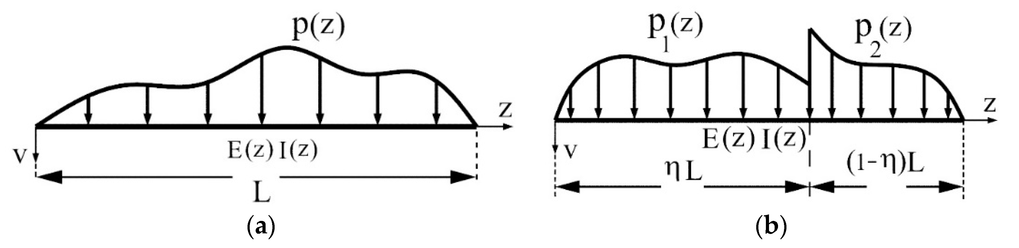
3.1. A Beam Subjected to a Distributed Load

$M_0, T_0, v_0$, and ${\phi }_0$ represent the initial values of the bending moment, shear force, deflection, and rotation, respectively. The unknowns of a beam subjected to a distributed load are calculated using Equations (4) and (5) as below (See Figure 1a).

$$\begin{array}{l}v(z)=-M_0\left({\displaystyle {\int }_0^z\frac{z-\alpha }{E(\alpha )I(\alpha )}d\alpha }\right)+{\displaystyle {\int }_0^{z}p(\tau )}\left({\displaystyle {\int }_0^{z-\tau }-\frac{\alpha (\alpha +\tau -z)}{E(\alpha )I(\alpha )}}d\alpha +\frac{{\gamma }^2(\tau -z)}{E(\tau )I(\tau )}\right)d\tau \\ -T_0\left({\displaystyle {\int }_0^z\frac{\alpha (z-\alpha )}{E(\alpha )I(\alpha )}d\alpha }\right)+v_0+{\phi }_{0}z\end{array}$$

(6)

$$\begin{array}{l}\phi (z)=-M_0\left({\displaystyle {\int }_0^z\frac{1}{E(\alpha )I(\alpha )}d\alpha }\right)-T_0\left({\displaystyle {\int }_0^z\frac{\alpha }{E(\alpha )I(\alpha )}}d\alpha \right)+{\phi }_0\\ +{\displaystyle {\int }_0^{z}p(\tau )}\left({\displaystyle {\int }_0^{z-\tau }\frac{\alpha }{E(\alpha )I(\alpha )}d\alpha -\frac{{\gamma }^2}{E(\tau )I(\tau )}}\right)d(\tau )\end{array}$$

(7)

$$M(z)=M_0+{\displaystyle {\int }_0^{z}p(\tau )(}\tau -z) d(\tau )+T_{0}z, T(z)={\displaystyle {\int }_0^z-p(}\tau ) d(\tau )+T_0$$

(8)

3.2. Beam Subjected to Two Different Distributed Loads

In this case, Equation (4) can be written for both regions as follows (see Figure 1b).

$${\overrightarrow{y}}_1(z)=T\underset{˜}{M}(z).{\overrightarrow{y}}_0+{\displaystyle {\int }_0^{z}T\underset{˜}{M}(z-\tau )}.{\overrightarrow{f}}_1(\tau )d\tau , 0\le z\le \eta L$$

(9)

$${\overrightarrow{y}}_2(z)=T\underset{˜}{M}(z).{\overrightarrow{y}}_1(\eta L)+{\displaystyle {\int }_0^{z}T\underset{˜}{M}(z-\tau )}.{\overrightarrow{f}}_2(\tau )d\tau , 0\le z\le (1-\eta )L$$

(10)

where

$${\overrightarrow{f}}_1(z)=\left(\begin{array}{c}0\\ -\frac{{\gamma }^2{p}_1(z)}{E(z)I(z)}\\ 0\\ -p_1(z)\end{array}\right) , {\overrightarrow{f}}_2(z)=\left(\begin{array}{c}0\\ -\frac{{\gamma }^2{p}_2(z)}{E(z)I(z)}\\ 0\\ -p_2(z)\end{array}\right)$$

(11)

The unknowns of a beam subjected to two distributed loads are calculated using Equations (9) and (10) as below (see Figure 1b).

$$\begin{array}{l}{v}_1(z)=-M_0\left({\displaystyle {\int }_0^z\frac{z-\alpha }{E(\alpha )I(\alpha )}d\alpha }\right)-T_0\left({\displaystyle {\int }_0^z\frac{\alpha (z-\alpha )}{E(\alpha )I(\alpha )}}d\alpha \right)+v_0+{\phi }_{0}z\\ +{\displaystyle {\int }_0^z\frac{p_1(\tau )\left(E(\tau )I(\tau ){\displaystyle {\int }_0^{z-\tau }-\frac{\alpha (\alpha +\tau -z)}{E(\alpha )I(\alpha )}d\alpha +{\gamma }^2(\tau -z)}\right)}{E(\tau )I(\tau )}}d\tau \end{array}$$

(12)

$$\begin{array}{l}{\phi }_1(z)=-M_0\left({\displaystyle {\int }_0^z\frac{1}{E(\alpha )I(\alpha )}d\alpha }\right)-T_0\left({\displaystyle {\int }_0^z\frac{\alpha }{E(\alpha )I(\alpha )}}d\alpha \right)+{\phi }_0\\ +{\displaystyle {\int }_0^z{p}_1}(\tau )\left({\displaystyle {\int }_0^{z-\tau }\frac{\alpha }{E(\alpha )I(\alpha )}d\alpha }-\frac{{\gamma }^2}{E(\tau )I(\tau )}\right)d\tau \end{array}$$

(13)

$$M_1(z)=M_0+{\displaystyle {\int }_0^z{p}_1}(\tau ) (\tau -z) d\tau +T_{o}z, T_1(z)={\displaystyle {\int }_0^z-p_1}(\tau ) d\tau +T_0$$

(14)

$$\begin{array}{l}{v}_2(z)=-M_0\left({\displaystyle {\int }_0^{\eta L}\frac{\eta L-\alpha }{E(\alpha )I(\alpha )}d\alpha }\right)-\left({\displaystyle {\int }_0^z\frac{(z-\alpha )}{E(\alpha )I(\alpha )}}d\alpha \right)\hspace{0.17em}\left({\displaystyle {\int }_0^{\eta L}{p}_1(\tau )(\tau -\eta L)d\tau +\eta L{T}_0+M_0}\right)\\ -M_{0}z\left({\displaystyle {\int }_0^{\eta L}\frac{1}{E(\alpha )I(\alpha )}d\alpha }\right)+{\displaystyle {\int }_0^{\eta L}\frac{p_1(\tau )\left(E(\tau )I(\tau ){\displaystyle {\int }_0^{\eta L-\tau }-\frac{\alpha (\alpha -\eta L+\tau )}{E(\alpha )I(\alpha )}d\alpha +{\gamma }^2(\tau -\eta L)}\right)}{E(\tau )I(\tau )}}d\tau \\ -\left({\displaystyle {\int }_0^z\frac{\alpha (z-\alpha )}{E(\alpha )I(\alpha )}}d\alpha \right)\left({\displaystyle {\int }_0^{\eta L}-p_1(\tau )d\tau +T_0}\right)+z{\displaystyle {\int }_0^{\eta L}{p}_1(\tau )}\left({\displaystyle {\int }_0^{\eta L-\tau }\frac{\alpha }{E(\alpha )I(\alpha )}d\alpha -\frac{{\gamma }^2}{E(\tau )I(\tau )}}\right)d\tau \\ -T_0\left({\displaystyle {\int }_0^{\eta L}\frac{\alpha (\eta L-\alpha )}{E(\alpha )I(\alpha )}d\alpha }+z{\displaystyle {\int }_0^{\eta L}\frac{\alpha }{E(\alpha )I(\alpha )}d\alpha }\right)+{\displaystyle {\int }_0^z\frac{p_2(\tau )\left(E(\tau )I(\tau ){\displaystyle {\int }_0^{z-\tau }-\frac{\alpha (\alpha +\tau -z)}{E(\alpha )I(\alpha )}d\alpha +{\gamma }^2(\tau -z)}\right)}{E(\tau )I(\tau )}}d\tau \\ +{\phi }_0(\eta L+z)+v_0\end{array}$$

(15)

$$\begin{array}{l}{\phi }_2(z)=-M_0\left({\displaystyle {\int }_0^{\eta L}\frac{1}{E(\alpha )I(\alpha )}d\alpha }\right)-\left({\displaystyle {\int }_0^z\frac{1}{E(\alpha )I(\alpha )}}d\alpha \right)\left({\displaystyle {\int }_0^{\eta L}{p}_1(\tau )(\tau -\eta L)d\tau +\eta L{T}_0+M_0}\right)\\ +{\displaystyle {\int }_0^{\eta L}{p}_1(\tau )}\left({\displaystyle {\int }_0^{\eta L-\tau }\frac{\alpha }{E(\alpha )I(\alpha )}d\alpha -\frac{{\gamma }^2}{E(\tau )I(\tau )}}\right)d\tau -\left({\displaystyle {\int }_0^z\frac{\alpha }{E(\alpha )I(\alpha )}d\alpha }\right)\left({\displaystyle {\int }_0^{\eta L}-p_1(\tau )d\tau +T_0}\right)\\ -T_0\left({\displaystyle {\int }_0^{\eta L}\frac{\alpha }{E(\alpha )I(\alpha )}d\alpha }\right)+{\displaystyle {\int }_0^z{p}_2(\tau )}\left({\displaystyle {\int }_0^{z-\tau }\frac{\alpha }{E(\alpha )I(\alpha )}d\alpha -\frac{{\gamma }^2}{E(\tau )I(\tau )}}\right)d\tau +{\phi }_0\end{array}$$

(16)

$$\begin{array}{l}{M}_2(z)={\displaystyle {\int }_0^{\eta L}{p}_1}(\tau )(\tau -\eta L)d\tau +z{\displaystyle {\int }_0^{\eta L}-p_1}(\tau )d\tau +T_0(\eta L+z)+M_0\\ +{\displaystyle {\int }_0^z{p}_2}(\tau )(\tau -z)d\tau \end{array}$$

(17)

$$T_2(z)={\displaystyle {\int }_0^{\eta L}-p_1}(\tau )d\tau +{\displaystyle {\int }_0^z-p_2}(\tau )d\tau +T_0$$

(18)

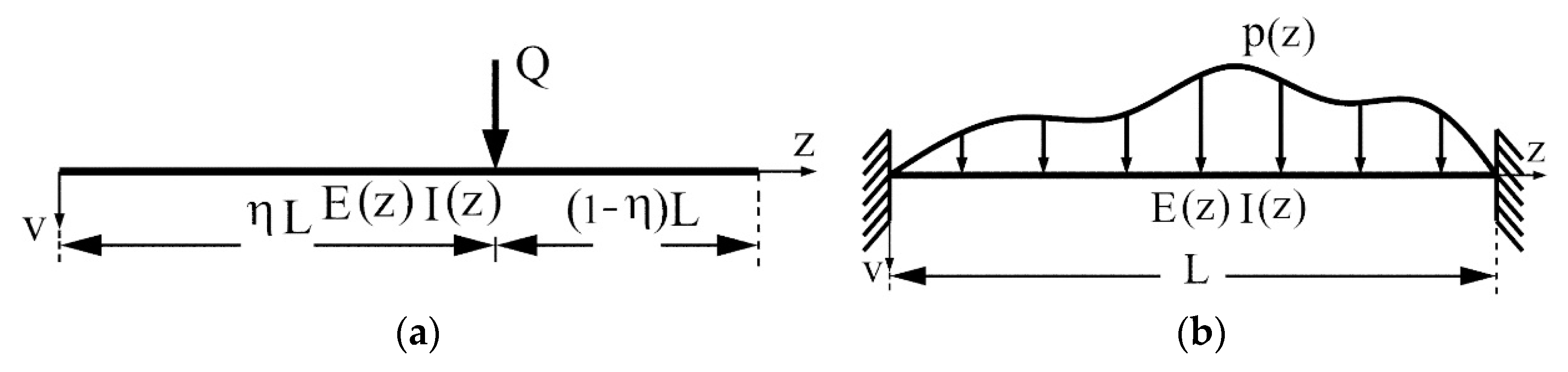
3.3. Beam Subjected to Singular Force

In this case, $p(z)$ = 0, Equation (4) can be written for both parts as follows (see Figure 2a).

$${\overrightarrow{y}}_1(z)=T\underset{˜}{M}(z).{\overrightarrow{y}}_0, 0\le z\le \eta L$$

(19)

$${\overrightarrow{y}}_2(z)=T\underset{˜}{M}(z).({\overrightarrow{y}}_1(\eta L)+\overrightarrow{\beta }), 0\le z\le (1-\eta )L$$

(20)

where $\overrightarrow{\beta }$ is

$$\overrightarrow{\beta }={\left(\begin{array}{cccc}0& 0& 0& -Q\end{array}\right)}^T$$

(21)

The unknowns of the problem can be written as follows.

$$\begin{array}{l}{v}_1(z)=M_0\left(-{\displaystyle {\int }_0^z\frac{z-\alpha }{E(\alpha )I(\alpha )}d\alpha }\right)-T_0\left({\displaystyle {\int }_0^z\frac{\alpha (z-\alpha )}{E(\alpha )I(\alpha )}}d\alpha \right)+v_0+{\phi }_{0}z\\ \end{array}$$

(22)

$$\begin{array}{l}{\phi }_1(z)=M_0\left(-{\displaystyle {\int }_0^z\frac{1}{E(\alpha )I(\alpha )}d\alpha }\right)-T_0\left({\displaystyle {\int }_0^z\frac{\alpha }{E(\alpha )I(\alpha )}}d\alpha \right)+{\phi }_0\\ \end{array}$$

(23)

$$M_1(z)=M_0+T_{o}z, T_1(z)=T_0$$

(24)

$$\begin{array}{l}{v}_2(z)=-M_0\left({\displaystyle {\int }_0^{\eta L}\frac{\eta L-\alpha }{E(\alpha )I(\alpha )}d\alpha }\right)-(\eta L{T}_0+M_0)\left({\displaystyle {\int }_0^z\frac{(z-\alpha )}{E(\alpha )I(\alpha )}}d\alpha \right)\\ +M_0(-z)\left({\displaystyle {\int }_0^{\eta L}\frac{1}{E(\alpha )I(\alpha )}d\alpha }\right)-T_0\left({\displaystyle {\int }_0^{\eta L}\frac{\alpha (\eta L-\alpha )}{E(\alpha )I(\alpha )}d\alpha }\right)\\ -T_{0}z\left({\displaystyle {\int }_0^{\eta L}\frac{\alpha }{E(\alpha )I(\alpha )}d\alpha }\right)+(Q-T_0)\left({\displaystyle {\int }_0^z\frac{\alpha (z-\alpha )}{E(\alpha )I(\alpha )}}d\alpha \right)+{\phi }_0(\eta L+z)+v_0\end{array}$$

(25)

$$\begin{array}{l}{\phi }_2(z)=M_0\left(-{\displaystyle {\int }_0^{\eta L}\frac{1}{E(\alpha )I(\alpha )}d\alpha }\right)-(\eta L{T}_0+M_0)\left({\displaystyle {\int }_0^z\frac{1}{E(\alpha )I(\alpha )}}d\alpha \right)\\ -T_0\left({\displaystyle {\int }_0^{\eta L}\frac{\alpha }{E(\alpha )I(\alpha )}d\alpha }\right)+(Q-T_0)\left({\displaystyle {\int }_0^z\frac{\alpha }{E(\alpha )I(\alpha )}}d\alpha \right)+{\phi }_0\end{array}$$

(26)

$$M_2(z)=T_o(\eta L+z)+M_0-Qz, T_2(z)=T_0-Q$$

(27)

4. Calculation of Fixed-End Moments

4.1. Fixed Beams with Both Ends Subjected to the Distributed Loads

The positive directions for the end moments are different in MIV and SDM (see Figure 3).

A fixed beam with both ends subjected to the distributed load is shown in Figure 2b. In this case, two of the initial values and end conditions can be written as

$$v_0=0, {\phi }_0=0 ; v(L)=0, \phi (L)=0$$

(28)

The other two initial values are found with the help of Equations (6) and (7) as follows.

$$\begin{array}{l}{M}_0=\left(\left({\displaystyle {\int }_0^L\frac{\alpha }{E(\alpha )I(\alpha )}d\alpha }\right)\times {\displaystyle {\int }_0^{L}p(\tau )}\left({\displaystyle {\int }_0^{L-\tau }-\frac{\alpha (\alpha -L+\tau )}{E(\alpha )I(\alpha )}d\alpha +\frac{{\gamma }^2(\tau -L)}{E(\tau )I(\tau )}}\right)\right. d\tau \\ \left.-\left({\displaystyle {\int }_0^L\frac{\alpha (L-\alpha )}{E(\alpha )I(\alpha )}d\alpha }\right)\times {\displaystyle {\int }_0^{L}p(\tau )}\left({\displaystyle {\int }_0^{L-\tau }\frac{\alpha }{E(\alpha )I(\alpha )}d\alpha -\frac{{\gamma }^2}{E(\tau )I(\tau )}}\right)d\tau \right)\\ /\left(\left({\displaystyle {\int }_0^L\frac{L-\alpha }{E(\alpha )I(\alpha )}d\alpha }\right)\right.\left.{\displaystyle {\int }_0^L\frac{\alpha }{E(\alpha )I(\alpha )}d\alpha }-\left({\displaystyle {\int }_0^L\frac{1}{E(\alpha )I(\alpha )}d\alpha }\right){\displaystyle {\int }_0^L\frac{\alpha (L-\alpha )}{E(\alpha )I(\alpha )}d\alpha }\right)\end{array}$$

(29)

$$\begin{array}{l}{T}_0=\left(\left({\displaystyle {\int }_0^L\frac{L-\alpha }{E(\alpha )I(\alpha )}d\alpha }\right){\displaystyle {\int }_0^{L}p(\tau )}\left({\displaystyle {\int }_0^{L-\tau }\frac{\alpha }{E(\alpha )I(\alpha )}d\alpha -\frac{{\gamma }^2}{E(\tau )I(\tau )}}\right)\right.d\tau \\ \left.-\left({\displaystyle {\int }_0^L\frac{1}{E(\alpha )I(\alpha )}d\alpha }\right)\times {\displaystyle {\int }_0^{L}p(\tau )}\left({\displaystyle {\int }_0^{L-\tau }-\frac{\alpha (\alpha -L+\tau )}{E(\alpha )I(\alpha )}d\alpha +\frac{{\gamma }^2(\tau -L)}{E(\tau )I(\tau )}}\right)d\tau \right)\\ /\left(\left({\displaystyle {\int }_0^L\frac{L-\alpha }{E(\alpha )I(\alpha )}d\alpha }\right)\right.\left.{\displaystyle {\int }_0^L\frac{\alpha }{E(\alpha )I(\alpha )}d\alpha }-\left({\displaystyle {\int }_0^L\frac{1}{E(\alpha )I(\alpha )}d\alpha }\right){\displaystyle {\int }_0^L\frac{\alpha (L-\alpha )}{E(\alpha )I(\alpha )}d\alpha }\right)\end{array}$$

(30)

Special cases

(a)

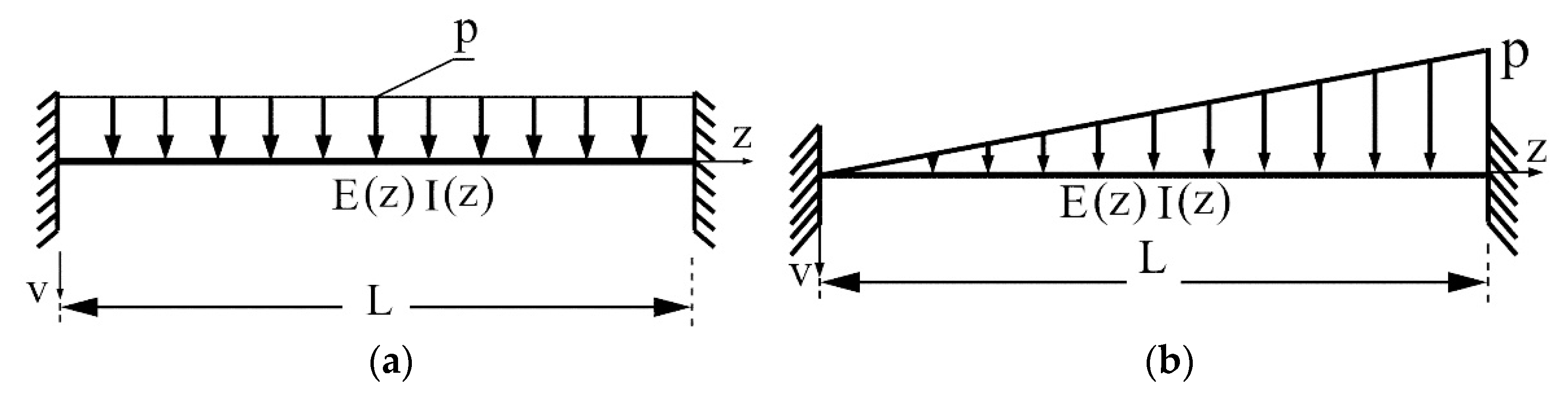
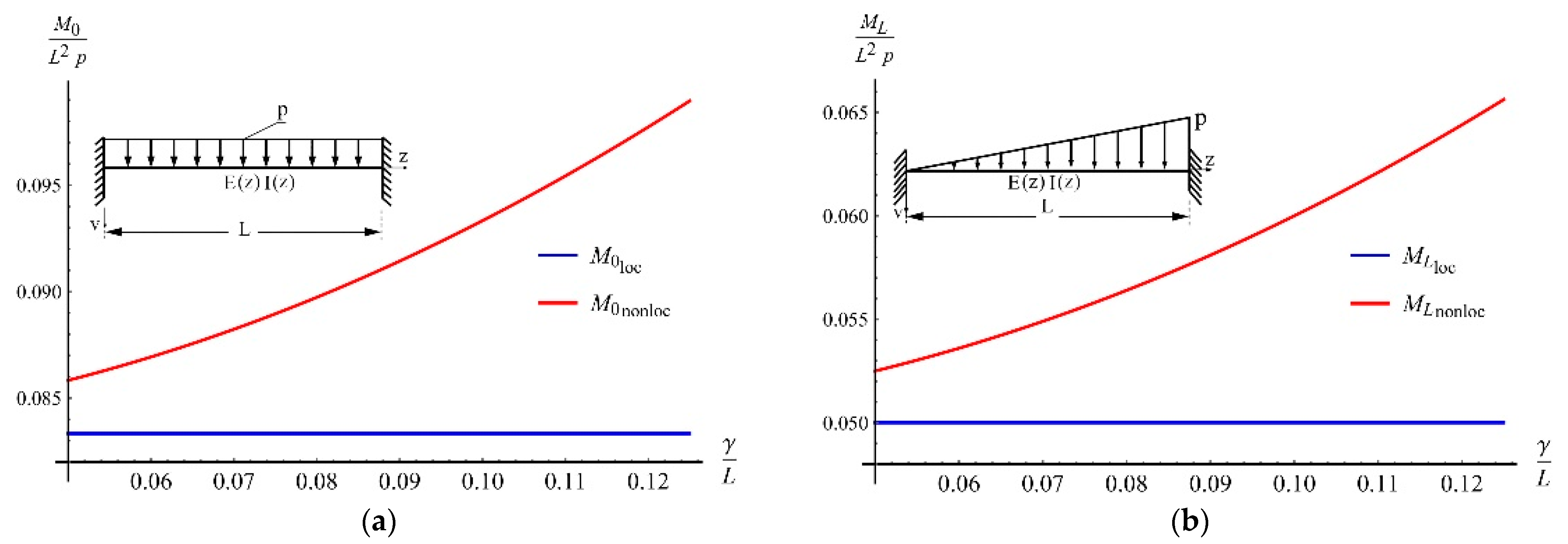
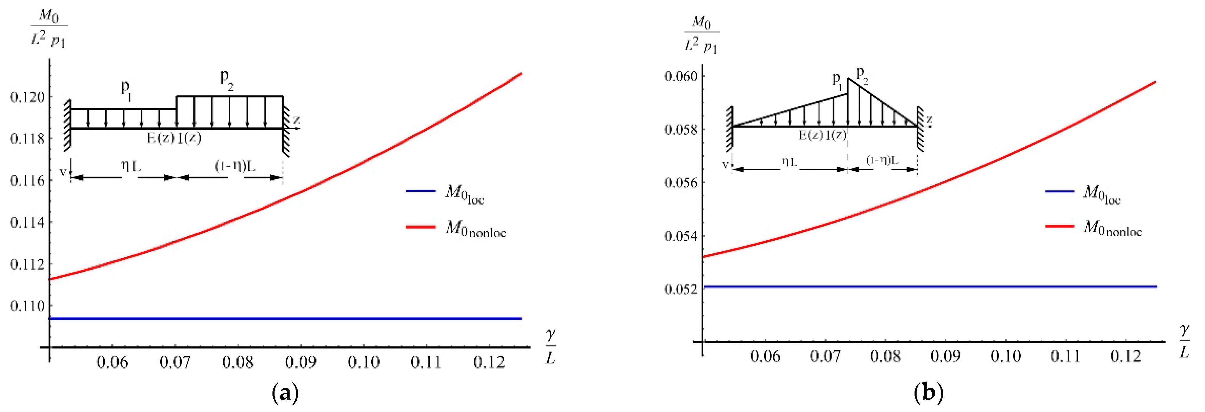
Uniform beam with constant cross section subjected to the uniform load (see Figure 4a).

In this case,

$$p(z)=p, E(z)=E, I(z)=I$$

(31)

Using Equations (29) and (30), the initial values M₀ and T₀ are found as follows.

$$M_0=-\frac{1}{12}p(12{\gamma }^2+L^2), T_0=\frac{Lp}{2}$$

(32)

The variation of the initial moment ($M_0$) in classical and nonlocal theory with respect to the $\gamma /L$ ratio is given in Figure 5a.

(b)

Uniform beam with a constant cross section subjected to the triangular load (see Figure 4b).

In this case,

$$p(z)=\frac{p}{L}z, E(z)=E, I(z)=I$$

(33)

Using Equations (29) and (30), the initial values $M_0$ and $T_0$ are found as follows.

$$M_0=-\frac{L^{2}p}{30}, T_0=\frac{3Lp}{20}-\frac{{\gamma }^{2}p}{L}$$

(34)

The end moments are found using Equation (8) as below.

$$M(L)=-\frac{1}{20}p(20{\gamma }^2+L^2), T(L)=-\frac{{\gamma }^{2}p}{L}-\frac{7Lp}{20}$$

(35)

The variation of the end moment ($M_L$) in classical and nonlocal theory with respect to the $\frac{\gamma }{L}$ ratio is given in Figure 5b.

4.2. Fixed Beams with Both Ends Subjected to the Different Distributed Loads

A fixed beam with both ends subjected to the two distributed loads is shown in Figure 6. In this case, the initial values and end conditions are

$$v_0=0, {\phi }_0=0 ; v_2((1-\eta )L)=0, {\phi }_2((1-\eta )L)=0$$

(36)

The other two initial values are found with the help of Equation (15) as follows.

$$\begin{array}{l}{M}_0=\left((\eta -1)L{\displaystyle {\int }_0^{\eta L}\frac{\alpha }{E(\alpha )I(\alpha )}d\alpha }\right.-{\displaystyle {\int }_0^{L-\eta L}-\frac{\alpha (\alpha +(\eta -1)L)}{E(\alpha )I(\alpha )}}d\alpha \\ -\eta L{\displaystyle {\int }_0^{L-\eta L}\frac{-\alpha -\eta L+L}{E(\alpha )I(\alpha )}}\left.d\alpha -{\displaystyle {\int }_0^{\eta L}\frac{\alpha (\eta L-\alpha )}{E(\alpha )I(\alpha )}d\alpha }\right)\\ \left({\displaystyle {\int }_0^{\eta L}{p}_1(\tau )}\left({\displaystyle {\int }_0^{\eta L-\tau }\frac{\alpha }{E(\alpha )I(\alpha )}d\alpha -\frac{{\gamma }^2}{E(\tau )I(\tau )}}\right)d\tau \right.\\ +{\displaystyle {\int }_0^{L-\eta L}{p}_2(\tau )}\left({\displaystyle {\int }_0^{-\eta L+L-\tau }\frac{\alpha }{E(\alpha )I(\alpha )}d\alpha -\frac{{\gamma }^2}{E(\tau )I(\tau )}}\right)d\tau \\ +{\displaystyle {\int }_0^{\eta L}-p_1(\tau )d\tau }\left(-{\displaystyle {\int }_0^{L-\eta L}\frac{\alpha }{E(\alpha )I(\alpha )}}d\alpha \right)-\left.{\displaystyle {\int }_0^{\eta L}{p}_1(\tau )}(\tau -\eta L)d\tau \left({\displaystyle {\int }_0^{L-\eta L}\frac{1}{E(\alpha )I(\alpha )}d\alpha }\right)\right)\\ -\left(\eta (-L){\displaystyle {\int }_0^{L-\eta L}\frac{1}{E(\alpha )I(\alpha )}d\alpha }-{\displaystyle {\int }_0^{\eta L}\frac{\alpha }{E(\alpha )I(\alpha )}d\alpha }-{\displaystyle {\int }_0^{L-\eta L}\frac{\alpha }{E(\alpha )I(\alpha )}d\alpha }\right)\\ \left(-(\eta -1)L{\displaystyle {\int }_0^{\eta L}{p}_1(\tau )}\right.\left({\displaystyle {\int }_0^{\eta L-\tau }\frac{\alpha }{E(\alpha )I(\alpha )}d\alpha -\frac{{\gamma }^2}{E(\tau )I(\tau )}}\right)d\tau \\ +{\displaystyle {\int }_0^{\eta L}\frac{p_1(\tau )\left(E(\tau )I(\tau ){\displaystyle {\int }_0^{\eta L-\tau }-\frac{\alpha (\alpha -\eta L+\tau )}{E(\alpha )I(\alpha )}d\alpha +{\gamma }^2(\tau -\eta L)}\right)}{E(\tau )I(\tau )}}d\tau \\ +{\displaystyle {\int }_0^{L-\eta L}\frac{p_2(\tau )\left(E(\tau )I(\tau ){\displaystyle {\int }_0^{-\eta L+L-\tau }-\frac{\alpha (\alpha +(\eta -1)L+\tau )}{E(\alpha )I(\alpha )}d\alpha +{\gamma }^2((\eta -1)L+\tau )}\right)}{E(\tau )I(\tau )}}d\tau \\ +{\displaystyle {\int }_0^{\eta L}-p_1(\tau )} d\tau \left(-{\displaystyle {\int }_0^{L-\eta L}-\frac{\alpha (\alpha +(\eta -1)L)}{E(\alpha )I(\alpha )}}d\alpha \right)-{\displaystyle {\int }_0^{\eta L}{p}_1(\tau )}\left. (\tau -\eta L) d\tau \left({\displaystyle {\int }_0^{L-\eta L}\frac{-\alpha -\eta L+L}{E(\alpha )I(\alpha )}}d\alpha \right)\right)\\ /\left(\eta (-L){\displaystyle {\int }_0^{L-\eta L}\frac{1}{E(\alpha )I(\alpha )}d\alpha }-\right.\left.{\displaystyle {\int }_0^{\eta L}\frac{\alpha }{E(\alpha )I(\alpha )}d\alpha }-{\displaystyle {\int }_0^{L-\eta L}\frac{\alpha }{E(\alpha )I(\alpha )}}d\alpha \right)\\ \left((\eta -1)L{\displaystyle {\int }_0^{\eta L}\frac{1}{E(\alpha )I(\alpha )}d\alpha }-{\displaystyle {\int }_0^{L-\eta L}\frac{-\alpha -\eta L+L}{E(\alpha )I(\alpha )}}d\alpha -{\displaystyle {\int }_0^{\eta L}\frac{\eta L-\alpha }{E(\alpha )I(\alpha )}d\alpha }\right)\\ -\left(-{\displaystyle {\int }_0^{\eta L}\frac{1}{E(\alpha )I(\alpha )}d\alpha }-{\displaystyle {\int }_0^{L-\eta L}\frac{1}{E(\alpha )I(\alpha )}}d\alpha \right)\left((\eta -1)L{\displaystyle {\int }_0^{\eta L}\frac{\alpha }{E(\alpha )I(\alpha )}d\alpha }\right.\\ -{\displaystyle {\int }_0^{L-\eta L}-\frac{\alpha (\alpha +(\eta -1)L)}{E(\alpha )I(\alpha )}}d\alpha -\eta L{\displaystyle {\int }_0^{L-\eta L}\frac{-\alpha -\eta L+L}{E(\alpha )I(\alpha )}}\left.d\alpha -{\displaystyle {\int }_0^{\eta L}\frac{\alpha (\eta L-\alpha )}{E(\alpha )I(\alpha )}d\alpha }\right)\end{array}$$

(37)

$$\begin{gathered} \begin{array}{l}{T}_0=-\left({\displaystyle {\int }_0^{L-\eta L}\frac{-\alpha -\eta L+L}{E(\alpha )I(\alpha )}}d\alpha +{\displaystyle {\int }_0^{\eta L}\frac{\eta L-\alpha }{E(\alpha )I(\alpha )}d\alpha }\right)\left(\left({\displaystyle {\int }_0^{L-\eta L}\frac{\alpha }{E(\alpha )I(\alpha )}}d\alpha \right)\right.\\ {\displaystyle {\int }_0^{\eta L}-p_1(\tau )} d\tau -{\displaystyle {\int }_0^{\eta L}\left({\displaystyle {\int }_0^{\eta L-\tau }\frac{\alpha }{E(\alpha )I(\alpha )}d\alpha -\frac{{\gamma }^2}{E(\tau )I(\tau )}}\right)}{p}_1(\tau )d\tau \\ -\left.{\displaystyle {\int }_0^{L-\eta L}\left({\displaystyle {\int }_0^{-\eta L+L-\tau }\frac{\alpha }{E(\alpha )I(\alpha )}d\alpha -\frac{{\gamma }^2}{E(\tau )I(\tau )}}\right) p_2(\tau )d\tau }\right)+\left({\displaystyle {\int }_0^{L-\eta L}\frac{1}{E(\alpha )I(\alpha )}}d\alpha \right)\\ \left(\left({\displaystyle {\int }_0^{L-\eta L}\frac{-\alpha (\alpha +L(\eta -1))}{E(\alpha )I(\alpha )}}d\alpha \right)\right.{\displaystyle {\int }_0^{\eta L}-p_1(\tau )} d\tau -\left({\displaystyle {\int }_0^{\eta L}\frac{\eta L-\alpha }{E(\alpha )I(\alpha )}d\alpha }\right)\\ {\displaystyle {\int }_0^{\eta L}(\tau -}\eta L)p_1(\tau )d\tau +L(\eta -1) {\displaystyle {\int }_0^{\eta L}\left({\displaystyle {\int }_0^{\eta L-\tau }\frac{\alpha }{E(\alpha )I(\alpha )}d\alpha -\frac{{\gamma }^2}{E(\tau )I(\tau )}}\right)} p_1(\tau )d\tau \\ -{\displaystyle {\int }_0^{\eta L}\frac{\left((\tau \right.-\eta L){\gamma }^2+E(\tau )I(\tau ){\displaystyle {\int }_0^{\eta L-\tau }-\frac{\alpha (\alpha -\eta L+\tau )}{E(\alpha )I(\alpha )}\left.d\alpha \right)p_1(\tau )}}{E(\tau )I(\tau )} }d\tau \\ -{\displaystyle {\int }_0^{L-\eta L}\frac{\left(L(\eta -1)+\tau ){\gamma }^2+E(\tau )I(\tau ){\displaystyle {\int }_0^{-\eta L+L-\tau }-\frac{\alpha (\alpha +L(\eta -1)+\tau )}{E(\alpha )I(\alpha )}d\alpha }\right)p_2(\tau )}{E(\tau )I(\tau )}}d\tau \\ +\left({\displaystyle {\int }_0^{\eta L}\frac{1}{E(\alpha )I(\alpha )}d\alpha }\right) \left(L(\eta -1) \left({\displaystyle {\int }_0^{L-\eta L}\frac{\alpha }{E(\alpha )I(\alpha )}d\alpha }\right) {\displaystyle {\int }_0^{\eta L}-p_1(\tau )} d\tau \right.\\ +\left({\displaystyle {\int }_0^{L-\eta L}\frac{-\alpha (\alpha +L(\eta -1))}{E(\alpha )I(\alpha )}}d\alpha \right) {\displaystyle {\int }_0^{\eta L}-p_1(\tau )} d\tau +\left(L(\eta -1) {\displaystyle {\int }_0^{L-\eta L}\frac{1}{E(\alpha )I(\alpha )}d\alpha }\right.\\ \left.+{\displaystyle {\int }_0^{L-\eta L}\frac{-\alpha -\eta L+L}{E(\alpha )I(\alpha )}}d\alpha \right) {\displaystyle {\int }_0^{\eta L}(\tau -}\eta L)p_1(\tau )d\tau \\ -{\displaystyle {\int }_0^{\eta L}\frac{\left((\tau \right.-\eta L){\gamma }^2+E(\tau )I(\tau ){\displaystyle {\int }_0^{\eta L-\tau }-\frac{\alpha (\alpha -\eta L+\tau )}{E(\alpha )I(\alpha )}\left.d\alpha \right)p_1(\tau )}}{E(\tau )I(\tau )} }d\tau \\ -L(\eta -1) {\displaystyle {\int }_0^{L-\eta L}\left({\displaystyle {\int }_0^{-\eta L+L-\tau }\frac{\alpha }{E(\alpha )I(\alpha )}d\alpha -\frac{{\gamma }^2}{E(\tau )I(\tau )}}\right) p_2(\tau )d\tau }\\ -\left.{\displaystyle {\int }_0^{L-\eta L}\frac{(L(\eta -1)+\tau ){\gamma }^2+E(\tau )I(\tau ){\displaystyle {\int }_0^{-\eta L+L-\tau }-\frac{\alpha (\alpha +L(\eta -1)+\tau )}{E(\alpha )I(\alpha )}\left.d\alpha \right)p_2(\tau )}}{E(\tau )I(\tau )}d\tau }\right)\end{array} \\ \begin{array}{l}/\left({\displaystyle {\int }_0^{\eta L}\frac{\alpha }{E(\alpha )I(\alpha )}}d\alpha +{\displaystyle {\int }_0^{L-\eta L}\frac{\alpha }{E(\alpha )I(\alpha )}}d\alpha \right)\hspace{0.17em}\hspace{0.17em}\left({\displaystyle {\int }_0^{L-\eta L}\frac{-\alpha -\eta L+L}{E(\alpha )I(\alpha )}}\right.d\alpha \\ +\left.{\displaystyle {\int }_0^{\eta L}\frac{\eta L-\alpha }{E(\alpha )I(\alpha )}d\alpha }\right)+\left({\displaystyle {\int }_0^{L-\eta L}\frac{1}{E(\alpha )I(\alpha )}d\alpha }\right)\hspace{0.17em}\hspace{0.17em}\left(L(\eta -1)\hspace{0.17em}{\displaystyle {\int }_0^{\eta L}\frac{\alpha }{E(\alpha )I(\alpha )}d\alpha }\right.\\ -{\displaystyle {\int }_0^{L-\eta L}\frac{-\alpha (\alpha +L(\eta -1))}{E(\alpha )I(\alpha )}}d\alpha +\eta L\hspace{0.17em}{\displaystyle {\int }_0^{\eta L}\frac{\eta L-\alpha }{E(\alpha )I(\alpha )}d\alpha }\\ -\left.{\displaystyle {\int }_0^{\eta L}\frac{\alpha (\eta L-\alpha )}{E(\alpha )I(\alpha )}d\alpha }\right)-\left({\displaystyle {\int }_0^{\eta L}\frac{1}{E(\alpha )I(\alpha )}d\alpha }\right)\hspace{0.17em}\hspace{0.17em}\left(L(\eta -1)\hspace{0.17em}\left(\eta L\hspace{0.17em}{\displaystyle {\int }_0^{L-\eta L}\frac{1}{E(\alpha )I(\alpha )}d\alpha }\right.\right.\\ +\left.{\displaystyle {\int }_0^{L-\eta L}\frac{\alpha }{E(\alpha )I(\alpha )}}d\alpha \right)+{\displaystyle {\int }_0^{L-\eta L}\frac{-\alpha (\alpha +L(\eta -1))}{E(\alpha )I(\alpha )}}d\alpha \\ +\eta L\hspace{0.17em}\left.{\displaystyle {\int }_0^{L-\eta L}\frac{-\alpha -\eta L+L}{E(\alpha )I(\alpha )}}d\alpha +{\displaystyle {\int }_0^{\eta L}\frac{\alpha (\eta L-\alpha )}{E(\alpha )I(\alpha )}d\alpha }\right)\end{array} \end{gathered}$$

(38)

Special cases: A uniform beam subjected to different types of loads.

(a)

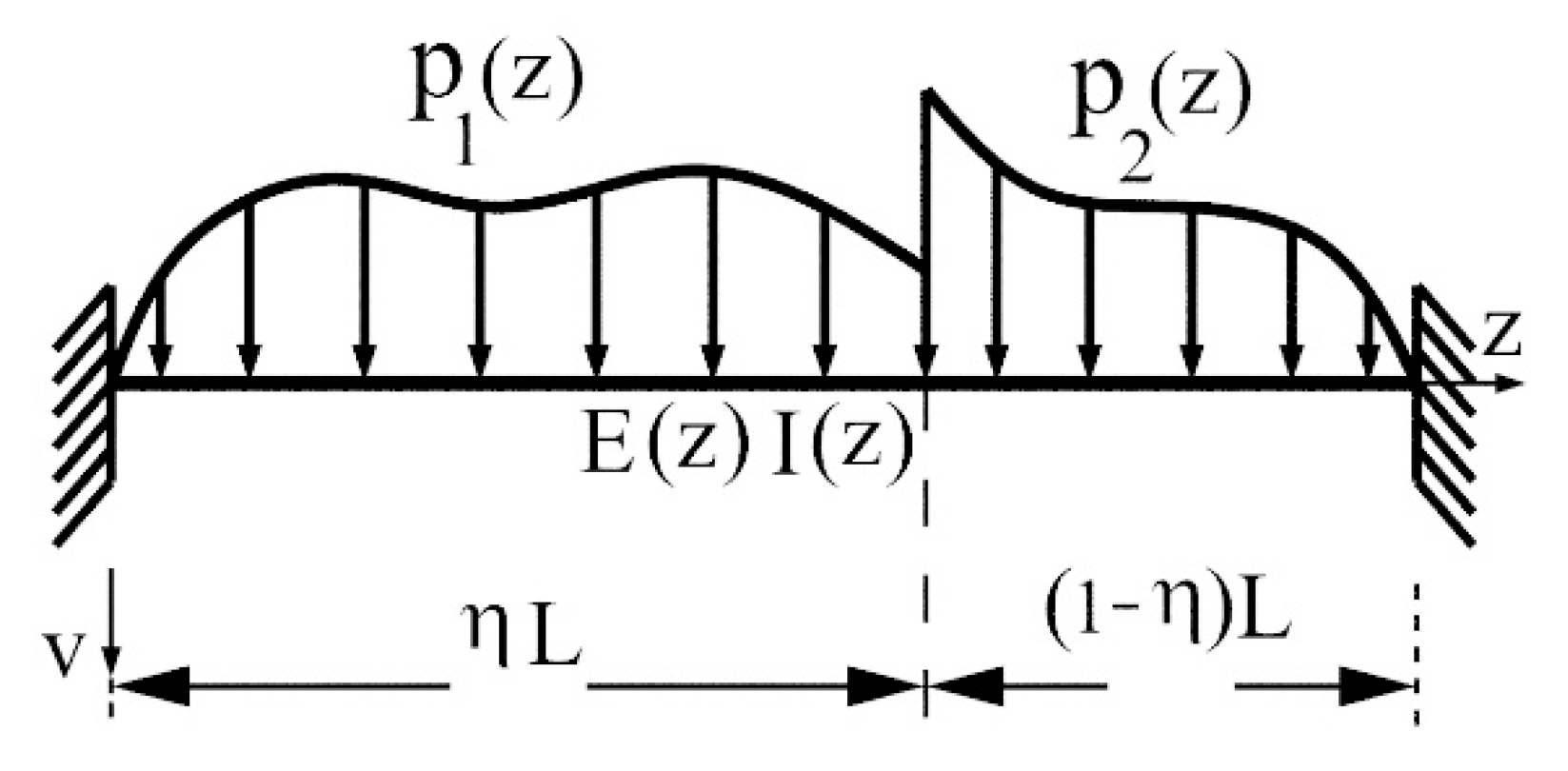
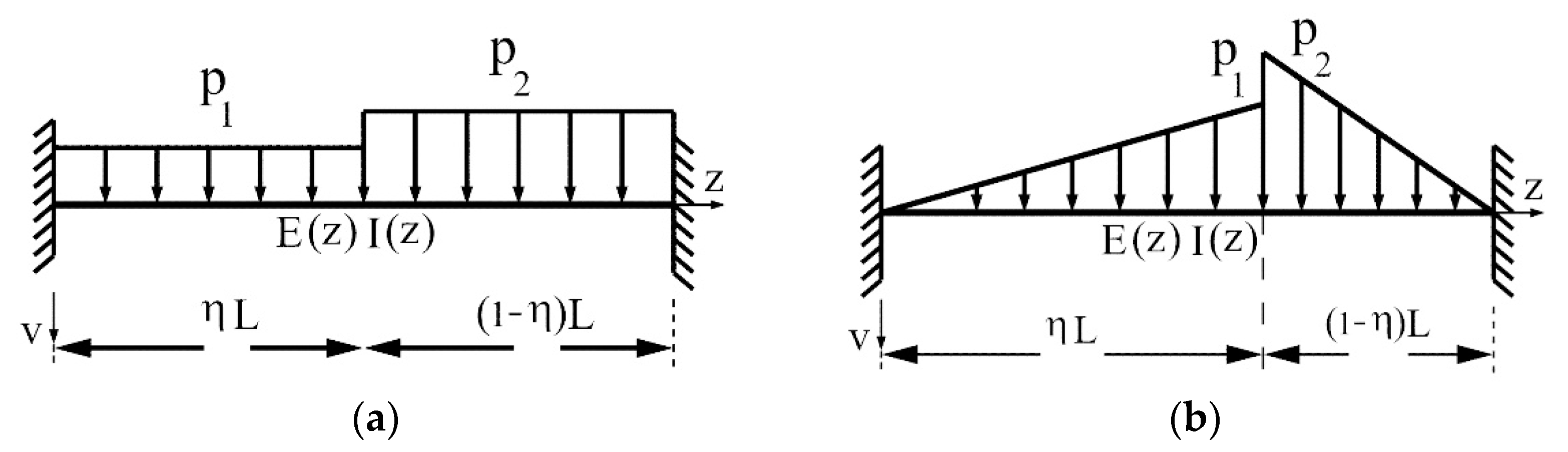
Uniform beam with a constant cross section subjected to two different uniform loads (see Figure 7a).

For $\eta =\frac{1}{2}$ and

$$\begin{array}{l}{p}_1(z)=p_1 , 0<z<\eta L\\ p_2(z)=p_2 , 0<z<(1-\eta )L\end{array}$$

(39)

$M_0$ and $M_2(L/2)$ are obtained using Equations (17) and (37) as follows.

$$M_0=\frac{1}{192}\left(p_2(4\right.8{\gamma }^2-5L^2)-p_1(240{\gamma }^2+11\left.L^2)\right)$$

$$M_2(L/2)=\frac{1}{192}\left(p_1(4\right.8{\gamma }^2-5L^2)-p_2(240{\gamma }^2+11\left.L^2)\right)$$

(40)

$T_0$ and $T_2(L/2)$ are found using Equations (18) and (38) as below.

$$T_0=\frac{p_1(48{\gamma }^2+13L^2)+3p_2(L^2-16{\gamma }^2)}{32L}, T_2(L/2)=-\frac{3p_1(L^2-16{\gamma }^2)+p_2(48{\gamma }^2+13L^2)}{32L}$$

(41)

The variation of the initial moment ($M_0$) in classical and nonlocal theory with respect to the $\gamma /L$ ratio is given in Figure 8a.

(b)

Uniform beam with a constant cross section subjected to the two different triangular loads (see Figure 7b).

For $\eta =\frac{1}{2}$,

$$\begin{array}{l}{p}_1(z)=\frac{2p_{1}z}{L} , 0<z<\eta L\\ p_2(z)=p_2-\frac{2p_{2}z}{L} , 0<z<(1-\eta )L\\ \end{array}$$

(42)

$M_0$ and $M_2(L/2)$ are obtained using Equations (17) and (37) as follows.

$$M_0=\frac{1}{480}\left(-16\right.p_1(15{\gamma }^2+L^2)-9L^2\left.p_2\right)$$

(43)

$$M_2(L/2)=\frac{1}{480}\left(-16\right.p_2(15{\gamma }^2+L^2)-9L^2\left.p_1\right)$$

(44)

$T_0$ and $T_2(L/2)$ are found using Equations (18) and (38) as below.

$$\begin{gathered} T_0=\frac{p_1(80{\gamma }^2+29L^2)+p_2(11L^2-80{\gamma }^2)}{160L} \\ {T}_2(L/2)=\frac{p_1(80{\gamma }^2-11L^2)-p_2(80{\gamma }^2+29L^2)}{160L} \end{gathered}$$

(45)

The variation of the initial moment ($M_0$) in classical and nonlocal theory with respect to the $\gamma /L$ ratio is given in Figure 8b.

4.3. Beams Subjected to Singular Force

4.3.1. Fixed Beam with Both Ends Subjected to Singular Forces

In this case (see Figure 9a), two of the initial values and end conditions are

$$v_0=0, {\phi }_0=0 ; v_2((1-\eta )L)=0, {\phi }_2((1-\eta )L)=0$$

(46)

Two other initial values ($M_0$ and $T_0$) are obtained using Equations (25) and (26) as follows.

$$\begin{array}{l}{M}_0=\left(-Q\hspace{0.17em}\left(\eta (-L)\hspace{0.17em}\left({\displaystyle {\int }_0^{L-\eta L}\frac{1}{E(\alpha )I(\alpha )}}d\alpha \right)\right.\hspace{0.17em}{\displaystyle {\int }_0^{L-\eta L}-\frac{\alpha (\alpha +(\eta -1)L)}{E(\alpha )I(\alpha )}}d\alpha \right.\\ -\left({\displaystyle {\int }_0^{\eta L}\frac{\alpha }{E(\alpha )I(\alpha )}d\alpha }\right)\times \left((\eta -1)L{\displaystyle {\int }_0^{L-\eta L}\frac{\alpha }{E(\alpha )I(\alpha )}d\alpha }+{\displaystyle {\int }_0^{L-\eta L}-\frac{\alpha (\alpha +(\eta -1)L)}{E(\alpha )I(\alpha )}}d\alpha \right)\\ \left.\left.+\left({\displaystyle {\int }_0^{L-\eta L}\frac{\alpha }{E(\alpha )I(\alpha )}d\alpha }\right)\times \left(\eta L{\displaystyle {\int }_0^{L-\eta L}\frac{-\alpha -\eta L+L}{E(\alpha )I(\alpha )}}\right.d\alpha +{\displaystyle {\int }_0^{\eta L}\left.\frac{\alpha (\eta L-\alpha )}{E(\alpha )I(\alpha )}d\alpha \right)}\right)\right)\\ /\left(\left(\eta (-L){\displaystyle {\int }_0^{L-\eta L}\frac{1}{E(\alpha )I(\alpha )}d\alpha }\right.\right.-{\displaystyle {\int }_0^{\eta L}\frac{\alpha }{E(\alpha )I(\alpha )}d\alpha }-\left.{\displaystyle {\int }_0^{L-\eta L}\frac{\alpha }{E(\alpha )I(\alpha )}d\alpha }\right)\\ \times \left((\eta -1)L{\displaystyle {\int }_0^{\eta L}\frac{1}{E(\alpha )I(\alpha )}d\alpha }\right.-{\displaystyle {\int }_0^{L-\eta L}\frac{-\alpha -\eta L+L}{E(\alpha )I(\alpha )}}\left.\hspace{0.17em}d\alpha -{\displaystyle {\int }_0^{\eta L}\frac{\eta L-\alpha }{E(\alpha )I(\alpha )}d\alpha }\right)\\ -\left(-{\displaystyle {\int }_0^{\eta L}\frac{1}{E(\alpha )I(\alpha )}d\alpha -}\right.\left.{\displaystyle {\int }_0^{L-\eta L}\frac{1}{E(\alpha )I(\alpha )}d\alpha }\right)\\ \times \left((\eta -1)L{\displaystyle {\int }_0^{\eta L}\frac{\alpha }{E(\alpha )I(\alpha )}d\alpha }\right.-{\displaystyle {\int }_0^{L-\eta L}-\frac{\alpha (\alpha +(\eta -1)L)}{E(\alpha )I(\alpha )}}d\alpha \\ -\eta L{\displaystyle {\int }_0^{L-\eta L}\frac{-\alpha -\eta L+L}{E(\alpha )I(\alpha )}}\left.\hspace{0.17em}d\alpha -{\displaystyle {\int }_0^{\eta L}\left.\frac{\alpha (\eta L-\alpha )}{E(\alpha )I(\alpha )}d\alpha \right)}\right)\end{array}$$

(47)

$$\begin{array}{l}{T}_0=Q\hspace{0.17em}\left(\left(\hspace{0.17em}\left.{\displaystyle {\int }_0^{L-\eta L}\frac{1}{E(\alpha )I(\alpha )}}d\alpha \right)\right.\hspace{0.17em}{\displaystyle {\int }_0^{L-\eta L}-\frac{\alpha (\alpha +(\eta -1)L)}{E(\alpha )I(\alpha )}}d\alpha \right.\\ +\left({\displaystyle {\int }_0^{\eta L}\frac{1}{E(\alpha )I(\alpha )}d\alpha }\right)\left((\eta -1)L{\displaystyle {\int }_0^{L-\eta L}\frac{\alpha }{E(\alpha )I(\alpha )}d\alpha }+{\displaystyle {\int }_0^{L-\eta L}-\frac{\alpha (\alpha +(\eta -1)L)}{E(\alpha )I(\alpha )}}d\alpha \right)\\ -\left({\displaystyle {\int }_0^{L-\eta L}\frac{\alpha }{E(\alpha )I(\alpha )}d\alpha }\right)\times \left({\displaystyle {\int }_0^{L-\eta L}\frac{-\alpha -\eta L+L}{E(\alpha )I(\alpha )}}\right.d\alpha +\left.{\displaystyle {\int }_0^{\eta L}\left.\frac{\eta L-\alpha }{E(\alpha )I(\alpha )}d\alpha \right)}\right)\\ /\left(-\left({\displaystyle {\int }_0^{\eta L}\frac{\alpha }{E(\alpha )I(\alpha )}d\alpha }\right.\right.+\left.{\displaystyle {\int }_0^{L-\eta L}\frac{\alpha }{E(\alpha )I(\alpha )}d\alpha }\right)\\ \times \left({\displaystyle {\int }_0^{L-\eta L}\frac{-\alpha -\eta L+L}{E(\alpha )I(\alpha )}}\right.\left.\hspace{0.17em}d\alpha +{\displaystyle {\int }_0^{\eta L}\frac{\eta L-\alpha }{E(\alpha )I(\alpha )}d\alpha }\right)\\ +\left({\displaystyle {\int }_0^{\eta L}\frac{1}{E(\alpha )I(\alpha )}d\alpha }\right)\hspace{0.17em}\left((\eta -1)L\hspace{0.17em}\left(\eta L{\displaystyle {\int }_0^{L-\eta L}\frac{1}{E(\alpha )I(\alpha )}d\alpha }\right.\right.+\left.{\displaystyle {\int }_0^{L-\eta L}\frac{\alpha }{E(\alpha )I(\alpha )}d\alpha }\right)\\ {\displaystyle {\int }_0^{L-\eta L}-\frac{\alpha (\alpha +(\eta -1)L)}{E(\alpha )I(\alpha )}}d\alpha \\ +\eta L{\displaystyle {\int }_0^{L-\eta L}\frac{-\alpha -\eta L+L}{E(\alpha )I(\alpha )}}\hspace{0.17em}d\alpha \left.+{\displaystyle {\int }_0^{\eta L}\frac{\alpha (\eta L-\alpha )}{E(\alpha )I(\alpha )}d\alpha }\right)\\ +\left({\displaystyle {\int }_0^{L-\eta L}\frac{1}{E(\alpha )I(\alpha )}}d\alpha \right)\hspace{0.17em}\left((\eta -1)(-L){\displaystyle {\int }_0^{\eta L}\frac{\alpha }{E(\alpha )I(\alpha )}d\alpha }\right.\\ +{\displaystyle {\int }_0^{L-\eta L}-\frac{\alpha (\alpha +(\eta -1)L)}{E(\alpha )I(\alpha )}}d\alpha -\eta L{\displaystyle {\int }_0^{\eta L}\frac{\eta L-\alpha }{E(\alpha )I(\alpha )}\hspace{0.17em}d\alpha }\\ +\left.\left.{\displaystyle {\int }_0^{\eta L}\frac{\alpha (\eta L-\alpha )}{E(\alpha )I(\alpha )}d\alpha }\right)\right)\end{array}$$

(48)

Special Case: E and I are constant.

For $E(z)=E$ and $I(z)=I$, $M_0$ and $T_0$ are found with the help of Equations (47) and (48) as follows.

$$M_0={(\eta -1)}^2\eta (-L)Q, T_0={(\eta -1)}^2(2\eta +1) Q$$

(49)

4.3.2. Fixed-Pinned Beams

In this case, two of the initial values are (see Figure 9b)

$$v_0=0, {\phi }_0=0$$

(50)

The end conditions are

$$v_2((1-\eta )L)=0, M_2((1-\eta )L)=0$$

(51)

$M_0$ and $T_0$ are obtained using Equations (25) and (26) as below.

$$\begin{array}{l}{M}_0=\left(LQ \left({(\eta -1)}^{2}L) \left({\displaystyle {\int }_0^{\eta L}\frac{\alpha }{E(\alpha )I(\alpha )}d\alpha }\right)\right. \right.\\ -(\eta -1) \left(\eta L {\displaystyle {\int }_0^{L-\eta L}\frac{-\alpha -\eta L+L}{E(\alpha )I(\alpha )}}\right. d\alpha +\left.{\displaystyle {\int }_0^{\eta L}\frac{\alpha (\eta L-\alpha )}{E(\alpha )I(\alpha )}d\alpha }\right)\\ -\eta \left.\left.{\displaystyle {\int }_0^{L-\eta L}-\frac{\alpha (\alpha +(\eta -1)L)}{E(\alpha )I(\alpha )}}d\alpha \right)\right)\\ / \left({\displaystyle {\int }_0^{L-\eta L}-\frac{\alpha (\alpha +(\eta -1)L)}{E(\alpha )I(\alpha )}}d\alpha \right.\\ + (\eta -1)L\left(L{\displaystyle {\int }_0^{\eta L}\frac{1}{E(\alpha )I(\alpha )}d\alpha }\right.-{\displaystyle {\int }_0^{\eta L}\frac{\alpha }{E(\alpha )I(\alpha )}d\alpha }\\ +\left.{\displaystyle {\int }_0^{L-\eta L}\frac{-\alpha -\eta L+L}{E(\alpha )I(\alpha )}} d\alpha \right)-L {\displaystyle {\int }_0^{\eta L}\frac{\eta L-\alpha }{E(\alpha )I(\alpha )}d\alpha }+\left.{\displaystyle {\int }_0^{\eta L}\frac{\alpha (\eta L-\alpha )}{E(\alpha )I(\alpha )}d\alpha }\right)\end{array}$$

(52)

$$\begin{array}{l}{T}_0=Q \left({\displaystyle {\int }_0^{L-\eta L}-\frac{\alpha (\alpha +(\eta -1)L)}{E(\alpha )I(\alpha )}}d\alpha \right.\\ + (\eta -1)L \left((L-\eta L) {\displaystyle {\int }_0^{\eta L}\frac{1}{E(\alpha )I(\alpha )}d\alpha }\right.\\ +{\displaystyle {\int }_0^{L-\eta L}\frac{-\alpha -\eta L+L}{E(\alpha )I(\alpha )}} d\alpha +\left.\left.{\displaystyle {\int }_0^{\eta L}\frac{\eta L-\alpha }{E(\alpha )I(\alpha )}d\alpha }\right)\right)\\ / \left({\displaystyle {\int }_0^{L-\eta L}-\frac{\alpha (\alpha +(\eta -1)L)}{E(\alpha )I(\alpha )}}d\alpha \right.+ (\eta -1)L \left(L{\displaystyle {\int }_0^{\eta L}\frac{1}{E(\alpha )I(\alpha )}d\alpha }\right.\\ -{\displaystyle {\int }_0^{\eta L}\frac{\alpha }{E(\alpha )I(\alpha )}d\alpha }+\left.{\displaystyle {\int }_0^{L-\eta L}\frac{-\alpha -\eta L+L}{E(\alpha )I(\alpha )}} d\alpha \right)\\ -L {\displaystyle {\int }_0^{\eta L}\frac{\eta L-\alpha }{E(\alpha )I(\alpha )}d\alpha }+\left.{\displaystyle {\int }_0^{\eta L}\frac{\alpha (\eta L-\alpha )}{E(\alpha )I(\alpha )}d\alpha }\right)\end{array}$$

(53)

Special Case: E and I are constant.

For $E(z)=E$ and $I(z)=I$, $M_0$ and $T_0$ are found with the help of Equations (52) and (53) as follows.

$$M_0=-\frac{1}{2}(\eta -2) (\eta -1)\eta LQ, T_0=\frac{1}{2}\left((\eta -3\right.) \left.{\eta }^2+2\right) Q$$

(54)

5. Calculation of Stiffness Factors

5.1. Calculating the Moment $\mu$ Corresponding to the Unit Rotation for the Figure 10a

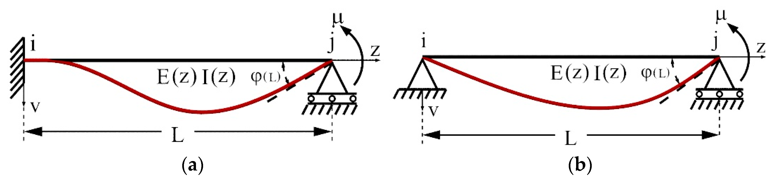
In this case, the applied moment $\mu$ rotates the end j by an amount $\phi (L)$. Two of the initial values are (see Figure 10a)

$$v_0=0, {\phi }_0=0$$

(55)

Figure 10. (a) The applied moment $\mu$ rotates the end j by an amount of $\phi (L)$; (b) the applied moment $\mu$ rotates the end j by an amount of $\phi (L)$.

Figure 10. (a) The applied moment $\mu$ rotates the end j by an amount of $\phi (L)$; (b) the applied moment $\mu$ rotates the end j by an amount of $\phi (L)$.

Using Equation (4), the unknowns can be written as

$$v(z)=M_0\left.\left(-{\displaystyle {\int }_0^z\frac{z-\alpha }{E(\alpha )I(\alpha )}}\right. d\alpha \right)-T_0\left.\left({\displaystyle {\int }_0^z\frac{\alpha (z-\alpha )}{E(\alpha )I(\alpha )}}\right. d\alpha \right)$$

(56)

$$\phi (z)=M_0\left.\left(-{\displaystyle {\int }_0^z\frac{1}{E(\alpha )I(\alpha )}}\right. d\alpha \right)-T_0\left.\left({\displaystyle {\int }_0^z\frac{\alpha }{E(\alpha )I(\alpha )}}\right. d\alpha \right)$$

(57)

$$\begin{array}{l}M(z)=M_0+T_{0}z\end{array}$$

(58)

$$T(z)=T_0$$

(59)

The end conditions are

$$v(L)=0, M(L)=\mu$$

(60)

The other initial values ($M_0, T_0$) are obtained using Equations (56) and (58) as follows.

$$M_0=\frac{\mu }{1-\frac{L {\displaystyle {\int }_0^L\frac{L-\alpha }{E(\alpha )I(\alpha )}d\alpha }}{{\displaystyle {\int }_0^L\frac{\alpha (L-\alpha )}{E(\alpha )I(\alpha )}d\alpha }}}, T_0=\frac{\mu }{L-\frac{{\displaystyle {\int }_0^L\frac{\alpha (L-\alpha )}{E(\alpha )I(\alpha )}d\alpha }}{{\displaystyle {\int }_0^L\frac{L-\alpha }{E(\alpha )I(\alpha )}d\alpha }}}$$

(61)

The moment $\mu$ is found with the help of $\phi (L)$ = −1 as below.

$$m_{j{\theta }_j}=\mu =\frac{{\displaystyle {\int }_0^L\frac{\alpha (L-\alpha )}{E(\alpha )I(\alpha )}d\alpha }-L {\displaystyle {\int }_0^L\frac{L-\alpha }{E(\alpha )I(\alpha )}d\alpha }}{\left({\displaystyle {\int }_0^L\frac{1}{E(\alpha )I(\alpha )}d\alpha }\right) {\displaystyle {\int }_0^L\frac{\alpha (L-\alpha )}{E(\alpha )I(\alpha )}d\alpha } -\left({\displaystyle {\int }_0^L\frac{L-\alpha }{E(\alpha )I(\alpha )}d\alpha }\right) {\displaystyle {\int }_0^L\frac{\alpha }{E(\alpha )I(\alpha )}d\alpha }}$$

(62)

Special case: E and I are constant.

For $E(z)=E, I(z)=I$,

$$m_{j {\theta }_j}=\frac{4EI}{L}, m_{i {\theta }_j}=-M_0=\frac{2EI}{L}, T_0=\frac{6EI}{L^2}, T(L)=\frac{6EI}{L^2}$$

(63)

5.2. Calculating the Moment $\mu$ Corresponding to the Unit Rotation for the Figure 10b

In this case, the applied moment $\mu$ rotates the end j by an amount $\phi (L)$. The initial values and end conditions are (see Figure 10b)

$$v_0=0, M_0=0 ; v(L)=0, M(L)=\mu$$

(64)

Using Equation (4), the unknowns can be written as

$$v(z)={\phi }_{0}z-T_0 \left.\left({\displaystyle {\int }_0^z\frac{\alpha (z-\alpha )}{E(\alpha )I(\alpha )}}\right. d\alpha \right); \phi (z)={\phi }_0-T_0 \left.\left({\displaystyle {\int }_0^z\frac{\alpha }{E(\alpha )I(\alpha )}}\right. d\alpha \right)$$

(65)

$$M(z)=T_{0}z , T(z)=T_0$$

(66)

The other initial values (${\phi }_0$, $T_0$) are obtained using Equation (66) as follows.

$${\phi }_0=\frac{\mu {\displaystyle {\int }_0^L\frac{\alpha (L-\alpha )}{E(\alpha )I(\alpha )}d\alpha }}{L^2}, T_0=\frac{\mu }{L}$$

(67)

The moment $\mu$ and $T_0$ are found with the help of $\phi (L)$ = −1 as below.

$$m_{j{\theta }_j}=\mu =\frac{L^2}{L {\displaystyle {\int }_0^L\frac{\alpha }{E(\alpha )I(\alpha )}d\alpha - {\displaystyle {\int }_0^L\frac{\alpha (L-\alpha )}{E(\alpha )I(\alpha )}d\alpha } }}$$

(68)

$$T_0=T(L)=\frac{L}{L {\displaystyle {\int }_0^L\frac{\alpha }{E(\alpha )I(\alpha )}d\alpha - {\displaystyle {\int }_0^L\frac{\alpha (L-\alpha )}{E(\alpha )I(\alpha )}d\alpha } }}$$

(69)

Special case: E and I are constant.

For $E(z)=E, I(z)=I$,

$$m_{j {\theta }_j}=\frac{3EI}{L}, T_0=\frac{3EI}{L^2}, T(L)=\frac{3EI}{L^2}$$

(70)

5.3. Calculating the Moment $\mu$ Corresponding to the Unit Deflection for the Figure 11a

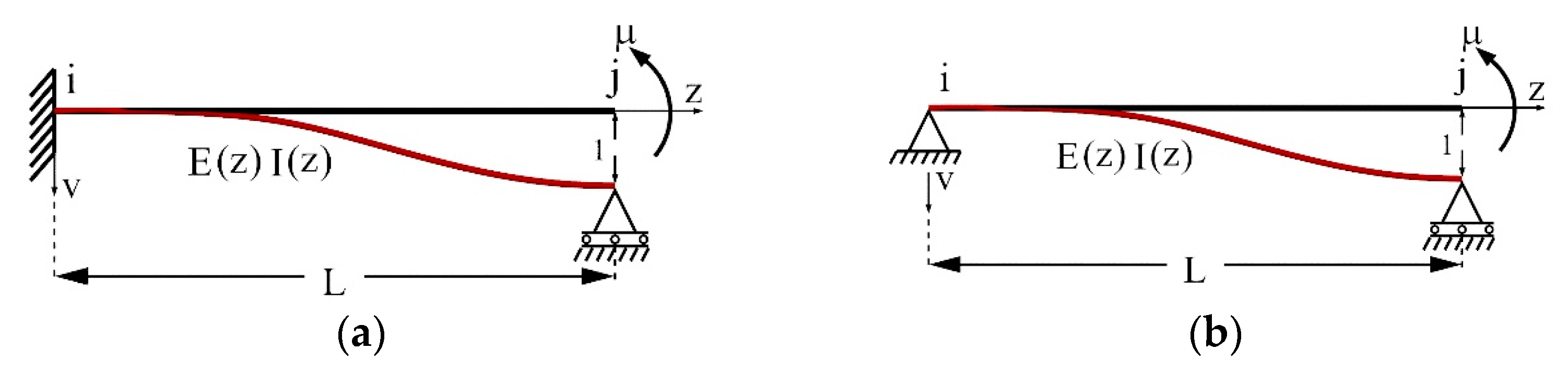
In this case, vertical displacement occurs at the j-end of the beam owing to the moment $\mu$. The initial values and end conditions are (see Figure 11a)

$$v_0=0, {\phi }_0=0 ; \phi (L)=0, M(L)=\mu$$

(71)

Figure 11. (a) Vertical displacement occurs at the j-end of the beam owing to the moment $\mu$; (b) vertical displacement occurs at the j-end of the beam owing to the moment $\mu$.

Figure 11. (a) Vertical displacement occurs at the j-end of the beam owing to the moment $\mu$; (b) vertical displacement occurs at the j-end of the beam owing to the moment $\mu$.

Using Equation (4), the unknowns can be written as

$$v(z)=M_0 \left.\left(-{\displaystyle {\int }_0^z\frac{z-\alpha }{E(\alpha )I(\alpha )}}\right. d\alpha \right)-T_0 \left.\left({\displaystyle {\int }_0^z\frac{\alpha (z-\alpha )}{E(\alpha )I(\alpha )}}\right. d\alpha \right)$$

(72)

$$\phi (z)=M_0 \left.\left(-{\displaystyle {\int }_0^z\frac{1}{E(\alpha )I(\alpha )}}\right. d\alpha \right)-T_0 \left.\left({\displaystyle {\int }_0^z\frac{\alpha }{E(\alpha )I(\alpha )}}\right. d\alpha \right)$$

(73)

$$M(z)=M_0+T_{0}z , T(z)=T_0$$

(74)

The other initial values ($M_0$, $T_0$) are obtained using Equations (73) and (74) as follows.

$$M_0=\frac{\mu }{1-\frac{L {\displaystyle {\int }_0^L\frac{1}{E(\alpha )I(\alpha )}d\alpha }}{{\displaystyle {\int }_0^L\frac{\alpha }{E(\alpha )I(\alpha )}d\alpha }}}, T_0=\frac{\mu }{L-\frac{{\displaystyle {\int }_0^L\frac{\alpha }{E(\alpha )I(\alpha )}d\alpha }}{{\displaystyle {\int }_0^L\frac{1}{E(\alpha )I(\alpha )}d\alpha }}}$$

(75)

The moment $\mu$ is found with the help of $v(L)$= 1 as below.

$$m_{j\delta }=\mu =\frac{\left({\displaystyle {\int }_0^L\frac{\alpha }{E(\alpha )I(\alpha )}d\alpha }-L {\displaystyle {\int }_0^L\frac{1}{E(\alpha )I(\alpha )}d\alpha }\right)}{\left(\left(\left.{\displaystyle {\int }_0^L\frac{1}{E(\alpha )I(\alpha )}d\alpha }\right)\right.\right. {\displaystyle {\int }_0^L\frac{\alpha (L-\alpha )}{E(\alpha )I(\alpha )}d\alpha }- \left({\displaystyle {\int }_0^L\frac{L-\alpha }{E(\alpha )I(\alpha )}d\alpha }\right) \left.{\displaystyle {\int }_0^L\frac{\alpha }{E(\alpha )I(\alpha )}d\alpha } \right)}$$

(76)

Special case: E and I are constant.

For $E(z)=E, I(z)=I$,

$$m_{j \delta }=-M_0=\frac{6EI}{L^2}, T_0=T(L)=\frac{12EI}{L^3}$$

(77)

5.4. Calculating the Moment $\mu$ Corresponding to the Unit Deflection for the Figure 11b

In this case, vertical displacement occurs at the j-end of the beam owing to the moment. The initial values and end conditions are (see Figure 11b)

$$v_0=0, M_0=0 , M(L)=\mu , \phi (L)=0$$

(78)

Using Equation (4), the unknowns can be written as

$$v(z)={\phi }_{0}z-T_0 \left.\left({\displaystyle {\int }_0^z\frac{\alpha (z-\alpha )}{E(\alpha )I(\alpha )}}\right. d\alpha \right), \phi (z)={\phi }_0-T_0 \left.\left({\displaystyle {\int }_0^z\frac{\alpha }{E(\alpha )I(\alpha )}}\right. d\alpha \right)$$

(79)

$$M(z)=T_{0}z , T(z)=T_0$$

(80)

The other initial values (${\phi }_0$, $T_0$) are obtained using Equation (80) as follows.

$${\phi }_0=\frac{\mu {\displaystyle {\int }_0^L\frac{\alpha }{E(\alpha )I(\alpha )}d\alpha }}{L}, T_0=\frac{\mu }{L}$$

(81)

The moment $\mu$ is found with the help of $v(L)$ = 1 as below.

$$m_{j \delta }=\mu =\frac{L}{L {\displaystyle {\int }_0^L\frac{\alpha }{E(\alpha )I(\alpha )}d\alpha } -{\displaystyle {\int }_0^L\frac{\alpha (L-\alpha )}{E(\alpha )I(\alpha )}d\alpha }}$$

(82)

Special case: E and I are constant.

For $E(z)=E, I(z)=I$,

$$m_{j \delta }=\frac{3EI}{L^2}, T_0=T(L)=\frac{3EI}{L^3}$$

(83)

6. Examples

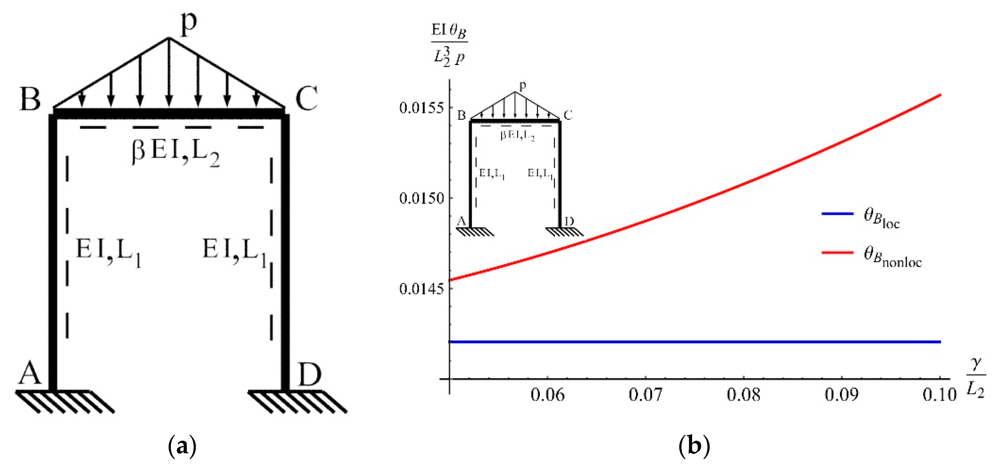
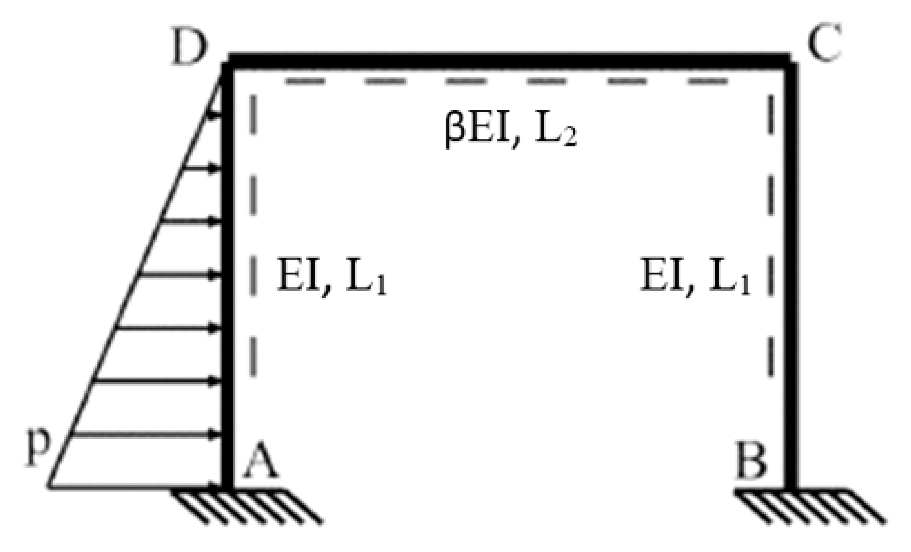
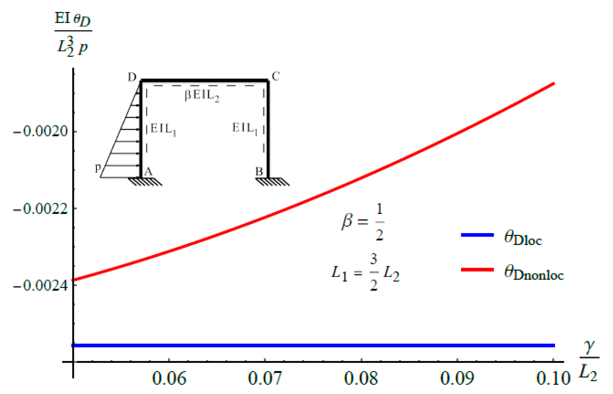
6.1. A Frame Subjected to Triangular Load

In this example, the moments at each joint of the frame shown in Figure 12a are obtained in the frame of nonlocal elasticity.

Equilibrium equations can be written in nodes B and C as follows [64] (see Equations (43) and (63)).

$$\left(\frac{4\beta EI}{L_2}\right.+\left.\frac{4EI}{L_1}\right) {\theta }_B+\frac{2\beta EI}{L_2} {\theta }_C+\frac{1}{96}p (48{\gamma }^2+5L_2{}^2)=0$$

(84)

$$\frac{2\beta EI}{L_2} {\theta }_B+\left(\frac{4\beta EI}{L_2}\right.+\left.\frac{4EI}{L_1}\right) {\theta }_C-\frac{1}{96}p (48{\gamma }^2+5L_2{}^2)=0$$

(85)

Solving Equations (84) and (85) simultaneously, ${\theta }_B$ and ${\theta }_C$ are found as follows.

$${\theta }_B=-\frac{L_1 L_{2}p (48{\gamma }^2+5L_2{}^2)}{192EI (\beta L_1+2L_2)}, {\theta }_C=\frac{p (48{\gamma }^2{L}_1 L_2+5L_1{L}_2{}^3)}{192EI (\beta L_1+2L_2)}$$

(86)

In the limit $\gamma$ goes to zero, ${\theta }_B$ and ${\theta }_C$ are

$$\underset{\gamma \to 0}{\lim } {\theta }_B=-\frac{5L_1 L_2{}^{3}p }{192\beta EI{L}_1+384EI{L}_2}, \underset{\gamma \to 0}{\lim } {\theta }_C=\frac{5L_1 L_2{}^{3}p }{192\beta EI{L}_1+384EI{L}_2}$$

(87)

The unit displacements obtained as a result of the present work are validated by the results given in [64] for $L_1$ = 12 m, $L_2$ = 8 m, $\beta$ = 1, $\gamma$ = 0, and p = 24 kN/m, for ${\theta }_B$ and ${\theta }_C$ (see

Table 1. Unit displacements for a frame system subjected to vertical triangular load [64].

Unit Displacements	$\mathbf{Reference} \mathbf{Study} (\mathit{\gamma }/\mathit{L}=0)$ [64]	$\mathbf{Present} (\mathit{\gamma }/\mathit{L}=0)$
${\theta }_B$	$-\frac{960}{7EI}$	$-\frac{960}{7EI}$
${\theta }_C$	$\frac{960}{7EI}$	$\frac{960}{7EI}$

).

$${\theta }_B=-\frac{960}{7EI}, {\theta }_C=\frac{960}{7EI}$$

(88)

Special Case: Variable cross section.

In the frame shown in Figure 12a, the variation of the moment of inertia and modulus of elasticity function of the elements AB and DC are (see Figure 13)

$$I(z)=-0.2 \frac{I}{L_1} z+1.2 I , E(z)=E+\frac{E}{L_1} z$$

(89)

For $L_1=12$ m, $m_{i {\theta }_i}$ is calculated using Equation (62) as follows.

$$m_{i {\theta }_i}=0.6015 EI$$

(90)

Equations (84) and (85) take the following form:

$$\begin{array}{l}\left.\left(\frac{4\beta EI}{L_2}\right.+0.6015EI\right) {\theta }_B+\frac{2\beta EI}{L_2} {\theta }_C+\frac{1}{96}p (48{\gamma }^2+5L_2{}^2)=0\\ \frac{2\beta EI}{L_2} {\theta }_B+\left.\left(\frac{4\beta EI}{L_2}\right.+0.6015EI\right){\theta }_C-\frac{1}{96}p (48{\gamma }^2+5L_2{}^2)=0\end{array}$$

(91)

${\theta }_B$ and ${\theta }_C$ are obtained by solving the system given in Equation (91).

$${\theta }_B=\frac{L_{2}p (-8.29182\beta {\gamma }^2-0.863731\beta L_2{}^2-0.831255{\gamma }^2{L}_2-0.0865891L_2{}^3)}{EI (33.1673{\beta }^2+13.3001\beta L_2+L_2{}^2)}=-{\theta }_C$$

(92)

For $L_1$ = 12 m, $L_2$ = 8 m, $\beta$ = 1, $\gamma$ = 0, and p = 24 kN/m,

$${\theta }_B=-\frac{93.9518}{EI}=-{\theta }_C$$

(93)

6.2. A Frame Subjected to Horizontal Triangular Load

In this section, a frame system subjected to non-symmetrical load is given as shown in Figure 14. Equilibrium equations can be written in nodes D and C and as follows [64] (see Equations (34), (35), (63) and (77)).

$$\begin{array}{l}\left(\frac{4EI}{L_1}+\frac{4\beta EI}{L_2}\right) {\theta }_D+\frac{2\beta EI}{L_2} {\theta }_C+\frac{2\beta EI{\theta }_C}{L_2}+\frac{6EI\delta }{L_1^2}-\frac{P{L}_1^2}{30}=0\\ \left(\frac{4EI}{L_1}+\frac{4\beta EI}{L_2}\right) {\theta }_C+\frac{2\beta EI{\theta }_D}{L_2}+\frac{6EI\delta }{L_1^2}=0\end{array}$$

(94)

The equilibrium condition in the AB direction is

$$\left(\frac{12EI}{L_1^3}+\frac{12EI}{L_1^3}\right)\delta +\frac{\left(\frac{4EI}{L_1}+\frac{2EI}{L_1}\right){\theta }_C}{L_1}+\frac{\left(\frac{4EI}{L_1}+\frac{2EI}{L_1}\right){\theta }_D}{L_1}-\frac{p{L}_1}{2}+\frac{7p{L}_1}{20}+\frac{{\gamma }^{2}p}{L_1}=0$$

(95)

${\theta }_C$, ${\theta }_D$, and $\delta$ are found by solving Equations (94) and (95) as follows.

$$\begin{array}{l}{\theta }_C=\frac{p{L}_1{L}_2\left(60\beta {\gamma }^2{L}_1-17\beta L_1^3+120{\gamma }^2{L}_2-12L_1^2{L}_2\right)}{240EI\left(6\beta L_1+L_2\right)\left(\beta L_1+2L_2\right)}\\ {\theta }_D=\frac{p{L}_1{L}_2\left(60\beta {\gamma }^2{L}_1+7\beta L_1^3+120{\gamma }^2{L}_2-8L_1^2{L}_2\right)}{240EI\left(6\beta L_1+L_2\right)\left(\beta L_1+2L_2\right)}\\ \delta =\frac{p{L}_1^2\left(-60\beta {\gamma }^2{L}_1+9\beta L_1^3-40{\gamma }^2{L}_2+4L_1^2{L}_2\right)}{240EI\left(6\beta L_1+L_2\right)}\end{array}$$

(96)

The unit displacements obtained as a result of the present work are validated by the results given in [64] for $L_1$ = 3 m, $L_2$ = 3 m, $\beta$ = 1, $\gamma$ = 0, and p = 30 kN/m, for ${\theta }_C$, ${\theta }_D$, and $\delta$ (see

Table 2. Unit displacements for a frame system subjected to horizontal triangular load [64].

Unit Displacements	$\mathbf{Reference} \mathbf{Study} (\mathit{\gamma }/\mathit{L}=0)$ [64]	$\mathbf{Present} (\mathit{\gamma }/\mathit{L}=0)$
${\theta }_C$	$-\frac{4.66}{EI}$	$-\frac{4.66}{EI}$
${\theta }_D$	$-\frac{0.161}{EI}$	$-\frac{0.161}{EI}$
$\delta$	$\frac{18.8}{EI}$	$\frac{18.8}{EI}$

).

The end moments can be written as below.

$$M_{AD}=-\left(\frac{2EI}{L_1}{\theta }_D+\frac{6EI}{L_1^2}\delta +\frac{1}{20}p\left(20{\gamma }^2+L_1^2\right)\right)$$

(97)

$$M_{DA}=\frac{4EI}{L}{\theta }_D+\frac{6EI}{L_1^2}\delta -\frac{p{L}_1^2}{30}$$

(98)

$$M_{DC}=-\left(\frac{2EI}{L_2}{\theta }_C+\frac{4EI}{L_2}{\theta }_D\right)$$

(99)

$$M_{CD}=\frac{2EI}{L_2}{\theta }_D+\frac{4EI}{L_2}{\theta }_C$$

(100)

$$M_{BC}=\frac{2EI}{L_1}{\theta }_C+\frac{6EI}{L_1^2}\delta$$

(101)

$$M_{CB}=-\left(\frac{4EI}{L_1}{\theta }_C+\frac{6EI}{L_1^2}\delta \right)$$

(102)

In the limit $\gamma$ goes to zero, the end moments (see

Table 3. End moments for a frame system subjected to horizontal triangular load [64].

End Moments	$\mathbf{Reference} \mathbf{Study} (\mathit{\gamma }/\mathit{L}=0)$ (kN.m) [64]	$\mathbf{Present} (\mathit{\gamma }/\mathit{L}=0)$ (kN.m)
$M_{AD}$	$-25.9$	$-25.9$
$M_{DA}$	$3.32$	$3.32$
$M_{DC}$	$3.32$	$3.32$
$M_{CD}$	$-6.32$	$-6.32$
$M_{BC}$	$9.43$	$9.48$
$M_{CB}$	$-6.32$	$-6.37$

) revert to the moments given in [64].

The variation of the rotation at the joint D in classical and nonlocal theory with respect to the $\gamma /L$ ratio is given in Figure 15.

7. Conclusions

In this paper, the slope deflection method for AFG beams with a variable cross section was presented in the frame of nonlocal elasticity. First, the transfer matrix was presented for AFG beams with a variable cross section. The stiffness coefficients and fixed-end moments were calculated systematically using MIV. Fixed-end moments of a beam subjected to distributed loads include the nonlocal parameter ($\gamma$) (see Section 4). It was observed that the nonlocal parameter was not included in the stiffness coefficients. That is, stiffness coefficients are independent of the nonlocality parameter (see Section 5). The difference between the moment values obtained by local and nonlocal theories grows significantly when the $\gamma /L$ ratio increases (see Figure 5a,b and Figure 8a,b). A similar situation also occurred in the rotation of joints in the frames (see Figure 12b). Therefore, the fixed-end moments calculated by nonlocal elasticity should be used in the static analysis of the nanostructures. All of the obtained results were validated by comparison to the reference study.

With the help of the present work, the unit displacement constants of the axially graded beams in different loading conditions were calculated using the given formulas. The obtained results were validated by comparison to the reference study. As statically indeterminate systems may contain many unknowns, solving such systems statically increases the computational load. This study offers an innovative approach in terms of easier analysis of systems such as frames of different dimensions that we encounter in engineering structures. The fact that the $\gamma /L$ ratio is zero in the study indicates the abandonment of the nanoscale and the transition to the classical state. Another important aspect of this study is that the relevant solutions are in a general form. That is, the solutions do not depend on the dimensions of the problem.

The authors agree that this study will be an important resource for structural engineering problems, wind turbine design, relatively small-sized electronic devices such as NEMS and MEMS, and the design of biomedical devices. We also believe that a more advanced composite material model can be obtained by designing the beam as a bi-directional structure, in addition to the structure of axially graded beams in the current study.

References

1. Chen, J. Nonlocal Euler-Bernoulli Beam Theories, 1st ed.; Springer: Cham, Switzerland, 2021; pp. 1–7. [Google Scholar]
2. Çelik, M. Mechanical Behavior of the Bi-Directional Beams. Ph.D. Thesis, Istanbul Technical University, Istanbul, Turkey, 2021. [Google Scholar]
3. Demirkan, E. Investigation of Buckling Analysis Based on Nonlocal Timoshenko Rods by the Method of Initial Values. Ph.D. Thesis, Istanbul Technical University, Istanbul, Turkey, 2020. [Google Scholar]
4. Demirkan, E.; Artan, R. Buckling analysis of nanobeams based on nonlocal Timoshenko beam model by the method of initial values. Int. J. Struct. Stab. Dyn. 2018, 19, 1950036. [Google Scholar] [CrossRef]
5. Nejad, M.; Hadi, A.; Omidvari, A.; Rastgoo, A. Bending analysis of bi-directional functionally graded Euler-Bernoulli nano-beamsusing integral form of Eringen’s nonlocal elasticity theory. Struct. Eng. Mech. 2018, 67, 417–425. [Google Scholar]
6. Husain, M.A.; Hasan, Z.H. Reduced Equations of Slope-Deflection Method in Structural Analysis. Int. J. Appl. Mech. Eng. 2021, 26, 51–62. [Google Scholar] [CrossRef]
7. Kassimali, A. Structural Analysis, 8th ed.; Cengage Learning Inc.: Boston, MA, USA, 2020; pp. 20–42. [Google Scholar]
8. Mau, S.T. Introduction to Structural Displacement and Force Methods, 1st ed.; Taylor and Francis Group: Boca Raton, FL, USA, 2012; pp. 197–218. [Google Scholar]
9. McCormac, J.C. Structural Analysis Using Classical and Matrix Methods, 4th ed.; John Wiley and Sons Inc.: Hoboken, NJ, USA, 2012; pp. 363–388. [Google Scholar]
10. Yoshida, S. Analysis of rigid frames in space by applying slope-deflection formulas. J. Fac. Eng. 1961, 12, 35–112. [Google Scholar]
11. Backer, H.D.; Outtier, A.; Bogaert, P.V. Analytical calculation of internal forces in orthotropic plated bridge decks based on the slope-deflection method. J. Constr. Steel Res. 2008, 64, 1530–1539. [Google Scholar] [CrossRef]
12. Aristizabal-Ochoa, J.D. Stability and Second-Order Analysis of Timoshenko Beam-Column Structures with Semi-Rigid Connections: Slope-Deflection Method. DYNA 2009, 76, 7–21. [Google Scholar] [CrossRef]
13. Arshid, E.; Amir, S. Size-dependent vibration analysis of fluid-infiltrated porous curved microbeams integrated with reinforced functionally graded graphene platelets face sheets considering thickness stretching effect. Proc. Inst. Mech. Eng. Part L J. Mater. Des. Appl. 2021, 235, 1077–1099. [Google Scholar] [CrossRef]
14. Mudhaffar, I.M.; Tounsi, A.; Chikh, A.; Al-Osta, M.A.; Al-Zahrani, M.M.; Al-Dulaijan, S.U. Hygro-thermo-mechanical bending behavior of advanced functionally graded ceramic metal plate resting on a viscoelastic foundation. Structures 2021, 33, 2177–2189. [Google Scholar] [CrossRef]
15. Belarbi, M.O.; Garg, A.; Houari, M.S.A.; Hirane, H.; Tounsi, A.; Chalak, H.D. A three-unknown refined shear beam element model for buckling analysis of functionally graded curved sandwich beams. Eng. Comput. 2021, 38, 4273–4300. [Google Scholar] [CrossRef]
16. Babaei, M.; Kiarasi, F.; Tehrani, M.S.; Hamzei, A.; Mohtarami, E.; Asemi, K. Three dimensional free vibration analysis offunctionally graded graphene reinforced composite laminated cylindrical panel. Proc. Inst. Mech. Eng. Part L J. Mater. Des. Appl. 2022, 236, 1501–1514. [Google Scholar]
17. Chen, Y.; Dong, S.; Zang, Z.; Gao, M.; Zhang, J.; Ao, C.; Liu, H.; Zhang, Q. Free transverse vibrational analysis of axiallyfunctionally graded tapered beams via the variational iteration approach. J. Vib. Control 2021, 27, 1265–1280. [Google Scholar] [CrossRef]
18. Karamanli, A.; Aydogdu, M. Buckling of laminated composite and sandwich beams due to axially varying in-plane loads. Compos. Struct. 2019, 210, 391–408. [Google Scholar] [CrossRef]
19. Patil, H.H.; Pitchaimani, J.; Eltaher, M.A. Buckling and vibration of beams using Ritz method: Effects of axial grading of GPL and axially varying load. Mech. Adv. Mater. Struct. 2023, 30, 1–14. [Google Scholar] [CrossRef]
20. Shafiei, N.; Hamisi, M.; Ghadiri, M. Vibration analysis of rotary tapered axially functionally graded Timoshenko nanobeam in thermal environment. J. Solid Mech. 2020, 12, 16–32. [Google Scholar]
21. Akbaş, Ş.D. Geometrically nonlinear analysis of axially functionally graded beams by using finite element method. J. Comput. Appl. Mech. 2020, 51, 411–416. [Google Scholar]
22. Wang, Y.; Ren, H.; Fu, T.; Shi, C. Hygrothermal mechanical behaviors of axially functionally graded microbeams using a refined first order shear deformation theory. Acta Astronaut 2020, 166, 306–316. [Google Scholar] [CrossRef]
23. Khaniki, H.B.; Ghayesh, M.H. On the dynamics of axially functionally graded CNT strengthened deformable beams. Eur. Phys. J. Plus 2020, 135, 415. [Google Scholar] [CrossRef]
24. Yee, K.; Kankanamalage, U.M.; Ghayesh, M.H.; Jiao, Y.; Hussain, S.; Amabili, M. Coupled dynamics of axially functionally graded graphene nanoplatelets-reinforced viscoelastic shear deformable beams with material and geometric imperfections. Eng. Anal. Bound. Elem. 2022, 136, 4–36. [Google Scholar] [CrossRef]
25. Gantayat, A.K.; Sutar, M.K.; Mohanty, J.R. Dynamic characteristic of graphene reinforced axial functionally graded beam using finite element analysis. Mater. Today Proc. 2022, 62, 5923–5927. [Google Scholar] [CrossRef]
26. Hamed, M.A.; Mohamed, S.A.; Eltaher, M.A. Buckling analysis of sandwich beam rested on elastic foundation and subjected to varying axial in-plane loads. Steel Compos. Struct. Int. J. 2020, 34, 75–89. [Google Scholar]
27. Alazwari, M.A.; Mohamed, S.A.; Eltaher, M.A. Vibration analysis of laminated composite higher order beams under varying axial loads. Ocean Eng. 2022, 252, 111203. [Google Scholar] [CrossRef]
28. Harsha, B.P.; Jeyaraj, P.; Lenin, B.M.C. Effect of porosity and profile axial loading on elastic buckling and free vibration of functionally graded porous beam. In Proceedings of the IOP Conference Series: Materials Science and Engineering, Chennai, India, 31 October 2020. [Google Scholar]
29. Priyanka, R.; Twinkle, C.M.; Pitchaimani, J. Stability and dynamic behavior of porous FGM beam: Influence of graded porosity, graphene platelets, and axially varying loads. Eng. Comput. 2022, 38, 4347–4366. [Google Scholar] [CrossRef]
30. Huang, Y.; Li, X.F. A new approach for free vibration of axially functionally graded beams with non-uniform cross-section. J. Sound Vib. 2010, 329, 2291–2303. [Google Scholar] [CrossRef]
31. Anandakumar, G.; Kim, J.H. On the modal behavior of a three-dimensional functionally graded cantilever beam: Poisson’s ratio and material sampling effects. Compos. Struct. 2010, 92, 1358–1371. [Google Scholar] [CrossRef]
32. Ait Atmane, H.; Tounsi, A.; Meftah, S.A.; Belhadj, H.A. Free vibration behavior of exponential functionally graded beams with varying cross-section. J. Vib. Control 2011, 17, 311–318. [Google Scholar] [CrossRef]
33. Li, X.F.; Kang, Y.A.; Wu, J.X. Exact frequency equations of free vibration of exponentially functionally graded beams. Appl. Acoust. 2013, 74, 413–420. [Google Scholar] [CrossRef]
34. Koizumi, M. Use of Composites Multi-Phased and Functionally Graded Materials. Compos. Part B Eng. 1997, 28, 1–4. [Google Scholar] [CrossRef]
35. Birman, V.; Byrd, L.W. Modeling and analysis of functionally graded materials and structures. ASME Appl. Mech. Rev. 2007, 60, 195–216. [Google Scholar] [CrossRef]
36. Sankar, B.V. An elasticity solution for functionally graded beams. Compos. Sci. Technol. 2001, 61, 689–696. [Google Scholar] [CrossRef]
37. Bhangale, R.K.; Ganesan, N. Thermoelastic buckling and vibration behavior of a functionally graded sandwich beam with constrained viscoelastic core. J. Soundand Vib. 2006, 295, 294–316. [Google Scholar] [CrossRef]
38. Chakraborty, A.; Gopalakrishnan, S.; Reddy, J.N. A new beam finite element for the analysis of functionally graded materials. Int. J. Mech. Sci. 2003, 45, 519–539. [Google Scholar] [CrossRef]
39. Chakraborty, A.; Gopalakrishnan, S. A spectrally formulated finite element for wave propagation analysis in functionally graded beams. Int. J. Solids Struct. 2003, 40, 2421–2448. [Google Scholar] [CrossRef]
40. Kadoli, R.; Akhtar, K.; Ganesan, N. Static analysis of functionally graded beams using higher order shear deformation theory. Appl. Math. Model. 2008, 32, 2509–2525. [Google Scholar] [CrossRef]
41. Li, K.V.S.G. Buckling of functionally graded and elastically restrained non-uniform columns. Compos. Part B Eng. 2009, 40, 393–403. [Google Scholar]
42. Alshorbagy, A.E.; Eltaher, M.A.; Mahmoud, F.F. Free vibration characteristics of a functionally graded beam by finite element method. Appl. Math. Model. 2011, 35, 412–425. [Google Scholar] [CrossRef]
43. Banerjee, J.R.; Ananthapuvirajah, A. Free vibration of functionally graded beams and frameworks using the dynamic stiffness method. J. Sound Vib. 2018, 422, 34–47. [Google Scholar] [CrossRef]
44. Zhang, K.; Ge, M.H.; Zhao, C.; Deng, Z.C.; Xu, X.J. Free vibration of nonlocal Timoshenko beams made of functionally graded materials by symplectic method. Compos. Part B Eng. 2019, 156, 174–184. [Google Scholar] [CrossRef]
45. Cao, D.; Gao, Y. Free vibration of non-uniform axially functionally graded beams using the asymptotic development method. Appl. Math. Mech. 2019, 40, 85–96. [Google Scholar] [CrossRef]
46. Elishakoff, I.; Candan, S. Apparently first closed-form solution for vibrating: Inhomogeneous beams. Int. J. Solids Struct. 2001, 38, 3411–3441. [Google Scholar] [CrossRef]
47. Çelik, M.; Artan, R. An investigation of static bending of a bi-directional strain-gradient Euler–Bernoulli nano-beams with the method of initial values. Microsyst. Technol. 2020, 26, 2921–2929. [Google Scholar] [CrossRef]
48. Çelik, M.; Artan, R. Buckling Analysis of a Bi-Directional Strain-Gradient Euler–Bernoulli Nano-Beams. Int. J. Struct. Stab. Dyn. 2020, 20, 2050114. [Google Scholar] [CrossRef]
49. Calim, F.F. Transient analysis of axially functionally graded Timoshenko beams with variable cross-section. Compos. Part B Eng. 2016, 98, 472–483. [Google Scholar] [CrossRef]
50. Shahba, A.; Attarnejad, R.; Marvi, M.T.; Hajilar, S. Free vibration and stability analysis of axially functionally graded tapered Timoshenko beams with classical and non-classical boundary conditions. Compos. Part B Eng. 2011, 42, 801–808. [Google Scholar] [CrossRef]
51. Huang, Y.; Yang, L.E.; Luo, Q.Z. Free vibration of axially functionally graded Timoshenko beams with non-uniform cross-section. Compos. Part B Eng. 2013, 45, 1493–1498. [Google Scholar] [CrossRef]
52. Zhao, Y.; Huang, Y.; Guo, M. A novel approach for free vibration of axially functionally graded beams with non-uniform cross section based on Chebyshev polynomials theory. Compos. Struct. 2017, 168, 277–284. [Google Scholar] [CrossRef]
53. Bambill, D.V.; Rossit, C.A.; Felix, D.H. Free vibrations of stepped axially functionally graded Timoshenko beams. Meccanica 2015, 50, 1073–1087. [Google Scholar] [CrossRef]
54. Shvartsman, B.; Majak, J. Numerical method for stability analysis of functionally graded beams on elastic foundation. Appl. Math. Model. 2016, 40, 3713–3719. [Google Scholar] [CrossRef]
55. Chen, X.W.; Yue, Z.Q. Contact mechanics of two elastic spheres reinforced by functionally graded materials (FGM) thin coaitngs. Eng. Anal. Bound. Elem. 2019, 109, 57–69. [Google Scholar] [CrossRef]
56. Li, L.; Hu, Y. Wave propagation in fluid-conveying viscoelastic carbon nanotubes based on nonlocal strain gradient theory. Comput. Mater. Sci. 2016, 112, 282–288. [Google Scholar] [CrossRef]
57. Li, L.; Hu, Y.; Ling, L. Wave propagation in viscoelastic single-walled carbon nanotubes with surface effect under magnetic field based on nonlocal strain gradient theory. Phys. E Low-Dimens. Syst. Nanostruct. 2016, 75, 118–124. [Google Scholar] [CrossRef]
58. Narendar, S.; Gopalakrishnan, S. Nonlocal scale effects on wave propagation in multi-walled carbon nanotubes. Comput. Mater. Sci. 2009, 47, 526–538. [Google Scholar] [CrossRef]
59. Nazemnezhad, R.; Hosseini-Hashemi, S. Nonlocal nonlinear free vibration of functionally graded nanobeams. Compos. Struct. 2014, 110, 192–199. [Google Scholar] [CrossRef]
60. Rahmani, O.; Jandaghian, A.A. Buckling analysis of functionally graded nanobeams based on a nonlocal third-order shear deformation theory. Appl. Phys. A 2015, 119, 1019–1032. [Google Scholar] [CrossRef]
61. Liang, Y.; Han, Q. Prediction of the nonlocal scaling parameter for graphene sheet. Eur. J. Mech. A/Solids 2014, 45, 153–160. [Google Scholar] [CrossRef]
62. Peddieson, J.; Buchanan, G.R.; McNitt, R.P. Application of nonlocal continuum models to nanotechnology. Int. J. Eng. Sci. 2003, 41, 305–312. [Google Scholar] [CrossRef]
63. Artan, R.; Toksöz, A. Stability analysis of gradient elastic beams by the method of initial value. Arch. Appl. Mech. 2013, 83, 1129–1144. [Google Scholar] [CrossRef]
64. Hibbeler, A. Structural Analysis, 8th ed.; Pearson Prentice Hall, Pearson Education, Inc.: Upper Saddle River, NJ, USA, 2012; Volume 07458, pp. 470–484. [Google Scholar]
65. Chen, W.R.; Chang, H. Closed-form solutions for free vibration frequencies of functionally graded Euler-Bernoulli beams. Mech. Compos. Mater. 2017, 53, 79–98. [Google Scholar] [CrossRef]
66. Kahya, V.; Turan, M. Finite element model for vibration and buckling of functionally graded beams based on the first-order shear deformation theory. Compos. Part B Eng. 2017, 109, 108–115. [Google Scholar] [CrossRef]
67. Khiem, N.T.; Tran, H.T.; Nam, D. Modal analysis of cracked continuous Timoshenko beam made of functionally graded material. Mech. Based Des. Struct. Mach. 2019, 48, 459–479. [Google Scholar] [CrossRef]
68. Eringen, A.C. On differential equations of nonlocal elasticity and solutions of screw dislocation and surface waves. J. Appl. Phys. 1983, 54, 4703–4710. [Google Scholar] [CrossRef]
Figure 1. (a) A beam subjected to a distributed load; (b) a beam subjected to two different loads.
Applsci 13 04814 g001
Figure 2. (a) Beam subjected to singular force; (b) both ends of a fixed beam subjected to a distributed load.
Applsci 13 04814 g002
Figure 3. (a) Positive directions in MIV; (b) positive directions in SDM.
Applsci 13 04814 g003
Figure 4. (a) Beam subjected to the uniform load; (b) beam subjected to the triangular load.
Applsci 13 04814 g004
Figure 5. (a) The variation of the initial moment ( M 0 ); (b) the variation of the end moment ( M L ).
Applsci 13 04814 g005
Figure 6. A fixed beam with both ends subjected to the two different distributed loads.
Applsci 13 04814 g006
Figure 7. (a) Uniform beam with a constant cross section subjected to the two different uniform loads; (b) uniform beam with a constant cross section subjected to the two different triangular loads.
Applsci 13 04814 g007
Figure 8. (a) The variation of the initial moment ( M 0 ); (b) the variation of the initial moment ( M 0 ).
Applsci 13 04814 g008
Figure 9. (a) Fixed beam with both ends subjected to singular force; (b) fixed-pinned beams subjected to singular force.
Applsci 13 04814 g009
Figure 12. (a) The frame subjected to the two triangular loads ( p ) ; (b) the variation of rotation ( θ B ) at point B.
Applsci 13 04814 g012
Figure 13. The variation of the moment of inertia of the elements AB and DC (see Figure 12a).
Applsci 13 04814 g013
Figure 14. Frame subjected to non-symmetrical loading ( p ) .
Applsci 13 04814 g014
Figure 15. The variation of the rotation at the joint D.
Applsci 13 04814 g015