Extended Smoothing Methods for Sparse Test Data Based on Zero-Padding

Abstract

Aiming at the problem of sparse measurement points due to test conditions in engineering, a smoothing method based on zero-padding in the wavenumber domain is proposed to increase data density. Firstly, the principle of data extension and smoothing is introduced. The core idea of this principle is to extend the discrete data series by zero-padding in the wavenumber domain. The conversion between the spatial and wavenumber domains is achieved using the Discrete Fourier Transform (DFT) and the Inverse Discrete Fourier Transform (IDFT). Then, two sets of two-dimensional discrete random data are extended and smoothed, respectively, and the results verify the effectiveness and feasibility of the algorithm. The method can effectively increase the density of test data in engineering tests, achieve smoothing and extend the application to areas related to data processing.

1. Introduction

In engineering practice, affected by the test conditions, often only sparse test data can be obtained. For example, the geographical environment test cannot fully test the environmental information of each point, and it is necessary to smooth the test data based on a limited number of observations to get the overall terrain data [1]. These problems also arise in the fields of sound [2] and image processing [3]. As a result, obtaining more complete results based on sparse test data has become a key research priority. Smoothing sparse test data can not only solve the problem of too little test data but also, to a certain extent, speed up the processes of data acquisition, processing, and practical application.

Interpolation methods have been proposed to smooth sparse test data for the purpose of enhancing the characteristics of the data under study [4,5]. The main interpolation methods include Lagrange fitting [6,7], piecewise cubic Hermite fitting [8,9,10,11], least squares [2,3,12], cubic spline curve method [13,14] and others. To expand on this, Wang first established the least squares regression model using the measurement data of the two-dimensional laser sensor in order to accurately extract the wheel contour, and then applied the Lagrange multiplication to obtain the least squares solution of the parameters, which gave a smooth and continuous contour [6]. Data from second-order systems can be more easily fitted using the algebraic hyperbolic cubic Hermite spline interpolation approach provided by Oraiche et al. [8]. The above two interpolation methods have a narrow application range, and there are some problems such as non-convergence and non-smoothness of piecewise linear interpolation function at nodes, while the cubic spline function can solve the above problems and the calculation is simple. The cubic spline function can pass through all sampling points and has a second continuous derivative, which is an ideal interpolation tool [15]. Wu et al. improved the cubic spline interpolation method, solved the problem of cubic spline interpolation of dynamic curves, and enabled the measured discrete signals to form a smooth curve [16]. Liu et al. studied the advantages and disadvantages of ordinary Kriging interpolation, cubic spline interpolation and inverse distance weight reciprocal interpolation, aiming to guide researchers to choose appropriate spatial interpolation methods according to their actual measurement needs [17]. Each of these curve smoothing methods has its own advantages, but they also have some limitations. The advantage is that they greatly improve the smoothness and accuracy of the curve; the limitation is that they can only be used under specific conditions and are not universal.

In addition, zero-padding of the angular spectrum allows for an increase in data resolution [18,19,20]. Some scholars discussed the zero-padding problem of one-dimensional Fourier transform, and obtained the spectrum value by the zero-padding of one-dimensional test data. In contrast, this paper focuses on the zero-padding of the wavenumber domain data (i.e., the angular spectrum) after the two-dimensional Fourier transform. Furthermore, a number of other scholars are also working on such data processing issues [21]. They optimize the traditional FFT/IFFT method to get better imaging performance when studying 3D imaging. Kim performs a phase shift to compensate the spherical wave effect after an FFT, and the efficiency and accuracy are comparable in the case of full sampling [22]. Kan applies zero-padding to interpolate the spectrum of the sampled signal and finally obtains the three-dimensional human image [23]. In addition, in the field of frequency estimation, Xiang et al. can estimate the frequency of complex sinusoidal signals flexibly and accurately by using DFT interpolation and zero-padding on the original input data [24].

The basic core concept of this study, which is based on the DFT operation and zero-padding, is an extended smoothing method for two-dimensional discrete data. The DFT operation has the characteristics of fast computation and transformation between the spatial domain and the wavenumber domain. The zero-padding and partial angular spectral adjustment operation has the characteristics of data expansion. Combining the properties of these two methods allows for extended smoothing of discrete data in two dimensions.

The smoothing method proposed in this paper is mainly suitable for sparse sampling data measured in engineering tests. It is possible to improve the density of sampling data to obtain a smoother distribution of measured spatial data.

2. The Smoothing Theory of Two-Dimensional Discrete Data

The core idea of two-dimensional discrete data smoothing theory is to extend the discrete data series by zero-padding in the wavenumber domain. The transformation between the spatial domain and the wavenumber domain is mainly realized by the two-dimensional Fourier transform method, and its process block diagram is shown in Figure 1.

The smoothing process for two-dimensional discrete data is shown in Figure 1, and the process consists of three main steps.

In the first step, the discrete signal is transformed from the spatial domain to the wavenumber domain by two-dimensional DFT. It is complicated to process discrete data in the spatial domain, but the data can be transformed into the wavenumber domain by DFT to process its angular spectrum.

In the second step, the above angular spectrum sequence is supplemented with zeros to artificially expand its sequence, and the angular spectrum value at a specific position is changed accordingly. This procedure complements the original sequence with zeroes but does not add any additional information to the angular spectrum in the wavenumber domain.

In the third step, the newly generated angular spectrum in the wavenumber domain is transformed into the spatial domain by two-dimensional IDFT, and a new two-dimensional discrete signal is obtained. Smoothing produces the discrete signal that was regenerated.

3. Calculation Process of Smoothing Theory

3.1. DFT

Firstly, the discrete signal is transformed from the spatial domain to the wavenumber domain by two-dimensional DFT. The reason for this is that it is more complicated to deal with discrete data in the spatial domain and simpler in the wavenumber domain. The specific steps are as follows.

Equation (1) is a two-dimensional continuous Fourier transform formula which transforms the two-dimensional spatial signal p (x, y) to the wavenumber domain to obtain the angular spectrum P (k_x, k_y).

$$P\left(k_x,k_y\right)={\displaystyle \underset{0}{\overset{L_x}{\int }}{\displaystyle \underset{0}{\overset{L_y}{\int }}p\left(x,y\right)H\left(x,y\right)e^{-i\left(k_{x}x+k_{y}y\right)}dxdy}}$$

(1)

in which H (x, y) is the spatial window function. L_x and L_y are the length and width of the test space, respectively.

For a finite test space, the edges are discontinuous. In order to reduce the error caused by discontinuity, a spatial window function H (x, y) is introduced. The 8-point Tukey window function can be written as follows:

$$H\left(x,y\right)=\left\{\begin{array}{cc}1& x\le \frac{L_x}{2}-w_{x}andy\le \frac{L_y}{2}-w_y\\ \begin{array}{l}\left[\frac{1}{2}-\frac{1}{2}\cos \left(\frac{\pi \left(x-L_x/2\right)}{w_x}\right)\right]\\ \times \left[\frac{1}{2}-\frac{1}{2}\cos \left(\frac{\pi \left(y-L_y/2\right)}{w_y}\right)\right]\end{array}& \frac{L_x}{2}-w_x<x<\frac{L_x}{2}or\frac{L_y}{2}-w_y<y<\frac{L_y}{2}\\ 0& x\ge \frac{L_x}{2}ory\ge \frac{L_y}{2}\end{array}\right.$$

(2)

in which w_x = 8Δx is the width of the spatial window function along the x direction, and w_y = 8Δy is the width of the spatial window function along the y direction.

In engineering applications, the two-dimensional spatial continuous signal needs to be discretized, and then the discrete space is processed by DFT to transform the discrete data from the spatial domain to the wavenumber domain, which can provide the angular spectrum value,

$$P(n_x\Delta k_x,n_y\Delta k_y)=\Delta x\Delta y{\displaystyle \sum _{m_x=0}^{Nx-1}{\displaystyle \sum _{m_y=0}^{Ny-1}p(m_x\Delta x,m_y\Delta y)}}H\left(m_x\Delta x,m_y\Delta y\right)e^{-j2\pi \left(\frac{n_x{m}_x}{Nx}+\frac{n_y{m}_y}{Ny}\right)}$$

(3)

in which p (m_xΔx, m_yΔy) represents a two-dimensional spatial discrete signal. Δx and Δy are the sampling intervals along the x and y directions, respectively. m_x and m_y are the discrete spatial variables along the x and y directions, respectively. n_x and n_y are discrete variables along the k_x and k_y directions in the wavenumber domain, respectively. N_x and N_y represent the number of discrete points in the spatial domain (or wavenumber domain), respectively. Δk_x = 2π/N_x and Δk_y = 2π/N_y are wavenumber domain intervals, and k_x = n_xΔk_x and k_y = n_yΔk_y are variables. j is an imaginary unit.

3.2. Zero-Padding

The angular spectrum in the wavenumber domain is extended by zero-padding, and the angular spectrum value of a specific position is changed accordingly. This zero-padding operation does not add additional information about the wavenumber angular spectrum in the wavenumber domain. The specific steps are as follows.

The generated angular spectrum P’ is acquired by zero-padding of the original angular spectrum P. The data numbers of the original angular spectrum in k_x and k_y direction are N_x and N_y, respectively, and those of the generated angular spectrum are 2N_x and 2N_y, respectively.

When the original angular spectrum is zero-padded and extended, the generated angular spectrum value is twice the original angular spectrum value at the following positions:

$$\left\{\begin{array}{ll}{P}^{\prime }(n_x\Delta k_x,n_y\Delta k_y)=2P(n_x\Delta k_x,n_y\Delta k_y)\hfill & n_x=0,\cdots ,\frac{Nx}{2}-1;n_y=0,\cdots ,\frac{Ny}{2}-1\hfill \\ P^{\prime }\left(\left(n_x+Nx\right)\Delta k_x,n_y\Delta k_y\right)=2P(n_x\Delta k_x,n_y\Delta k_y)\hfill & n_x=\frac{Nx}{2}+1,\cdots ,Nx-1;n_y=0,\cdots ,\frac{Ny}{2}-1\hfill \\ P^{\prime }\left(n_x\Delta k_x,\left(n_y+Ny\right)\Delta k_y\right)=2P(n_x\Delta k_x,n_y\Delta k_y)\hfill & n_x=0,\cdots ,\frac{Nx}{2}-1;n_y=\frac{Ny}{2}+1,\cdots ,Ny-1\hfill \\ P^{\prime }\left(\left(n_x+Nx\right)\Delta k_x,\left(n_y+Ny\right)\Delta k_y\right)=2P(n_x\Delta k_x,n_y\Delta k_y)\hfill & n_x=\frac{Nx}{2}+1,\cdots ,Nx-1;n_y=\frac{Ny}{2}+1,\cdots ,Ny-1\hfill \end{array}\right.$$

(4)

At the following specified positions, the generated angular spectrum value remains the same as the original angular spectrum value, as shown in Equation (5):

$$\left\{\begin{array}{ll}{P}^{\prime }(\frac{Nx}{2}\Delta k_x,n_y\Delta k_y)=P(\frac{Nx}{2}\Delta k_x,n_y\Delta k_y)\hfill & n_y=0,\cdots ,\frac{Ny}{2}-1\hfill \\ P^{\prime }(\frac{3Nx}{2}\Delta k_x,n_y\Delta k_y)=P(\frac{Nx}{2}\Delta k_x,n_y\Delta k_y)\hfill & n_y=0,\cdots ,\frac{Ny}{2}-1\hfill \\ P^{\prime }(n_x\Delta k_x,\frac{Ny}{2}\Delta k_y)=P(n_x\Delta k_x,\frac{Ny}{2}\Delta k_y)\hfill & n_x=0,\cdots ,\frac{Nx}{2}-1\hfill \\ P^{\prime }(\left(n_x+Nx\right)\Delta k_x,\frac{Ny}{2}\Delta k_y)=P(n_x\Delta k_x,\frac{Ny}{2}\Delta k_y)\hfill & n_x=\frac{Nx}{2}+1,\cdots ,Nx-1\hfill \\ P^{\prime }(n_x\Delta k_x,\frac{3Ny}{2}\Delta k_y)=P(n_x\Delta k_x,\frac{Ny}{2}\Delta k_y)\hfill & n_x=0,\cdots ,\frac{Nx}{2}-1\hfill \\ P^{\prime }(\frac{Nx}{2}\Delta k_x,\left(n_y+Ny\right)\Delta k_y)=P(\frac{Nx}{2}\Delta k_x,n_y\Delta k_y)\hfill & n_y=\frac{Ny}{2}+1,\cdots ,Ny-1\hfill \\ P^{\prime }(\left(n_x+Nx\right)\Delta k_x,\frac{3Ny}{2}\Delta k_y)=P(n_x\Delta k_x,\frac{Ny}{2}\Delta k_y)\hfill & n_x=\frac{Nx}{2}-1,\cdots ,Nx-1\hfill \\ P^{\prime }(\frac{3Nx}{2}\Delta k_x,\left(n_y+Ny\right)\Delta k_y)=P(\frac{Nx}{2}\Delta k_x,n_y\Delta k_y)\hfill & n_y=\frac{Ny}{2}+1,\cdots ,Ny-1\hfill \end{array}\right.$$

(5)

At the following specified positions, the generated angular spectrum value is reduced to half of the original angular spectrum value, as shown in Equation (6):

$$\left\{\begin{array}{c}{P}^{\prime }(\frac{Nx}{2}\Delta k_x,\frac{Ny}{2}\Delta k_y)=\frac{1}{2}P(\frac{Nx}{2}\Delta k_x,\frac{Ny}{2}\Delta k_y)\\ P^{\prime }(\frac{3Nx}{2}\Delta k_x,\frac{Ny}{2}\Delta k_y)=\frac{1}{2}P(\frac{Nx}{2}\Delta k_x,\frac{Ny}{2}\Delta k_y)\\ P^{\prime }(\frac{Nx}{2}\Delta k_x,\frac{3Ny}{2}\Delta k_y)=\frac{1}{2}P(\frac{Nx}{2}\Delta k_x,\frac{Ny}{2}\Delta k_y)\\ P^{\prime }(\frac{3Nx}{2}\Delta k_x,\frac{3Ny}{2}\Delta k_y)=\frac{1}{2}P(\frac{Nx}{2}\Delta k_x,\frac{Ny}{2}\Delta k_y)\end{array}\right.$$

(6)

Except for the specific positions given above, the generated angular spectrum values are zero at all positions.

The data numbers of the generated angular spectrum in k_x and k_y directions are Nx’ = 2Nx and Ny’ = 2Ny, respectively. Thus m_x’ = 0, 1, 2,…, 2N_x − 1 and m_y’ = 0, 1, 2,…, 2N_y − 1. The ranges of n_x’ and n_y’ are the same as m_x’ and m_y’, respectively. The spatial sampling intervals are Δx’ = Δx/2 and Δy’ = Δy/2.

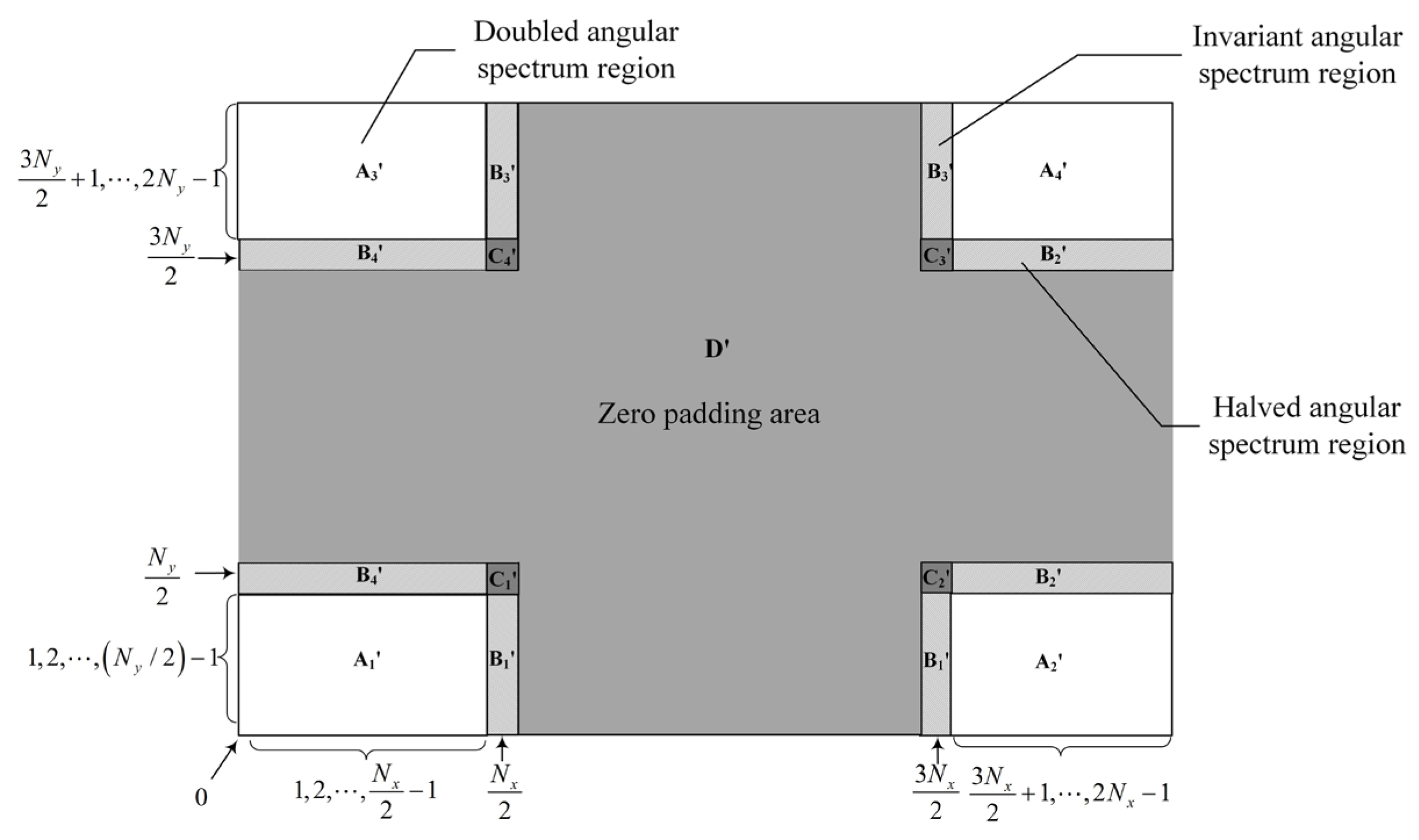
The following is a visual illustration of the zero-padded extension through a two-dimensional planar graph. Firstly, the coordinate value of the z axis is ignored, and only the angular spectrum distribution region of the x and y planes is studied. Then the distribution of the original angular spectrum is divided into three regions: A, B and C, as shown in Figure 2. Region A contains four small regions A₁, A₂, A₃ and A₄, and region B contains four small regions: B₁, B₂, B₃ and B₄.

Finally, the change of angular spectrum value in each region after zero-padded expansion is analyzed, and the division of each region is shown in Figure 3.

Figure 2 and Figure 3 clearly show the change of angular spectrum in the process of zero-padded expansion. Region A is the angular spectrum before smoothing. Region A′ is the angular spectrum after smoothing, and so on. The region of the original angular spectrum is divided into three regions: A, B, and C. The generated angular spectrum region after zero-padded expansion includes four regions, A′, B′, C′ and D′, among which the newly added region D′ is the zero-padded region. In addition, region A contains four small regions: A₁, A₂, A₃ and A₄. After zero-padded expansion, region A is separated into new positions, and the specific numerical coordinates are shown in Figure 3. Region B is split into two B′ regions due to the zero-padded expansion, and region C becomes four new C′ regions.

In terms of the value of angular spectrum, the value of region A′ is twice that of the corresponding region A. The value of region B′ is the same as that of corresponding region B; The value of region C′ is reduced to half of that of region C. Region D′ is the zero-padded region, and the angular spectrum values are all zeros.

3.3. IDFT

A new two-dimensional discrete signal is obtained after the newly generated domain angular spectrum in the wavenumber domain is translated to the spatial domain via two-dimensional IDFT. The regenerated discrete signal is the result of smoothing. The detailed steps are as follows.

The angular spectrum P (k_x, k_y) is performed by IDFT to obtain its spatial distribution:

$$p\left(x,y\right)=\frac{1}{4{\pi }^2}{\displaystyle \underset{-k_{\max ,x}}{\overset{+k_{\max ,x}}{\int }}{\displaystyle \underset{-k_{\max ,y}}{\overset{+k_{\max ,y}}{\int }}P\left(k_x,k_y\right)e^{i\left(k_{x}x+k_{y}y\right)}W\left(k_x,k_y\right)\mathrm{d}{k}_x\mathrm{d}{k}_y}}$$

(7)

in which W (k_x, k_y) depict the k-space filter.

According to Equation (7), the generated angular spectrum P’ (k_x, k_y) is transformed from the wavenumber domain to the spatial domain to obtain new discrete data p’ (x, y) by using the two-dimensional IDFT. This discrete signal p’ (x, y) is the smoothing result.

$$\begin{array}{l}{p}^{\prime }(m_x{}^{\prime }\Delta x^{\prime },m_y{}^{\prime }\Delta y^{\prime })=\frac{1}{2N{x}^{\prime }N{y}^{\prime }\Delta x^{\prime }\Delta y^{\prime }}\\ {\displaystyle \sum _{n_x{}^{\prime }=0}^{N{x}^{\prime }-1}{\displaystyle \sum _{n_y{}^{\prime }=0}^{N{y}^{\prime }-1}{P}^{\prime }(n_x{}^{\prime }\Delta k_x,n_y{}^{\prime }\Delta k_y)W\left(n_x{}^{\prime }\Delta k_x,n_y{}^{\prime }\Delta k_y\right)e^{j2\pi \left(\frac{n_x{}^{\prime }{m}_x{}^{\prime }}{N{x}^{\prime }}+\frac{n_y{}^{\prime }{m}_y{}^{\prime }}{N{y}^{\prime }}\right)}}}\end{array}$$

(8)

in which W (k_x, k_y) is the k-space filter to reduce the influence of high-frequency wavenumber error on the reconstruction result. The filter which was proposed by Veronesi and Maynard [25] is expressible as follows:

$$W\left(k_x,k_y\right)=\left\{\begin{array}{cc}1-\frac{1}{2}{e}^{-\left(1-\left|k_p\right|/k_c\right)/\alpha }& \left|k_p\right|\le k_c\\ \frac{1}{2}{e}^{\left(1-\left|k_p\right|/k_c\right)/\alpha }& \left|k_p\right|>k_c\end{array}\right.$$

(9)

in which $k_p\equiv \sqrt{k_x^2+k_y^2}$, and α is the steepness coefficient of the k-space filter. The empirical formula of the cut-off frequency is k_c = 0.6π/a, in which a is the sampling point interval on the measurement surface.

4. Numerical Verification

4.1. Smoothing of 4 × 4 Two-Dimensional Discrete Data

It is worth mentioning that the sampling data indeed satisfy the sampling theorem. For convenience, we use sampling datasets generated by numerical simulation instead of practical tests and assume that the sampling theorem is satisfied.

In order to clearly show the detail of zero padding in the wavenumber domain, the method proposed in Section 3 is used to smooth the two-dimensional 4 × 4 spatial discrete data. This numerical simulation is carried out under the premise that the sampling theorem is satisfied. The numerical results show that the smoothing method can increase the data density without changing the values of the original discrete data. The known two-dimensional discrete data shown in Figure 4a are randomly generated data. The number of x and y direction data is 4, and the space interval is 0.1 m.

It can be clearly seen from Figure 4b that the spatial intervals of the two-dimensional discrete data in x and y directions after smoothing are reduced to half of the original, which is 0.05 m. To further verify whether the values of the discrete data changed before and after smoothing, the data need to be compared. The values of the original two-dimensional discrete data are listed in

Table 1. Original two-dimensional discrete data.

	y	0	0.1	0.2	0.3
x
0		1.093266	−1.21412	−0.76967	−1.08906
0.1		1.109273	−1.1135	0.371379	0.032557
0.2		−0.86365	−0.00685	−0.22558	0.552527
0.3		0.077359	1.53263	1.117356	1.10061

, and the values of the regenerated two-dimensional discrete data are shown in

Table 2. Regenerated two-dimensional discrete data.

	y	0	0.05	0.1	0.15	0.2	0.25	0.3	0.35
x
0		1.093266	0.119538	−1.21412	−1.19775	−0.76967	−1.10933	−1.08906	0.207963
0.05		1.410773	0.026433	−1.56284	−1.20641	−0.33273	−0.67326	−0.80885	0.559588
0.1		1.109273	−0.04438	−1.1135	−0.56615	0.371379	0.244235	0.032557	0.766005
0.15		0.027023	−0.45354	−0.70917	−0.43589	0.05199	0.314429	0.351934	0.296774
0.2		−0.86365	−0.55925	−0.00685	−0.10807	−0.22558	0.287471	0.552527	−0.16371
0.25		−0.70265	0.102538	1.161923	1.009139	0.579476	0.970416	1.107161	0.063816
0.3		0.077359	0.742037	1.53263	1.477426	1.117356	1.171941	1.10061	0.436552
0.35		0.6811	0.582514	0.308256	0.238614	0.194752	−0.01727	−0.05362	0.32663

.

Through comparative analysis in Table 1 and Table 2, the corresponding values of the original two-dimensional discrete data can be found in the regenerated two-dimensional discrete data table. For example, the data of (3,3) spatial positions are all 1.10061. Therefore, through the above specific values, it can be verified that the value does not change, which is consistent with the characteristics of constant value of smoothing theory. It is of concern that the data in Table 2 produce unnecessary data outside the test range (i.e., 0–0.3 m). Combined with the above analysis, this part of the data does not affect the accuracy of the data after smoothing, so it can be directly ignored.

4.2. Angular Spectrum Changes of 4 × 4 Two-Dimensional Discrete Data

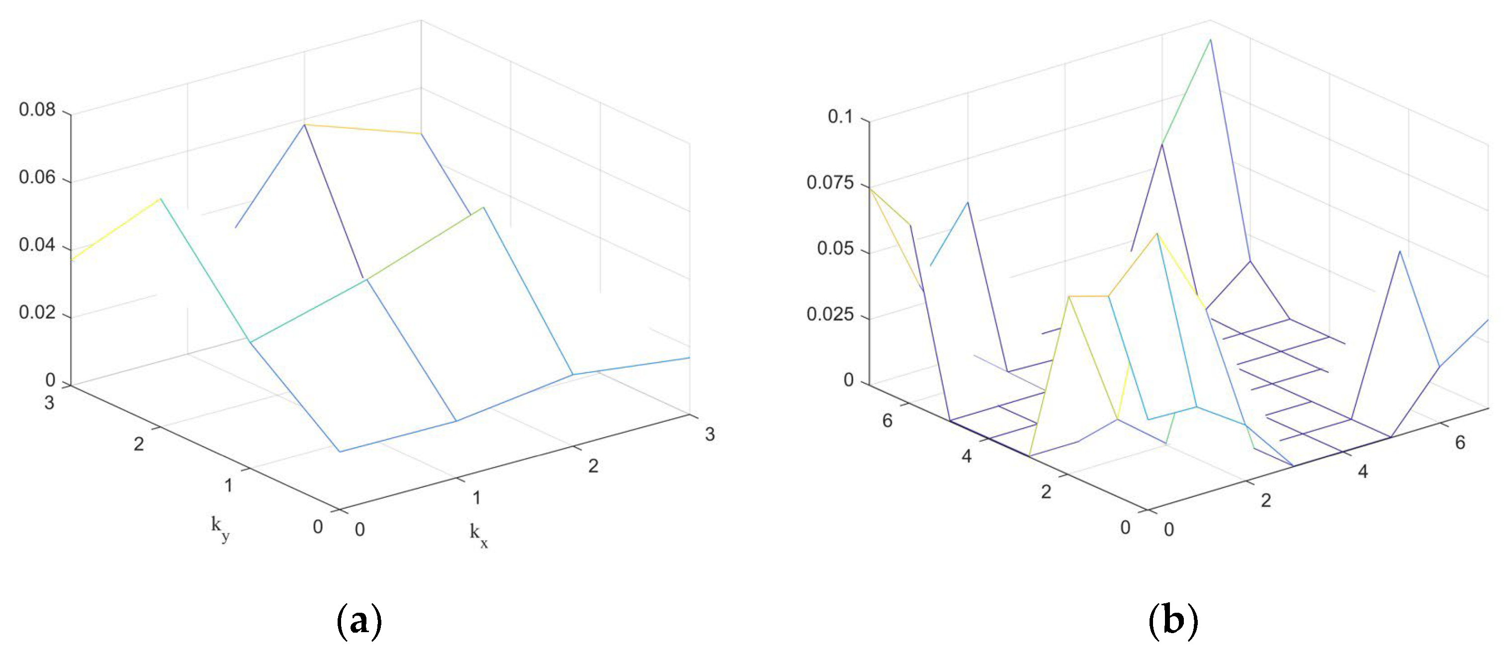
The corresponding angular spectrums of two-dimensional discrete data before and after smoothing are given below, as shown in Figure 5.

Through the analysis of the angular spectrum change in Figure 5, it can be found that the variation of each region is consistent with the variation law shown in Figure 3.

Table 3. Original angular spectrum value.

	ky	1	2	3	4
kx
1		0.017045	0.009228	0.021149	0.009228
2		−0.01436	0.040791	0.042617	0.009229
3		−0.06751	0.01527	−0.00131	0.01527
4		−0.01436	0.009229	0.042617	0.040791

and

Table 4. Regenerated angular spectrum value after smoothing.

	ky	1	2	3	4	5	6	7	8
kx
1		0.03409	0.018455	0.021149	0	0	0	0.021149	0.018455
2		−0.02872	0.081582	0.042617	0	0	0	0.042617	0.018458
3		−0.06751	0.01527	−0.00066	0	0	0	−0.00066	0.01527
4		0	0	0	0	0	0	0	0
5		0	0	0	0	0	0	0	0
6		0	0	0	0	0	0	0	0
7		−0.06751	0.01527	−0.00066	0	0	0	−0.00066	0.01527
8		−0.02872	0.018458	0.042617	0	0	0	0.042617	0.081582

list the angular spectrums before and after smoothing.

Now we analyze the variation of the angular spectrum in region A in line with Section 3.2. According to Table 3, the original angular spectrum value at (1, 1) in region A is 0.017045, and the regenerated angular spectrum value listed in Table 4 at the same position is 0.03409. This is in accordance with the principle that the angular spectrum value of the region A′ is twice that of the corresponding region A.

It can be seen from Table 3 that the original angular spectrum at (3,2) in region B is 0.01527. It can be seen from Table 4 that the position is divided into two positions after smoothing, which are (3,2) and (7,2), respectively. The generated angular spectrum value is 0.01527, which is the same as that of the corresponding region B.

It can be seen from Table 3 that the original angular spectrum at (3,3) in region C is −0.00131, and it can be seen from Table 4 that the smoothed position is divided into four regions, which are (3,3), (7,3), (3,7), and (7,7), respectively, and the generated angular spectrum value is −0.00066. This conforms to the principle that the value of the angular spectrum of region C’ is reduced to half of the value of the angular spectrum of region C.

It can be seen from Table 4 that the region D′ is the zero-padded region, and the generated angular spectrum values are all zeros. The above changes of angular spectrum are consistent with the theory given in Section 3.2, which can verify the correctness of the smoothing theory.

5. Twice Zero-Padding of Two-Dimensional Discrete Data

5.1. The First Zero-Padding of 16 × 8 Two-Dimensional Discrete Data

Much smoother results can be obtained through multiple zero-padding. Smoothing results of two-dimensional discrete data after one and two zero-paddings are given to illustrate this characteristic.

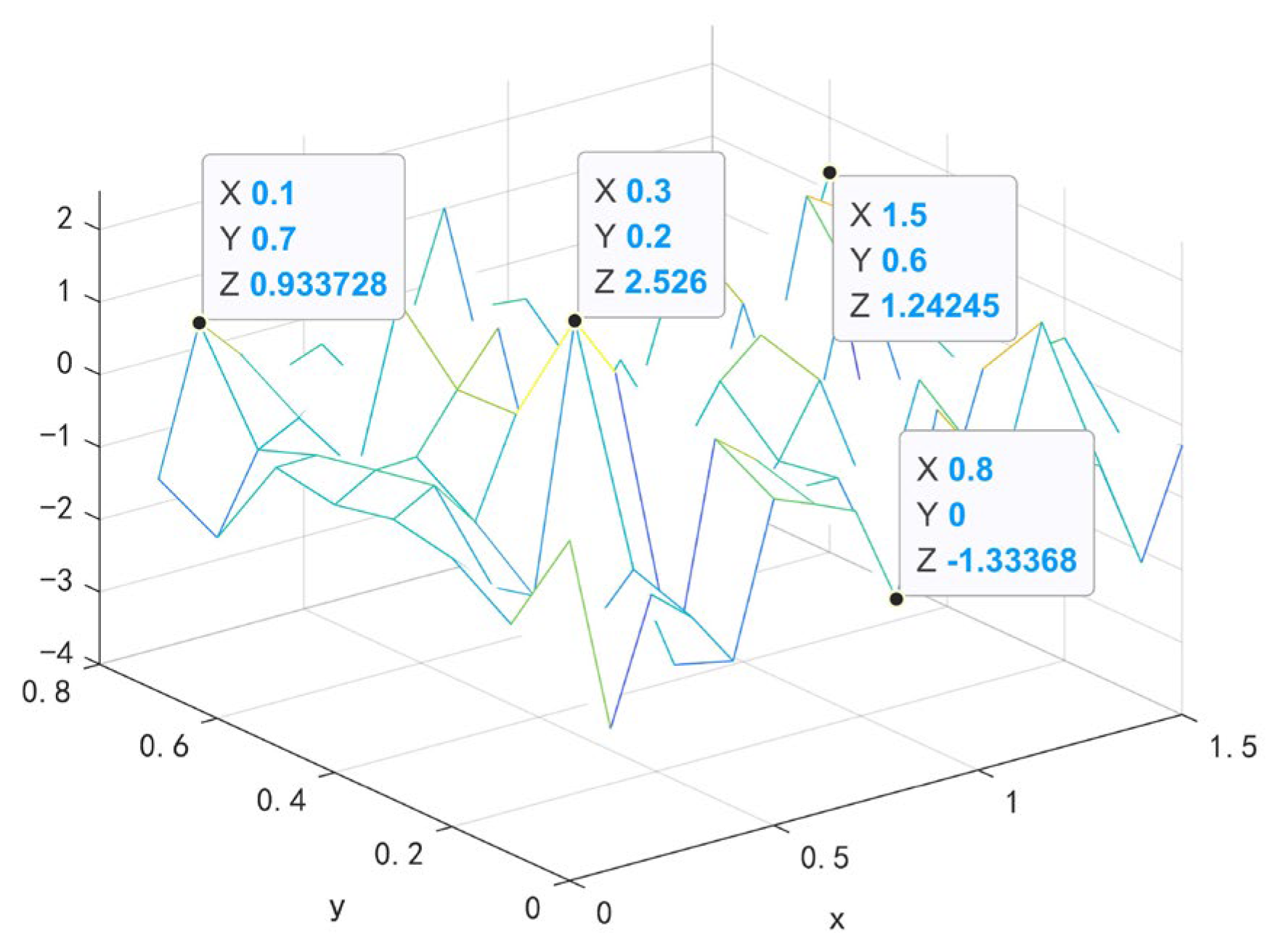
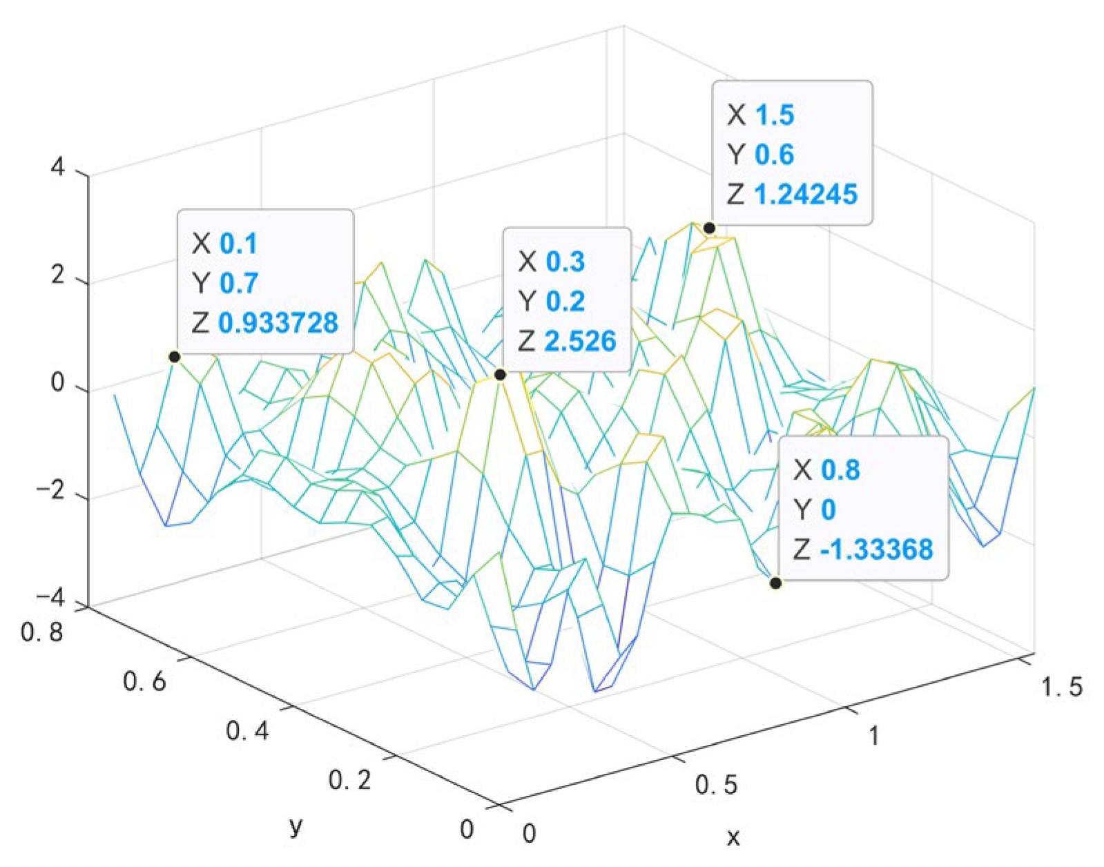
Figure 6 shows the known two-dimensional discrete data, which is randomly generated. Similarly, we assume that the sampling theorem is satisfied. The data numbers in x and y direction data are 16 and 8, respectively, and the spatial interval is 0.1 m. Test data values at four specific locations (0.1, 0.7), (0.3, 0.2), (0.8, 0), and (1.5, 0.6) are marked in Figure 6 for comparison with the smoothed results.

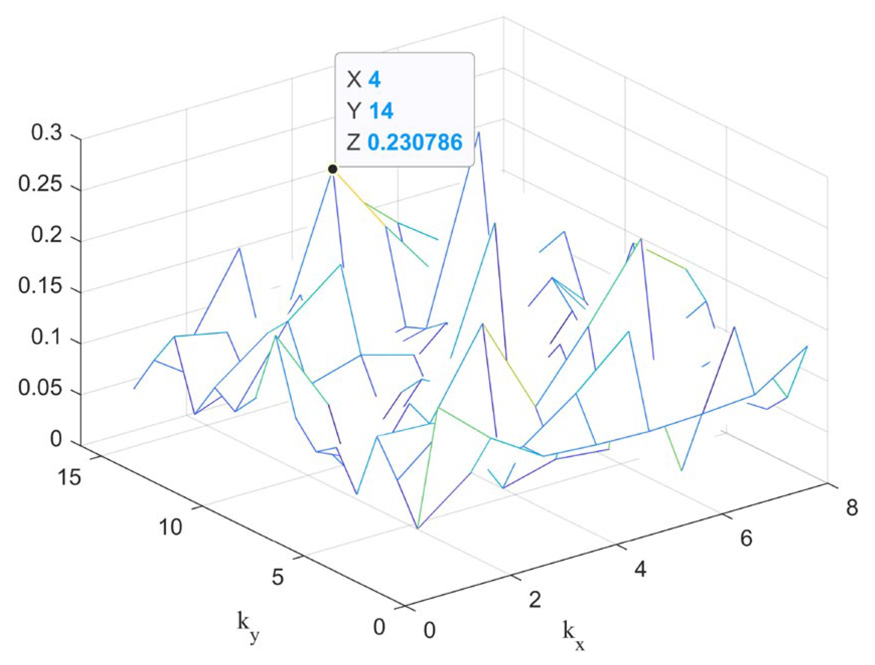
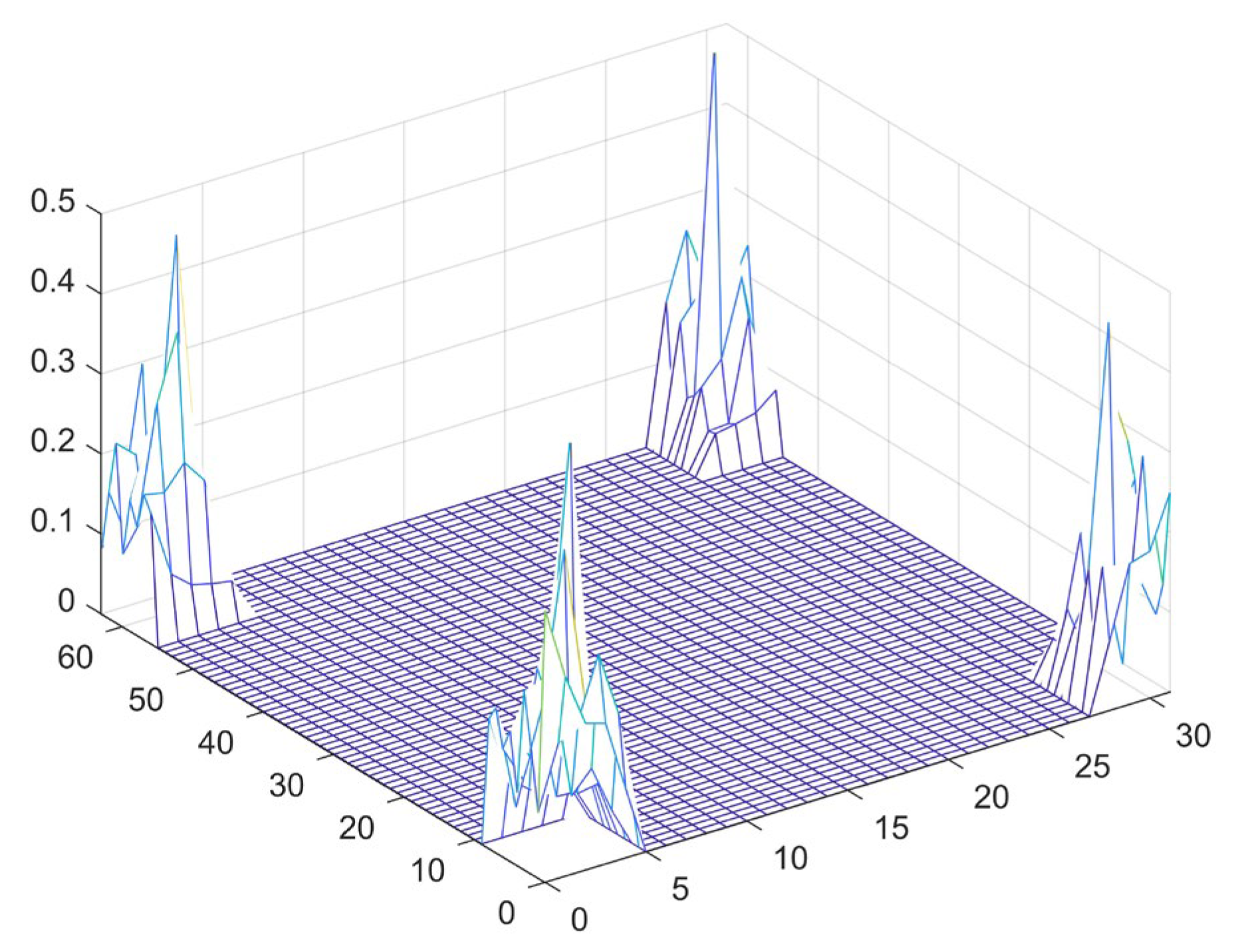
DFT is used to transform the original two-dimensional discrete data from the spatial domain to the wavenumber domain. Figure 7 shows the angular spectrum in the wavenumber domain after DFT.

To expand the sequence, the original angular spectrum is zero-padded, and the value of the angular spectrum at a particular location is modified. The angular spectrum after one zero-padding is the angular spectrum after smoothing once, as shown in Figure 8.

By comparing Figure 7 and Figure 8, it can be concluded that the variation of the angular spectrum of each region conforms to the smoothing theory shown in Figure 2 and Figure 3 in Section 3.2. For reasons of space, the angular spectrum values at each position are not listed here.

IDFT is applied to the angular spectrum after one zero-padding to produce two-dimensional discrete data after smoothing shown in Figure 9.

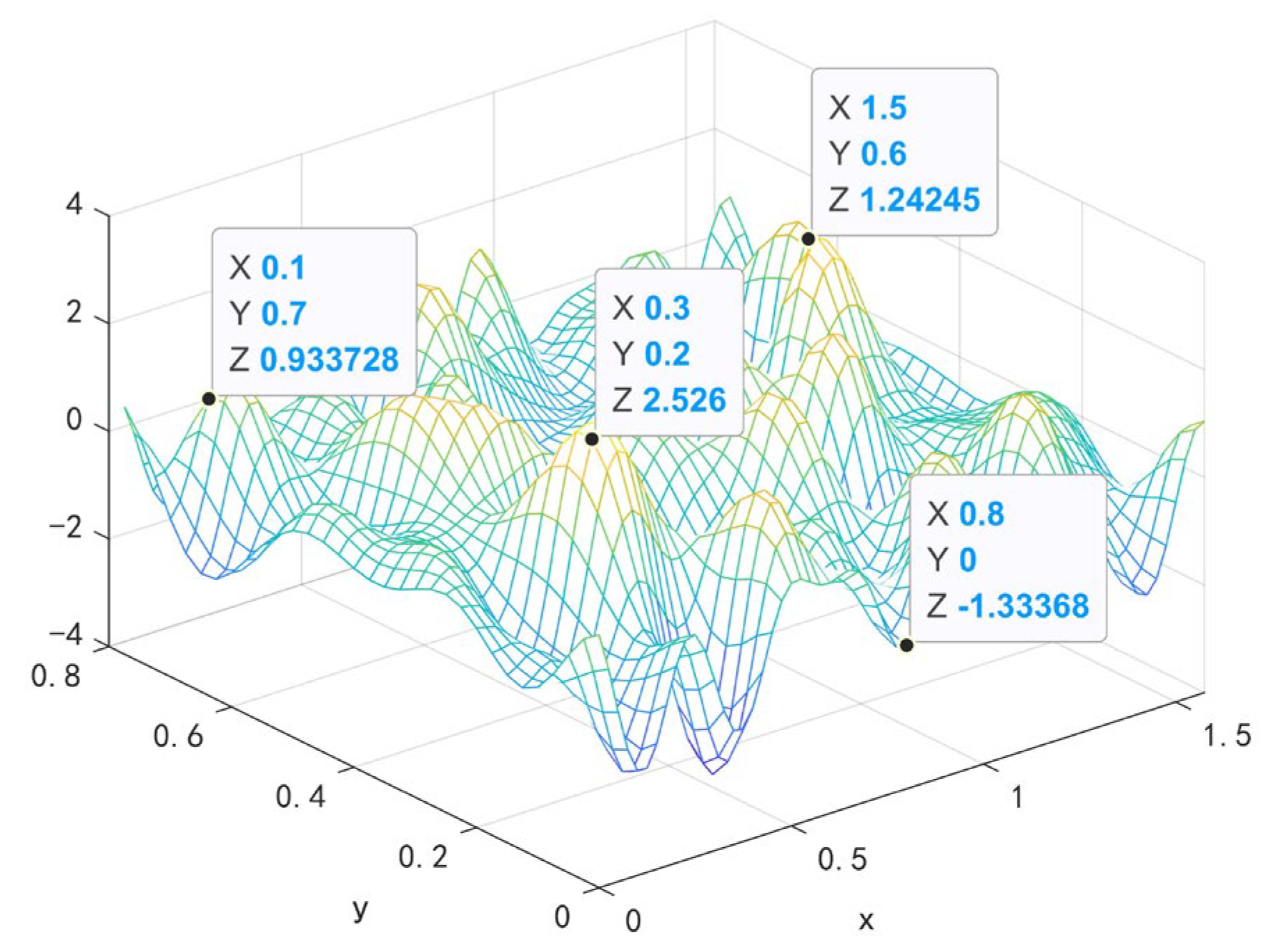
By comparing Figure 6 and Figure 9, it can be seen that the data density increases after smoothing. In Figure 9, the values at four specific locations (0.1, 0.7), (0.3, 0.2), (0.8, 0), and (1.5, 0.6) are also unchanged. The results verify the characteristics of increasing data density and constant values.

5.2. The Second Zero-Paddingof 16 × 8 Two-Dimensional Discrete Data

According to Figure 9, it is not difficult to find that the two-dimensional discrete data after one smoothing are relatively sharp in local areas. At this time, they can be smoothed again to achieve the purpose of data smoothing.

On the basis of one zero-padding, the new angular spectrum can be obtained by zero-padding again, as shown in Figure 10.

The angular spectrum after two zero-paddings is transformed by IDFT to obtain two-dimensional discrete data after twice smoothing, as shown in Figure 11.

A comprehensive comparison of Figure 6, Figure 9 and Figure 11 shows that the value of the discrete data after smoothing is unchanged. The data density increases, but there is some sharpness. After twice zero-padding, the value of discrete data is unchanged, the data density increases again, and the curve is relatively smoother.

The two-dimensional discrete data smoothing theory put forth in this paper is verified, as shown by the aforementioned numerical results. After the preceding zero-padding process, it is possible to verify that the method improves the density of the discrete data without changing the value size. In addition, the multiple computation feature of the smoothing theory for two-dimensional discrete data allows for the adjustment of data density to the proper level of computation.

6. Conclusions

This work proposes a two-dimensional discrete data smoothing method based on DFT and zero-padding in order to address the issue of limited test data in engineering practice.

• Firstly, the angular spectrum in wavenumber domain is obtained by DFT of the two-dimensional spatial discrete data. Then the angular spectrum is zero-padded and partially adjusted. Finally, IDFT is applied to obtain the smoothing results of two-dimensional discrete data. The proposed method is suitable for even rows or columns of sampling data.
• In this paper, the 4 × 4 two-dimensional discrete random data are smoothed, and the feasibility of the method is verified from the perspectives of numerical value and angular spectrum, respectively. From the numerical point of view, the smoothed two-dimensional discrete data are equal to the original data without changing the value of the data, indicating that the application of smoothing theory can achieve the desired effect. Smoothing results show the feasibility of smoothing theory.
• This paper also smoothed 16 × 8 two-dimensional discrete data twice, which shows that the smoothing theory of two-dimensional discrete data has the function of multiple calculations, and can adjust the data density to the appropriate degree of calculation.

In fact, the method can be extended to the smoothing of 3D discrete data and other areas related to data processing. Further studies can also focus on the adaptability of zero-padding and its practical application.

References

1. Chen, H.; Fan, L.; Wu, W.; Liu, H. Comparison of spatial interpolation methods for soil moisture and its application for monitoring drought. Environ. Monit. Assess 2017, 189, 525. [Google Scholar] [CrossRef] [PubMed]
2. Yao, L.; Wu, F.; Wu, G. Numerical study of exterior acoustic problems using a novel finite element-least square point interpolation method with perfectly matched layer. Eng. Anal. Bound. Elem. 2019, 102, 87–96. [Google Scholar] [CrossRef]
3. Sim, K.S.; Ting, F.F.; Leong, J.W.; Tso, C.P. Signal-to-noise ratio estimation for SEM single image using cubic spline interpolation with linear least square regression. Eng. Lett. 2019, 27, 151–165. [Google Scholar] [CrossRef] [Green Version]
4. Genya, K.; Shonosuke, S.; Yuki, K. Spatio-temporal Smoothing; Interpolation and Prediction of Income Distributions based on Grouped Data. arXiv 2022, arXiv:2207.08384. [Google Scholar]
5. Maier, L.B. Sparse Data Interpolation and Smoothing on Embedded Submanifolds. J. Sci. Comput. 2020, 84, 19. [Google Scholar] [CrossRef]
6. Wang, L.; Cheng, X.Q.; Xing, Z.Y. A fitting method for wheel profile line based on lagrange multiplier. Lect. Notes Electr. Eng. 2016, 378, 249–257. [Google Scholar] [CrossRef]
7. Amat, S.; Busquier, S.; Escudero, A.; Carlos, T.J. Lagrange interpolation for continuous piecewise smooth functions. Lect. Notes Electr. Eng. 2008, 221, 47–51. [Google Scholar] [CrossRef] [Green Version]
8. Mohammed, O.; Abdellah, L.; Mohamed, L.; Mhamed, M. Fitting and Smoothing Data Using Algebraic Hyperbolic Cubic Hermite Spline Interpolation. Eng. Lett. 2022, 30, 249–257. [Google Scholar]
9. Roman, D. Streaming Hermite interpolation using cubic splinelets. Comput. Aided Geom. Des. 2021, 88, 102011. [Google Scholar] [CrossRef]
10. Han, X.L.; Yang, J. A two-step method for interpolating interval data based on cubic hermite polynomial models. Appl. Math. Model. 2020, 81, 356–371. [Google Scholar] [CrossRef]
11. Han, X.; Guo, X. Cubic Hermite interpolation with minimal derivative oscillation. J. Comput. Appl. Math. 2018, 331, 82–87. [Google Scholar] [CrossRef]
12. Morelli, M.; Moretti, M.; D’Amico, A.A. Single-Tone Frequency Estimation by Weighted Least-Squares Interpolation of Fourier Coefficients. IEEE Trans. Commun. 2022, 70, 526–537. [Google Scholar] [CrossRef]
13. Wu, H.; Rui, D.; Song, L.H.; Yang, R.X.; Zhang, J.; Cao, J. Data processing method of noise logging based on cubic spline interpolation. Appl. Math. Nonlinear Sci. 2021, 6, 93–101. [Google Scholar] [CrossRef]
14. Aràndiga, F.; Baeza, A.; Yáñez, D.F. Monotone cubic spline interpolation for functions with a strong gradient. Appl. Math. Nonlinear Sci. 2022, 172, 591–607. [Google Scholar] [CrossRef]
15. Pang, Y.D.; Liu, H.J.; Zhou, C.M.; Huang, J.B.; Gu, H.C.; Zhang, Z.Q. Pretreatment of Ultra-Weak Fiber Bragg Grating Hydrophone Array Based on Cubic Spline Interpolation Using Intensity Compensation. Sensors 2022, 22, 6814. [Google Scholar] [CrossRef]
16. Wu, J.; Liu, K.P.; Le, J.; Wang, L.; Chen, Y.H. Harmonic analysis based on cubic spline interpolated arithmetic fourier transform. Lect. Notes Electr. Eng. 2015, 334, 259–269. [Google Scholar] [CrossRef]
17. Liu, G.M.; Wang, Y.J.; Zhang, H.R.; Wang, D. Comparative Study of Several Interpolation Methods in Spatial Analysis. Geogr. Inf. World 2011, 9, 41–45. [Google Scholar]
18. Domuta, I.; Palade, T.P. Sliding DFT and zero padding. In Proceedings of the 2019 42nd International Conference on Telecommunications and Signal Processing, Hungary, Budapest, 1–3 July 2019. [Google Scholar] [CrossRef]
19. Michal, L.; Andrzej, D.; Stefan, B. Active tone elimination algorithm using FFT with interpolation and zero-padding. In Proceedings of the Signal Processing: Algorithms, Architectures, Arrangements, and Applications, Poznan, Poland, 23–25 September 2020; Volume 9, pp. 163–168. [Google Scholar] [CrossRef]
20. Luo, J.F.; Xie, Z.J.; Xie, M. Interpolated DFT algorithms with zero padding for classic windows. Mech. Syst. Signal Process. 2016, 70–71, 1011–1025. [Google Scholar] [CrossRef]
21. Dai, S.K.; Zhang, Y.; Li, K.; Chen, Q.R.; Ling, J.X. Arbitrary Sampling Fourier Transform and Its Applications in Magnetic Field Forward Modeling. Appl. Sci. 2022, 12, 12706. [Google Scholar] [CrossRef]
22. Kan, Y.Z.; Zhu, Y.F.; Tang, L.; Fu, Q.; Pei, H.C. FGG-NUFFT-Based Method for Near-Field 3-D Imaging Using Millimeter Waves. Sensors 2016, 16, 1525. [Google Scholar] [CrossRef] [PubMed] [Green Version]
23. Kim, H.T.; Jin, K.C.; Kim, S.T.; Kim, J.; Choi, S.B. 3D Body Scanning Measurement System Associated with RF Imaging, Zero-padding and Parallel Processing. Meas. Sci. Rev. 2016, 16, 77–86. [Google Scholar] [CrossRef] [Green Version]
24. Xiang, J.Z.; Cui, W.; Shen, Q. Flexible and Accurate Frequency Estimation for Complex Sinusoid Signal by Interpolation Using DFT Samples. Chin. J. Electron. 2018, 27, 109–114. [Google Scholar] [CrossRef]
25. Veronesi, W.A.; Maynard, J.D. Nearfield acoustic holography (NAH) II. Holographic reconstruction algorithms and computer implementation. J. Acoust. Soc. Am. 1987, 81, 1307–1322. [Google Scholar] [CrossRef]
Figure 1. Block diagram of smoothing process for two-dimensional discrete data.
Applsci 13 04816 g001
Figure 2. Regional division of the original angular spectrum.
Applsci 13 04816 g002
Figure 3. Regional division of the generated angular spectrum.
Applsci 13 04816 g003
Figure 4. Original and regenerated two-dimensional data: (a) Original two-dimensional discrete data; (b) regenerated two-dimensional discrete data.
Applsci 13 04816 g004
Figure 5. Angular spectrums before and after smoothing: (a) Original angular spectrum; (b) regenerated angular spectrum.
Applsci 13 04816 g005
Figure 6. Original two-dimensional discrete data.
Applsci 13 04816 g006
Figure 7. The original angular spectrum.
Applsci 13 04816 g007
Figure 8. Generated angular spectrum after one zero-padding.
Applsci 13 04816 g008
Figure 9. Generated two-dimensional discrete data after first smoothing.
Applsci 13 04816 g009
Figure 10. Generated angular spectrum after second zero-padding.
Applsci 13 04816 g010
Figure 11. Generated two-dimensional discrete data after second zero-padding.
Applsci 13 04816 g011