Complement-Class Harmonized Naïve Bayes Classifier

Abstract

Naïve Bayes (NB) classification performance degrades if the conditional independence assumption is not satisfied or if the conditional probability estimate is not realistic due to the attributes of correlation and scarce data, respectively. Many works address these two problems, but few works tackle them simultaneously. Existing methods heuristically employ information theory or applied gradient optimization to enhance NB classification performance, however, to the best of our knowledge, the enhanced model generalization capability deteriorated especially on scant data. In this work, we propose a fine-grained boosting of the NB classifier to identify hidden and potential discriminative attribute values that lead the NB model to underfit or overfit on the training data and to enhance their predictive power. We employ the complement harmonic average of the conditional probability terms to measure their distribution divergence and impact on the classification performance for each attribute value. The proposed method is subtle yet significant enough in capturing the attribute values’ inter-correlation (between classes) and intra-correlation (within the class) and elegantly and effectively measuring their impact on the model’s performance. We compare our proposed complement-class harmonized Naïve Bayes classifier (CHNB) with the state-of-the-art Naive Bayes and imbalanced ensemble boosting methods on general and imbalanced machine-learning benchmark datasets, respectively. The empirical results demonstrate that CHNB significantly outperforms the compared methods.

1. Introduction

Machine learning (ML) is a data-driven approach that has emerged as a useful tool for rapid and accurate prediction. However, under-sampled or non-representative data can lead to incomplete information about a concept, making it difficult to make accurate predictions, causing overfitting problems. In overfitting, the ML model is over-optimized to the training data and fails to generalize unseen examples. This problem becomes worse if the data is high-dimensional or if the model has multiple tunable parameters, such as in deep learning or boosted models [1,2,3,4].

The challenges posed by scarce data have been recognized and extensively discussed in the research community for some time. In general, existing approaches apply data-level, model-level, or combined techniques that act in very different ways. For example, under-sampling, over-sampling [5], cleaning-sampling [6], or hybrid [7] are data-level methods that can deal with data scarcity. Recent research combines these resampling techniques with ensemble models because of the flexible characteristics of ensemble models, such as reducing prediction errors, and reducing bias and/or variance. Each phase of ensemble models provides a chance to make the model better for classifying the minority class by taking a base learning algorithm and training it on a different training set. Different algorithms using different resampling methods for building ensemble models were proposed [8,9,10,11]. SMOTE [5] is the most influential data-level technique for class-imbalance problems [12], which generates synthetic rare class samples based on the sample of k nearest neighbors with the same class. However, SMOTE and its variants have two main drawbacks in synthetic sample generation [13]; Rare classes’ probability distributions are not considered, and in many cases, the generated minority class samples lack diversity and overlap heavily with major classes.

Many recent published works addressed these drawbacks. Mathew et al. [13] proposed a weighted kernel-based SMOTE, which generates synthetic rare class samples in a feature space. The authors in [14] proposed a SMOTE-based, class-specific, extreme learning machine, which exploits the benefits of both the minority oversampling and class-specific regularization to overcome the limitation of the linear interpolation of SMOTE. In [2], a generalized Dirichlet distribution was used as a prior for the multinomial NB classifier to find non-informative generalized Dirichlet priors so that its performance on high-dimensional imbalanced data could be largely improved compared with generating synthetic instances in a high-dimensional space.

Naïve Bayes (NB) classifier is a well-known classification algorithm for high-dimensional data because of its computational efficiency, robustness to noise [15], and support of incremental learning [16,17,18]. This is not the case for other machine learning algorithms, which need to be retrained again from scratch. In the Bayesian classification framework, the posterior probability is defined as:

$$P\left(c|x\right)=\frac{P\left(x|c\right)P\left(c\right)}{P\left(x\right)}$$

(1)

where x is the feature vector, c is the classification variable, P(x) is the evidence, P(x|c) is the likelihood probability distribution, and P(c|x) is the posterior probability. However, we cannot obtain reliable estimates of the likelihood P(x|c) due to the curse of dimensionality. However, if we assume that, given a class label, each attribute is conditionally independent of each other and all attributes are equally important, then the computation of P(x|c) is made feasible and is obtained simply by multiplying the probability for each individual attribute, Equation (2).

$$P\left(x|c\right)=\prod _{j=1}^{m}P\left(x_j|c\right),$$

(2)

This is the core concept of Naive Bayes (NB) classifier which uses Equation (3) to classify a test instance (x), where $a_i$ is the i-th attribute value:

$$c\left(x\right)=\arg \underset{c\in C}{\mathrm{m}\mathrm{a}\mathrm{x}}P\left(c\right)\prod _{i=1}^{m}P\left(a_i|c\right)$$

(3)

Equation (3) is simple because the conditional independence assumption is made for efficiency reasons and to make it possible to estimate the values of all probability terms, since in practice, many attribute values are not represented in training data in sufficient numbers. However, the performance of NB degrades in domains where the independence assumption is not satisfied [19,20] or where the training data are scarce [21,22].

Various methods and approaches have been proposed to address the first problem and relax the attributes’ conditional independence assumption by extending NB structure [23,24], attribute selection [25,26], and attribute weighting methods [3,27,28,29,30,31,32,33,34]. To alleviate the second problem, other methods are proposed that act in very different ways on scarce data, such as instance cloning [35,36], instance weighting [37,38], and fine-tuning Naive Bayes [1,39]. However, to the best of our knowledge, most existing approaches for alleviating attributes’ conditional independence assumption and the data scarcity problem have one or both of the following problems: 1. Overfitting due to increased model complexity, especially on small or imbalanced datasets, 2. The absence of profound identification of potential discriminative attribute (feature) value in the presence of scant data. Consequently, the improvement of the enhanced NB classifier will be limited due to not targeting the right potential discriminative attributes for improving its representations in the data and its predictive power.

For example, current state-of-the-art attribute weighting [30,34,40] and fine-tuning [39] Naive Bayes classifiers are fine-grained boosting of attribute values, however, the complexity of the methods increases their tendency to overfit the training data and become less tolerant to noise [1,3,41]. In addition, the methods are either class-independent [30], where it assigns each attribute value the same weight for all classes, or class-dependent [34,39,40], but not considering the attribute value distribution divergence between different classes simultaneously. Thus, an attribute value that is equally distributed but highly correlated with two or more classes is considered a discriminative attribute and enjoys the highest attribute weights in case of attribute weighting or the largest probability term update amount in case of fine-tuning algorithms.

We proposed a new fine-tuning approach of NB; we call it the complement-class harmonized NB classifier (CHNB), which is different from the original fine-tuning algorithm FTNB [39] in capturing the attribute value inter-correlation (between classes) and intra-correlation (within the class). The aim is to improve the estimation of conditional probability and mitigate the effect of conditional independent assumption, especially for domains with scant and imbalanced data. In the proposed CHNB, the fine-tuning update amount is computed gradually to increase or decrease impacted probability terms, therefore, CHNB creates a more dynamic and accurate distribution for each rare class attribute value which would eliminate diversity and overlap the drawbacks of the synthetic sample generation of SMOTE and its variants. Moreover, CHNB can be integrated with any data-level approaches for class imbalanced problems, such as SMOTE.

We hypothesize that this approach will improve asymptotic accuracy, especially in domains with scarce data, without reducing the accuracy in domains with sufficient data. We conducted extensive experiments to compare our proposed method with state-of-the-art attribute weighting and fine-tuning NB methods on 41 general benchmark datasets, and with imbalanced ensemble methods on three imbalanced benchmark datasets.

The remainder of this paper is organized as follows. In Section 2, we review related work. In Section 3, we propose our CHNB algorithm. In Section 4, we describe the experimental setup and results in detail. In Section 5, we provide our conclusions and suggestions for future research.

2. Background and Related Work

Naïve Bayes (NB) classifier is efficient and robust to noise [15]. However, the performance of NB degrades in domains where the independence assumption is not satisfied [19,20] or where the training data are scarce [21,22]. Bayesian networks (BN) [42] eliminate the naïve assumption of conditional independence; however, finding the optimal BN is NP-hard [43,44]. Therefore, approximate methods that restrict the structure of the network [23,24,45] have been proposed to make it more tractable. Other methods attempt to ease the independence assumption by selecting relevant attributes [25,26,46]. The expectation here is that the independence assumption is more likely to be satisfied by a small subset of attributes than by the entire set of attributes. Attribute weighting is more flexible than attribute selection where it assigns a positive continuous value weight to each attribute. Attribute weighting is broadly divided into filer-based methods [27,28,29,30] or wrapper-based methods [3,32,33,34]. The former determines the weights in advance as a preprocessing step, using the general characteristics of the data, while the latter uses classifier performance feedback to determine attribute weights. Wrapper-based methods generally have better performance and are more complex than filter-based methods, but they are prone to overfit on small datasets [3].

In [33], attributes of different classes are weighted differently to enhance the discrimination power of the model as opposed to the general attribute weighting approach [32]. To improve the generalization capability of class-dependent attribute weighting [33], a regularized posterior probability is proposed [3], which integrates class-dependent attribute weights [33], class-independent attribute weights [32], and a hyperparameter in a gradient-descent-based optimization procedure to balance the trade-off between the discrimination power and the generalization capability. The experimental results validate the effectiveness of the proposed integrated method and demonstrate good generalization capabilities on small datasets [3]. However, attribute weighting methods [3,32,33] cannot estimate the influences of different attribute values of the same attribute. Therefore, Refs. [30,34] proposed a fine-grained attribute value weighting approach and assigned different weights to each attribute value.

Correlation-based attribute value weighting (CAVW) [30] is mainly determined by computing the attribute’s value-class correlation (relevance). The intuition is that the attribute value with maximum (relevance) is considered to be a highly predictive attribute value, and thus, will have higher weights. This assumption has a drawback of considering an attribute value that is equally distributed but highly correlated with two or more classes as a discriminative attribute, accordingly receiving a larger weight, where intuitively, a discriminative attribute should be highly correlated with a class, but at the same time, they are not correlated with other classes. On the other hand, class-specific attribute value weighting (CAVWNB) [34] provides greater discrimination, however, the model’s complexity is considerably increased, and the generalization capability is decreased due to the fine-grained boosting of attribute values [3]. The problem will be severe on a small dataset, causing an overfitting problem.

To alleviate the second problem of the NB classifier, namely, the scarcity of data, several methods were proposed to improve the estimation of probability terms. In [35,36], instance cloning methods were used to deal with data scarcity. In [35], a lazy method is used to clone instances based on their dissimilarity to a new instance, where in [36], a greedy search algorithm was employed to determine the instances to clone. These methods are lazy because they build the NB classifier during classification, therefore, the classification time is relatively high [47]. The Discriminatively Weighted Naïve Bayes (DWNB) [37] method assigns instances different weights depending on how difficult they are to classify. In [48], the probability estimation problem was modeled as an optimization problem and metaheuristic approaches were used to find a better probability estimation. FTNB [39] was proposed to address the problem of data scarcity for the NB classifier. However, the fine-tuning procedure in FTNB [39] leads to overfitting problems and makes NB less tolerant to noise, therefore, a more noise tolerant FTNB was proposed in [1] and also, a FTNB combined with instant weighting was proposed in [41].

Despite the enhancements of FTNB [1,39,41], the fine-tuning procedure is similar to correlation-based attribute weighting methods [27,29,30] where calculating the update amount (weight) does not simultaneously incorporate the inter-correlation (between classes) distance measure for each attribute value. More specifically, Information gain $IG\left(C\right|a_{ij})$ is used to measure the difference between a priori and a posteriori entropies of a class target, C, given the observation of feature a, and intuitively, a feature with higher information gain deserves a higher weight [27]. However, in [27], the author proposed the Kullback–Leibler Measure (KL) Equation (4) as a measure of divergence and as the information content of a feature value $a_{ij}$ to overcome the possible zero or negative values’ limitations of IG as a feature weighting.

$$\mathrm{K}\mathrm{L}\left(C\mid a_{ij}\right)=\sum _{c}P\left(c\mid a_{ij}\right)\log \frac{P\left(c\mid a_{ij}\right)}{P\left(c\right)}$$

(4)

where $a_{ij}$ corresponds to the j value of the i-th feature in training data. Thus, the weight of a feature can be defined as the weighted average of the KL measures across the feature values. $\mathrm{K}\mathrm{L}\left(C\mid a_{ij}\right)$ and mutual information $\mathrm{M}\mathrm{I}\left(C\mid a_{ij}\right)$ Equation (5) are employed in [29,30] as two different base methods to measure the significance (relevance) between each attribute value and class target and consequently, the attribute value weights for the NB classifier.

$$I\left(a_i;C\right)=\sum _{c}P\left(a_i,c\right)\log \frac{P\left(a_i,c\right)}{P\left(a_i\right)P\left(c\right)}.$$

(5)

The expectation is that a highly predictive attribute value should be strongly associated with class (maximum attribute value mutual relevance) [30]. In FTNB [39], every misclassified training instance is fine-tuned by updating its conditional probability terms of actual (ground truth label) and predicted classes. In FTNB [39], conditional probability terms of actual class are increased by an amount that is proportional to the difference between $p\left(a_j|c_{actual}\right)$ and $P_{max}\left(a_j|c_{actual}\right)$, and contrarily, the conditional probability terms of predicted class decreased by an amount that is proportional to the difference between $p\left(a_j|c_{predicted}\right)$ and $P_{min}\left(a_j|c_{predicted}\right)$, using Equations (6) and (7), respectively.

$${\delta }_{t+1}\left(a_j,c_{actual}\right)=\eta ·\left(\alpha ·P_{max}\left(a_j|c_{actual}\right)-p\left(a_j|c_{actual}\right)\right)·error$$

(6)

$${\delta }_{t+1}\left(a_j,c_{predicted}\right)=-\eta ·\left(\alpha ·p\left(a_j|c_{predicted}\right)-P_{min}\left(a_j|c_{predicted}\right)\right)·error$$

(7)

where $\eta$ is a learning rate between zero and one, used to decrease the update step, and $\alpha$ is constant = 2, and error is the general difference between the two posteriors of the actual and predicted classes. The fine-tuning process will continue as long as training classification accuracy keeps improving.

There is a fundamental problem with correlations measures (KL) Equation (4) (MI), Equation (5), and (FTNB) Equations (6) and (7) where they would consider a relatively equally distributed but highly correlated attribute value with two or more classes as a discriminative attribute value. Thus, the update amount (weight) for the attribute value will be substantially large to boost its discriminative power. However, discriminative attributes should be highly correlated with a class, but at the same time, should not be correlated with other classes. Therefore, the discriminative power of attribute values should correspond to the amount of divergence between the attribute value’s conditional probability distributions of different classes, and its update amount (weight) is proportional to the distance measure of the divergence.

In this paper, we propose a subtle yet significant enough discriminative attribute value boosting for the Naïve Bayes classifier to reliably estimate its probability terms. The aim is to boost the discriminative attribute value (and more importantly, the hidden discriminative attribute value) to improve its predictive power influence on classifying the correct target class. Despite that the relationship between attribute values and class prediction may be highly and globally non-linear, the local linear relationship defined in our proposed method for discriminative attribute values is more than powerful enough for boosting the Naïve Bayes classifier, given its conditional independence assumption. Moreover, the aim, as we will see next, is to identify potentially hidden discriminative attribute values for substantial boosting to increase its predictive power in the presence of scant data. In this paper, which is an extension of our previous work [4], we further investigate the following:

-

The proposed method is compared with state-of-the-art attribute weighting methods on 41 general benchmark datasets, and with relatively new state-of-the-art ensemble methods designed specifically for imbalanced datasets on three imbalanced benchmark datasets;

-

We modified the original FTNB [39] early termination condition in order to have a fair performance evaluation on imbalanced datasets;

-

Finally, we combine NB and the proposed method with different data-level resampling strategies to evaluate the performance on imbalanced datasets.

3. Complement-Class Harmonized Naïve Bayes Classifier (CHNB)

Fine-grained attribute value boosting of Naïve Bayes generally yields a better performance than general attribute boosting methods, but it is more likely to overfit on training datasets due to the increased complexity of the model and the schema of identifying discriminate attributes values. In our proposed method, we define three scenarios of attribute values’ conditional probability terms distribution. In the first scenario, a potential discriminative attribute value, ${Da}_{ij}$, might be under-represented in the training data. In this sense, the conditional probability term $P\left({Da}_{ij}\right|C)$ for both the ground truth label and other class labels will be substantially small due to non-representative data and a weak correlation between the ground truth label and other classes, respectively. We call such an attribute value a hidden discriminative attribute value, which leads to incomplete information, hence causing an underfitted model, which will generate a high misclassification rate in both training and testing data. Therefore, we should significantly boost misclassified instance attribute values that have small conditional probability terms $P\left({Da}_{ij}\right|C)$ in both predicted and actual classes.

In the second scenario, some potential discriminative attribute values might be under-sampled due to class-imbalanced datasets where many examples belong to one or more major classes, and few belong to minor classes. In this scenario, some discriminative attribute values (${Da}_{ij}$) would be hidden or considered as noise examples, which leads to an overfitting problem due to the bias toward major classes compared with the rare classes. It is very important to differentiate these examples from the third scenario’s examples that are strongly correlated with both classes. The former examples are affected by the under-sampling problem, which is very common in real-world applications, whereas the latter should be considered redundant information with no predictive power, given its relatively highly correlations with the different classes and not being impacted by the scant data problem.

In order to address these three different scenarios, we can apply disproportional probability term updates for misclassified instance attributes values, utilizing the harmonic average, since it is dominated by the smaller values. Precisely, for scenario 1, the complement harmonic average (1- harmonic average) would be large and the update size would be large for misclassified instance’s attributes values if both the $p\left(a_i|c_{actual}\right)$ and $p\left(a_i|c_{predicted}\right)$ were to be small. Similarly, for scenario 2 of skewed data, the complement harmonic average would be relatively large, and the update size would be large if either $p\left(a_i|c_{actual}\right)$ or $p\left(a_i|c_{predicted}\right)$ were to be small. Finally, in scenario 3, the complement harmonic average would be small, and the update size would be small if both the $p\left(a_i|c_{actual}\right)$ and $p\left(a_i|c_{predicted}\right)$ were to be large. Thus, in CHNB, we calculate the update weights for the $p\left(a_i|c_{actual}\right)$ and $p\left(a_i|c_{predicted}\right)$ of misclassified instances using Equations (8)–(10), respectively.

$$W_i=\frac{\eta }{t}·\left(1-2/(\frac{1}{p_t\left(a_i{|c}_{actual}\right)}+\frac{1}{p_t(a_i{|c}_{predicted})})\right)$$

(8)

$$p_{t+1}\left(a_i{|c}_{actual}\right)=p_t\left(a_i{|c}_{actual}\right)+W_i$$

(9)

$$p_{t+1}(a_i{|c}_{predicted})=p_t(a_i{|c}_{predicted})-W_i$$

(10)

Here, (η) is a learning rate between zero and one, and (t) is the iteration (epochs) number used as weight decay.

Contrary to what was reported in [39], in our case, it is useful to update the priors for misclassified instances when we have imbalanced training data. To modify class probability $p\left(c_{actual}\right)$ and $p\left(c_{predicted}\right)$ for misclassified instances, we apply Equations (11)–(13), respectively.

$$W_j=\frac{\eta }{t^2}·\left(1-2/(\frac{1}{p_t\left(c_{actual}\right)}+\frac{1}{p_t\left(c_{predicted}\right)})\right)$$

(11)

$$p_{t+1}\left(c_{actual}\right)=p_t\left(c_{actual}\right)+W_j$$

(12)

$$p_{t+1}\left(c_{predicted}\right)=p_t\left(c_{predicted}\right)-W_j$$

(13)

Thus, and since we modify the probability terms, one can think of them as fine-grained, class-dependent attribute value weighting. We tested our hypothesis in the next section on more than 40 general UCI datasets and three benchmark imbalanced datasets. We argue that applying this heuristic rule does not contradict any evidence observed in the training data, since the model is misclassifying training examples by underfitting or overfitting as identified in scenarios 1 and 2, respectively, and we can safely assume that there is no sufficient data to support the accurate classification of these training instances. The CHNB algorithm is briefly described as Algorithm 1.

Algorithm 1: CHNB fine tuning algorithm

Input: a set of training instances, D, and the maximum number of iterations, T.

Output: Fine-Tuned Naïve Bayes

Build an initial naïve Bayes classifier using D

t = 0

While the training F-score is improving and t < T do

a. For each training instance, inst, do

i. $\mathrm{c}\mathrm{l}\mathrm{a}\mathrm{s}\mathrm{s}\mathrm{i}\mathrm{f}\mathrm{y}\left(\mathrm{i}\mathrm{n}\mathrm{s}\mathrm{t}\right)$

ii. if $c_{predicted}<>c_{actual}$ //inst is misclassified

iii. for each attribute value, $a_i$, of inst Do

1. $p_{t+1}\left(a_i{|c}_{actual}\right)=p_t\left(a_i{|c}_{actual}\right)+W_i$

2. $p_{t+1}(a_i{|c}_{predicted})=p_t(a_i{|c}_{predicted})-W_i$

3. $p_{t+1}\left(c_{actual}\right)=p_t\left(c_{actual}\right)+W_j$

4. $p_{t+1}\left(c_{predicted}\right)=p_t\left(c_{predicted}\right)-W_j$

b. Let t = t + 1

4. Experimental Setup and Results

The proposed CHNB method was evaluated in two groups of experiments. First, CHNB was compared with related state-of-the-art methods on general purpose datasets. Secondly, we compared CHNB on imbalanced benchmark datasets with other related work. CHNB was tested using two sets of experiments and the objective was to evaluate the effectiveness of the proposed methods on both balanced and imbalanced datasets. In addition, we modified the termination condition of the original FTNB algorithm to be based on an F-score, similar to CHNB, instead of accuracy, for imbalanced dataset comparisons.

We implemented NB, FTNB, and the proposed CHNB classifiers in Java by extending the Weka source code of the Multinomial Naïve Bayes [49]. All continuous attributes were discretized using Fayyad et al.’s [22] supervised discretization method, as implemented in Weka [49], and missing values were simply ignored. We used stratified 10-fold cross-validation to evaluate the classification performance of the proposed algorithm on each dataset.

4.1. Comparison to State-of-the-Art (General Datasets)

In this section, the performance of the proposed method is compared with attribute weighting NB classifiers’ wrapper-based methods (WANBIA^CLL, CAWNB^CLL, and CAVWNB^CLL), filter-based methods (CAVW^MI), fine tuning naïve base (FTNB), combined filter-based and fine-tuning method (FTANB), and the original NB algorithm. The related work methods and their abbreviations are listed in

Table 1. Description of the competitors’ NB classifiers.

WANBIACLL	Attribute weighting NB with gradient based optimization on conditional log likelihood (CLL) [32]
CAWNBCLL	Class-specific Attribute weighting NB with gradient based optimization on (CLL) [33]
CAVWNBCLL	Class-specific Attribute value weighting NB with gradient based optimization on (CLL) [34]
CAVWMI	Filter method, correlation-based attribute value weighting measured by Mutual Information (MI) [30]
FTNB	Fine tuning naïve Bayes [39]
FTANB	Initial attribute weighted based on CAVWMI, then fine-tuned with FTNB algorithm [40]
NB	Base line multinominal NB
CHNB	Complement-class fine tuning naïve Bayes (ours)

.

Comprehensive experiments were conducted on 41 benchmark datasets obtained from the UCI repository [50]. Most datasets were collected from real-world problems, which represent a wide range of domains and data characteristics. The number of attributes/classes of these datasets varies, and hence, these datasets are diverse and challenging.

Table 2. UCI general dataset description.

Dataset	Instance	Attributes	Classes	Missing Values
Anneal	898	39	6	Y
Anneal.Orig	898	39	6	Y
Audiology	226	70	24	Y
Autos	205	26	7	Y
Breast-cancer	286	10	2	Y
Breast-w	699	10	2	Y
Car	1728	7	4	N
Colic	368	23	2	Y
Colic.ORIG	368	28	2	Y
Credit-a	690	16	2	Y
Credit-g	1000	21	2	N
Cylinder.bands	540	41	2	Y
Diabetes	768	9	2	N
Ecoli	336	8	8	N
Glass	214	10	7	N
Heart-c	303	14	5	Y
Heart-h	294	14	5	Y
Heart.statlog	270	14	2	N
Hepatitis	155	20	2	Y
Hypothyroid	3772	30	4	Y
Ionosphere	351	35	2	N
Iris	150	5	3	N
KR-vs.-KP	3196	37	2	N
Labor	57	17	2	Y
Letter	20,000	17	26	N
Lymph	148	19	4	N
Mushroom	8124	23	2	Y
Optdigits	5620	63	10	N
Page.blocks	5473	11	5	N
Pendigits	10,992	17	10	N
Primary-tumor	339	18	21	Y
Segment	2310	20	7	N
Sick	3772	30	2	Y
Sonar	208	61	2	N
Soybean	683	36	19	Y
Splice	3190	62	3	N
Vehicle	846	19	4	N
Vote	435	17	2	Y
Vowel	990	14	11	N
Waveform	1000	41	3	N
Zoo	101	18	7	N

shows the properties of these data sets.

Table 3. Classification performance (Accuracy) comparison results on 41 UCI general datasets.

Dataset	CHNB	NB		FTNB		CAVWNBCLL		CAVWMI		CAWNBCLL		WANBIACLL		FTANB
Anneal	99.11	95.77	●	98.00		99.23		97.62		98.60		98.00		97.97
Anneal.Orig	98.22	95.99	●	97.22		91.76	●	89.84	●	91.06	●	90.89	●	91.55	●
Audiology	76.17	72.23		73.40		77.02		75.78		82.10		78.08		75.81
Autos	85.38	74.76	●	82.45		75.94		68.38		75.08		74.98		70.00
Breast-cancer	62.98	73.08	○	62.22		68.57		72.14		69.53		71.00		72.01
Breast-w	96.57	97.28		96.71		96.07		97.28		96.20		96.88		97.14
Car	93.23	85.24	●	92.42		90.12		70.79	●	86.69	●	85.69	●	89.52	●
Colic	83.17	79.62		78.26		79.90		82.18		81.39		82.69		81.75
Colic.ORIG	75.01	73.09		76.37		75.95		74.40		76.77		74.26		74.62
Credit-a	84.93	86.09		84.06		84.14		86.01		85.28		85.29		85.41
Credit-g	71.40	75.80	○	69.70		74.94		75.53		75.48		76.13		76.09
Cylinder.bands	80.74	77.96		80.19		81.28		81.09		77.81		78.89		80.65
Diabetes	75.12	76.95		73.70		75.14		75.32		75.88		76.15		76.22
Ecoli	85.17	86.05		85.73		83.60		82.26		83.93		83.75		82.77
Glass	75.22	74.31		75.69		59.41		58.70		59.06		59.87		58.29
Heart-c	84.47	84.47		83.15		80.97		81.23		81.29		82.18		84.00
Heart-h	85.75	84.39		83.32		82.15		82.79		83.34		84.22		83.45
Heart.statlog	84.44	83.33		82.59		81.78		82.30		82.26		82.96		83.78
Hepatitis	87.79	87.83		87.08		83.09		85.86		84.95		84.35		85.16
Hypothyroid	99.20	98.30	●	99.18		93.50	●	93.53	●	93.53	●	93.58	●	93.39	●
Ionosphere	92.59	91.16		92.02		91.23		91.09		91.83		91.82		91.08
Iris	96.67	96.67		96.00		95.33		93.67		96.47		96.60		95.53
KR-versus-KP	97.21	87.70	●	96.09		95.08		90.21	●	94.31	●	93.43	●	94.70
Labor	92.33	92.33		92.33		94.60		93.33		94.07		93.80		92.80
Letter	84.40	74.11	●	78.08	●	77.64	●	67.89	●	71.25	●	68.42	●	72.90	●
Lymphography	84.52	85.24		82.38		84.05		83.67		82.37		84.09		83.95
Mushroom	99.99	95.78	●	99.93		99.82		97.07		99.80		99.69		99.85
Optdigits	95.62	92.38	●	95.00		95.08		92.48	●	95.62		93.94		94.68
Page.blocks	96.73	93.59	●	96.24		93.87	●	92.32	●	93.16	●	92.77	●	92.61	●
Pendigits	96.32	87.97	●	95.01	●	97.19		87.54	●	93.47	●	88.55	●	94.75	●
Primary-tumor	43.09	50.47		43.41		48.26		47.29		46.11		47.52		46.00
Segment	95.37	91.77	●	94.24		93.99		90.25	●	92.75		92.48		91.52
Sick	97.32	97.19		95.63		97.71		97.47		97.70		97.38		97.52
Sonar	85.04	85.12		84.57		77.63		75.33		76.66		75.56		76.09
Soybean	92.68	92.83		92.68		93.96		93.68		94.45		93.92		93.47
Splice	94.55	95.39		94.36		95.03		96.03		96.20		96.05		95.97
Vehicle	71.63	63.59	●	69.49		70.96		61.27	●	64.65		64.43		65.01
Vote	94.49	90.11	●	94.02		95.84		90.67		95.81		95.56		94.09
Vowel	82.63	66.57	●	69.49	●	82.19		68.35	●	71.30	●	70.34	●	71.39	●
Waveform-5001	84.30	80.76	●	82.38	●	85.29		79.75		83.30		81.39		82.27
Zoo	93.09			93.09		96.44		96.25		95.35		96.03		96.35
Average	86.69	84.55		85.31		85.26		82.89		84.56		84.23		84.44
W/T/L		2/23/16		0/37/4		0/37/4		0/30/11		0/33/8		0/33/8		0/35/6

● CHNB (ours) is significantly better. ○ CHNB (ours) is significantly worse.

shows the detailed classification accuracy obtained by averaging the results from stratified 10-fold cross-validation. The results of CAVWNB^CLL, CAWNB^CLL, and WANBIA^CLL were obtained from [34]. The results of CAVW^MI and FTANB were obtained from [30,40], respectively. The overall classification average result and the Win/Tie/Lose (W/T/L) values are summarized at the bottom of the table in addition to the other statistics. Each entry’s W/T/L in the table implies that the competitor wins on W datasets, ties on T datasets, and loses on L datasets compared with the proposed method. The field marked with ● and ○ implies that the classification accuracy of CHNB has statistically significant upgrades or degrades, respectively, compared with the competitor algorithm. We employed a paired tow-tailed t-test with a p = 0.05 significance level.

In Table 3, the result clearly reveals that the proposed CHNB has the highest average classification accuracy. Compared with the original Naive Bayes and FTNB, the proposed CHNB achieves, on average, 2.14% and 1.38% of improvement, respectively. Compared with the class-dependent attribute weighting approach, CAVWNB^CLL and CAWNB^CLL, the proposed CHNB achieves 1.43% and 2.13% of improvements on average, respectively. Compared with the class-independent attribute weighting approach, CAVW^MI and WANBIA^CLL, CHNB achieves 3.80% and 2.46% of improvements on average, respectively. Compared with the most recent algorithm, using the fine-tuning attribute-weighted method FTANB, the proposed CHNB achieves more than 2% of improvement for average classification accuracy over the 41 datasets. Among them, the improvements on some datasets are significant. For example, the classification accuracies of CHNB on Anneal.Orig, Autos, Glass, Letter, and Sonar are more than five times higher than the best attribute-weighting method, CAVWNB^CLL, and the most recent fine-tuning attribute-weighted method, FTANB.

On relatively small datasets, the proposed approach outperforms CAVWNB^CLL and FTANB on 8 out of the 10 smallest datasets because of the simplicity and good generalization capability of CHNB. On relatively large datasets, such as Letter and Mushroom, the proposed CHNB shows statistically significant improvements and CHNB performs the best compared with all other methods. The classification accuracy for CHNB on the Mushroom dataset is 99.99 while for example, NB and CAVW are 95.78 and 97.07, respectively. All these demonstrate that the proposed approach hardly overfits and very well generalizes different sizes of datasets.

For the statistically significant tests shown in Table 3, the proposed CHNB method outperforms all other methods. CHNB significantly outperformed NB and FTNB on 16 datasets, while significantly losing on only two datasets. Compared with the best attribute-weighting method, CAVWNB^CLL, and the most recent fine-tuning attribute-weighted method, FTANB, CHNB significantly outperformed on four and six datasets, respectively, and did not lose significantly on any datasets. Compared with general (non-fine-grained) attribute weighing methods (CAWNB^CLL and WANBIA^CLL), CHNB significantly outperformed on eight datasets for each method, while not significantly losing on any dataset. In addition, our proposed method, CHNB, shows a consistent performance across the 10-fold with low variance compared with competitors. For example, other methods, such as CAWNB^CLL and WANBIA^CLL, achieve, on average, ~10% improvements on the Breast-cancer dataset, however, their 10-fold results have large variance, and they are not significantly better than our method. In this dataset, our proposed method, CHNB, achieves (62.98 ± 2.54) in accuracy compared with NB (73.08 ± 2.42), CAVW^MI (72.14 ± 7.49), CAWNB^CLL (69.53 ± 7.37), WANBIA^CLL (71.00 ± 7.41), and FTANB (72.01 ± 7.69).

Noteworthy, a dataset with a relatively large number of attributes and classes contributes more to the significant improvement of CHNB compared with attribute weighting methods. This observation is expected given that attribute weighting methods are tailored to alleviate class-independent assumption problems as discussed earlier. Therefore, independence assumption is more likely to be satisfied in datasets with a relatively small number of attributes, hence reducing the chance of significant improvement between algorithms. Specifically, our proposed method significantly outperforms other competitors on datasets with a large number of attributes, such as Anneal.orig, Hypothyroid, KR-vs.-KP, Letter, and Mushroom datasets. Moreover, we can see that some of the UIC datasets above are Imbalance and F-score or other metrics that are suitable for a class-imbalance dataset that should be reported instead of accuracy. It can also be seen that the proposed CHNB indeed demonstrates good generalization capabilities on general datasets. In the next experiment, we will verify the performance gain of the proposed method on imbalanced multi-class benchmark datasets.

4.2. Comparing the Methods (Imbalanced Datasets)

In the imbalanced datasets’ evaluation, we changed the early termination condition for the original FTNB to be based on F-score instead of accuracy. We also compare our work with four state-of-the-art ensemble approaches especially designed for dealing with imbalanced datasets, namely, BalancedBagging [8], BalancedRandomForest [9], RUSBoost [10], and EasyEnsemble [11]. We used the imbalanced-learn Python package [51] to implement the ensemble methods using the methods’ default hyperparameters. We evaluated the proposed method with respect to F-score since it is a more suitable evaluation criterion than accuracy for imbalanced datasets. We used 10-fold cross-validation and a paired two-tailed t-test with 95% confidence to evaluate the classification performance on each dataset. Multi-class confusion matrices were built for each dataset to calculate the macro average (unweighted) F-score. Thus, major and minor classes would equally contribute to the measurement metrics. In addition to F-score, we used Cohen’s kappa and Matthew’s correlation coefficients to overcome the limitations of the F-score metric which does not take the false positive rate into account. Cohen’s kappa makes a better evaluation of the performance on multi-class datasets, where it measures the agreement between the predictions and ground truth labels, while MCC measures all the true/false positives and negatives. Both metrics’ (kappa and MCC) scores ranged between −1 and 1, and values greater than 0.8 were considered as strong agreement [52].

Table 4. Imbalanced datasets summary.

Dataset	Instance	Attributes	Classes	LRID	Class Distribution (%)
CIC-IDS 2017 [55]	2,830,743	83	14	3.88	(80.3, 8.2, 5.6, 4.5, 0.4, 0.3, 0.2, 0.2, 0.2, 0.1, 0.1, 0.0, 0.0, 0.0, 0.0)
Ransomware [56]	1524	30,967	11	1.99	(61.8, 7.0, 6.4, 5.9, 4.2, 3.9, 3.3, 3.0, 2.2, 1.6, 0.4, 0.3)
WSN [57]	374,661	19	4	2.3	(90.8, 3.9, 2.7, 1.8, 0.9)

shows a brief description of three benchmark class-Imbalance datasets with their Imbalance degrees [53]. The datasets have a multi-minority problem (more than one minor class) and previous studies have shown that multi-minority problems are harder than multi-majority problems [53,54]. The first dataset, created by the Canadian Institute for Cybersecurity (CIC), was to be used as a benchmark dataset to evaluate intrusion detection systems [55]. The CIC-IDS’17 dataset [55] contains both raw and aggregated netflow data of the most up-to-date common attacks. The dataset contains five categorical features (source and destination IPs, ports, protocol, and timestamp), 78 continuous features (flow statistical analysis), and a label class which represents benign and 14 different attacks. The second dataset was created and verified by the authors [56] who collected ransomware samples that are representative of the most popular versions and variants currently encountered in the wild. They manually clustered each ransomware into 11 different family names. The dataset contains 582 ransomware instances, 942 benign records, and 30,967 binary features. Finally, the third dataset simulated the intrusions in wireless sensor networks (WSNs) [57], and it contains 374,661 records and 19 numeric features. The class label represents four types of Denial of Service (DoS) attacks, namely blackhole, grayhole, flooding, and scheduling (TDMA) attacks, in addition to the benign behavior (normal) records.

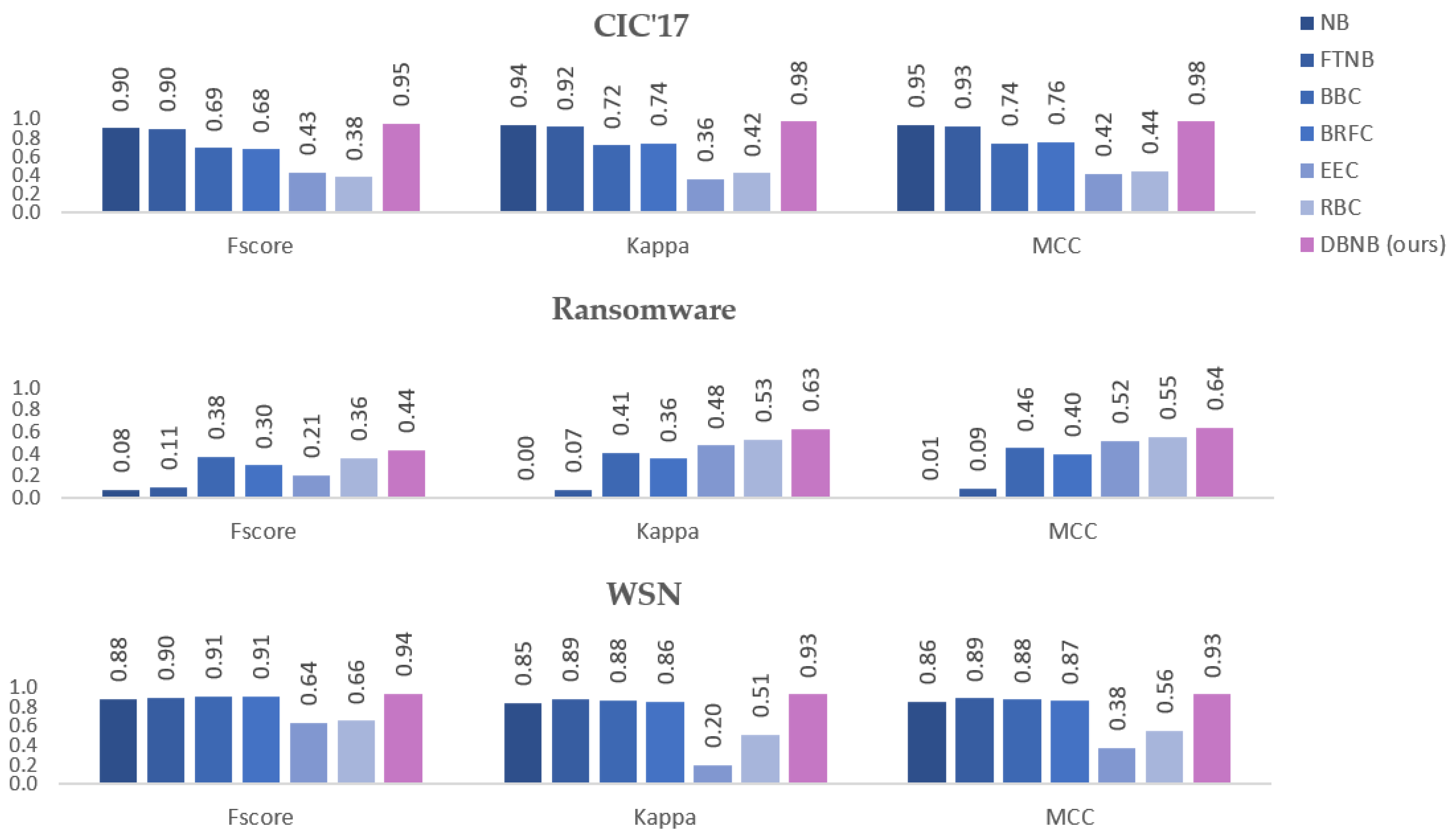
Figure 1 shows the F-score, Kappa, and MCC (macro) averages of the 10-folds cross validation. The results clearly show that CHNB consistently outperforms NB and improved FTNB with respect to all performance metrics and all three datasets. The results show that our proposed CHNB significantly outperforms all other classifiers by at least 6%, 5%, and 3% on Ransomware, CIC’17, and WSN datasets, respectively. More importantly, the results reveal that our proposed method CHNB has a very good generalization capability as it has the top performance in all three datasets and the other classifiers do not have the same consistent performance. For example, the ransomware dataset is a binary features dataset that works well with ensemble methods since one hot encoding is highly recommended for ensemble methods. In this dataset, CHNB significantly outperformed all classifiers and improved the F-score by an average of 36% compared with NB and 33% compared with FTNB. Compared with imbalanced ensemble models, CHNB significantly outperformed by 6%, 14%, 23%, and 8% for BBC, BRFC, EEC, and RBC, respectively. Similarly, our proposed method has the same consistent performance improvement for kappa and MCC scores and for the three datasets.

In the next experiment, we applied 11 different resampling methods to evaluate the performances in terms of F-score for each method combined with original NB, modified FTNB, ensemble methods, and our proposed CHNB classifiers. We used the imbalanced-learn Python package [51] to implement resampling methods with their default hyper-parameters. For efficiency, we conducted our experiments using 10% stratified sampling of WSN and Ransomware, and 1% of CIC’17 datasets. In addition, we preserved each class distribution and increased minor classes that have less than 10 examples to be at least 10 examples in the Ransomware and CIC’17 datasets. This simple modification would enable us to conduct the 10-fold experiments more reliably and to implement resampling methods that employ the kNN algorithm, which requires the minimum of four examples (neighbors) for each class.

To make a fair comparison between the classifiers, in advance, we generated 10 stratified sampling files to be used for 10-fold cross validation for each classifier and for each resampling method and we employed a paired tow-tailed t-test with the p = 0.05 significance level.

Table 5. Macro F-score for the classifiers combined with different resampling methods on the CIC’17 dataset.

Method	# Inst.	CHNB	NB	FTNB	BBC	BRC	EEC	RBC
RANDOMOS [51]	6825	99.8 ± 0.1	99.1 ± 0.2 ●	99.6 ± 0.1	99.6 ± 0.1	99.7 ± 0.1	15 ± 0.4 ●	12.3 ± 0.8 ●
SMOTE [5]	6825	99.3 ± 0.1	97.3 ± 0.2 ●	99.5 ± 0.1	99.6 ± 0.1 ○	99.7 ± 0.1 ○	13.8 ± 0.4 ●	12 ± 0.7 ●
ENN [6]	871	94.6 ± 1.5	92.3 ± 1.3	95.8 ± 1.3	72.7 ± 1.6 ●	72.9 ± 2.1 ●	41.5 ± 1.2 ●	40.7 ± 2.8 ●
TOMEKLINKS [51]	1,074	92.1 ± 1.5	81.4 ± 2 ●	92.6 ± 1.8	73 ± 1.5 ●	74.7 ± 1.1 ●	16.7 ± 0.9 ●	27.9 ± 3.9 ●
ALLKNN [51]	930	95.1 ± 1.5	90.5 ± 1.6 ●	95.8 ± 1.5	69.4 ± 2.2 ●	68.1 ± 2.9 ●	42.8 ± 1.7 ●	38.4 ± 4.5 ●
OOS [51]	667	73.6 ± 4.7	61.9 ± 4.1 ●	79.7 ± 5.3	41.5 ± 3.9 ●	37.5 ± 2.5 ●	20 ± 1.4 ●	32.7 ± 2.3 ●
SMOTEENN [7]	6524	99.5 ± 0.1	97.8 ± 0.2 ●	99.5 ± 0.1	99.8 ± 0.1	99.9 ± 0 ○	12.1 ± 0.1 ●	12 ± 0.1 ●
SMOTETOMEK [51]	6783	99.4 ± 0.1	97.3 ± 0.1 ●	99.6 ± 0.1	99.6 ± 0.1	99.8 ± 0 ○	13.8 ± 0.4 ●	10.1 ± 0.7 ●
W/T/L			0/1/7	0/8/0	1/3/4	3/1/4	0/0/8	0/0/8

,

Table 6. Macro F-score for the classifiers combined with different resampling methods on the Ransomware dataset.

Method	# Inst.	CHNB	NB	FTNB	BBC	BRC	EEC	RBC
RANDOMOS [51]	2340	95.3 ± 0.4	60.9 ± 1.1 ●	23.4 ± 1.1 ●	94.8 ± 0.6	94.4 ± 0.6	20 ± 0.7 ●	20 ± 0.8 ●
SMOTE [5]	2340	81.6 ± 1.2	57.2 ± 0.8 ●	15 ± 1.4 ●	79.4 ± 1.4	80 ± 1.4	20.9 ± 0.5 ●	22.9 ± 0.4 ●
ADASYN [58]	2335	80.4 ± 0.7	52.3 ± 0.7 ●	17.6 ± 1 ●	80.5 ± 1.3	81 ± 0.9	17 ± 0.8 ●	18 ± 1 ●
ENN [6]	335	77.9 ± 2.1	5.8 ± 0.1 ●	23.6 ± 3.1 ●	74.6 ± 4.2	76.4 ± 3.2	57.4 ± 3.2 ●	30 ± 5.7 ●
TOMEKLINKS [51]	739	46.2 ± 1.3	12.1 ± 0.5 ●	17.7 ± 0.9 ●	54 ± 1.8 ○	52 ± 1.9 ○	28.9 ± 2.7 ●	19.9 ± 1.5 ●
ALLKNN [51]	407	62.9 ± 2.2	9.5 ± 0.7 ●	48.1 ± 2.4 ●	70.5 ± 2.2 ○	85.1 ± 2.5 ○	57.7 ± 2.8 ●	31 ± 5.7 ●
OOS [51]	493	37.2 ± 0.7	7.2 ± 0.5 ●	18 ± 1.8 ●	19.6 ± 4.4 ●	19.2 ±3.6 ●	15.7 ± 2.2 ●	13.4 ± 1.8 ●
SMOTEENN [7]	1658	97.3 ± 0.9	47.9 ± 1 ●	32 ± 1.1 ●	91.6 ± 0.7 ●	97.8 ± 0.3	45.9 ± 1.6 ●	41.8 ± 2.7 ●
SMOTETOMEK [51]	2320	84.5 ± 0.7	60.2 ± 0.8 ●	13.3 ± 1.5 ●	77.7 ± 1.5 ●	81.5 ± 1.3 ●	23 ± 0.4 ●	23 ± 1.1 ●
W/T/L			0/0/9	0/0/9	2/4/3	2/5/2	0/0/9	0/9/9

and

Table 7. Macro F-score for the classifiers combined with different resampling methods on the WSN dataset.

Method	# Inst.	CHNB	NB	FTNB	BBC	BRC	EEC	RBC
RANDOMOS [51]	170,035	100 ± 0	97.4 ± 0.1 ●	100 ± 0	99.9 ± 0	100 ± 0	65.1 ± 2 ●	65.1 ± 2 ●
SMOTE [5]	170,035	99.4 ± 0	97.8 ± 0 ●	98.9 ± 0.6 ●	99.7 ± 0.6	99.8 ± 0.7	78 ± 3.9 ●	78 ± 3.9 ●
ADASYN [58]	169,967	99.4 ± 0	97.7 ± 0 ●	98.7 ± 0.1 ●	99.4 ± 0.1	99.6 ± 0.4	76.4 ± 2.1 ●	73.9 ± 2.8 ●
ENN [6]	34,471	99.3 ± 0.2	84.6 ± 0.5 ●	98.7 ± 0.2 ●	93.6 ± 0.5 ●	94.2 ± 0.3 ●	73.4 ± 2.3 ●	79.1 ± 2.2 ●
TOMEKLINKS [51]	37,078	96 ± 0.4	88.4 ± 0.4 ●	94.4 ± 0.3 ●	92.7 ± 0.3 ●	92.9 ± 0.3 ●	79.4 ± 2.7 ●	77.7 ± 3.1 ●
ALLKNN [51]	35,445	98.4 ± 0.2	85 ± 0.5 ●	97.4 ± 0.3 ●	92.8 ± 0.4 ●	94.2 ± 0.2 ●	89 ± 1.4 ●	84.7 ± 2 ●
OOS [51]	35,699	96 ± 0.4	88.4 ± 0.6 ●	94.5 ± 0.4 ●	92.6 ± 0.2 ●	92.5 ± 0.3 ●	68.3 ± 2.4 ●	70.3 ± 2.1 ●
SMOTEENN [7]	164,019	99.3 ± 0	98.4 ± 0 ●	98.9 ± 0.1 ●	99.5 ± 0.3	99.4 ± 0.4	78.1 ± 1.6 ●	83.5 ± 2.2 ●
SMOTETOMEK [51]	169,449	99.4 ± 0	97.9 ± 0 ●	98.7 ± 0 ●	99.8 ± 0.6	99.7 ± 0.4	85.6 ± 2.6 ●	76 ± 2 ●
W/T/L			0/0/9	0/1/8	0/5/4	0/5/4	0/0/9	0/0/9

show the performance on the three datasets and the significant Win/Tie/Lose (W/T/L) values are summarized at the bottom of the table. Each entry’s W/T/L in the table implies that the competitor wins on W datasets, ties on T datasets, and loses on L datasets compared with the proposed method. The field marked with ● and ○ implies that the classification performance of CHNB has statistically significant upgrades or degrades, respectively, compared with the competitor algorithm.

The results demonstrate the consistent superiority of the proposed CHNB method where it is still outperforming significantly on the averages of all datasets, except for one dataset (CIC’17), where modified FTNB has a tight result with CHNB. In terms of the best resampling technique, over-sampling alone or combined with cleaning-sampling methods substantially improves the performance of all classifiers compared with cleaning-sampling and under-sampling techniques. This is because of the many rare classes in the datasets, and since we are working with scarce data, we opted not to report two under-sampling techniques’ results.

Table 5 shows the results for the CIC’17 dataset with each classifier combined with different resampling methods. The results vary based on the resampling methods but all classifiers except for two (EEC and RBC) achieved a better performance with each resampling method compared with the base file. Among all classifiers, our proposed method CHNB and FTNB achieved the best results with no significant differences between the 10-fold F-score averages. For BBC and BRC classifiers, our proposed method CHNB significantly outperformed on four datasets compared with each classifier while BRC significantly outperformed on three datasets and BBC on only one dataset.

However, despite the minimum 10 examples per class rule that we enforced on the base file for sampling, ADASYN [58] failed to work on the CIC’17 dataset due to the kNN algorithm that could not identify enough neighbors to the major class, since we have randomly sampled the major class in the base file for efficiency, while preserving its prevalence in the dataset as a major class. This is another limitation to the diversity and the overlap drawbacks of the synthetic sample generation of SMOTE and its variants, such as ADASYN [58], whereas our method does not have any of these limitations.

For the Ransomware and WSN datasets, the results in Table 6 and Table 7 also confirm our hypothesis in regard to the robustness against the overfitting and underfitting problems that many models have. The results show that CHNB is consistently a top performer on all the resampling methods and significantly outperforms other classifiers. Despite that our method has significant improvements compared with all other classifiers, with the few exceptions of tight results sometimes with one of the ensembles’ methods or FTNB, our proposed method has a very low variance in terms of the 10-fold variations or between the different resampling methods. Moreover, in all three datasets, our proposed method is ranked among the top two classifiers. Moreover, our proposed method has a very low variance in terms of the 10-fold variations or between the different resampling methods. The results reveal that CHNB has low bias as well when the model performed better on average than other models. In fact, algorithms with few parameters, such as NB, usually have a low variance (consistency) but higher bias (low accuracy), but our proposed method generalizes well in terms of variance and bias tradeoff.

5. Discussion

The tradeoff between variance and bias is well known and models that have a lower one have a higher number for the other. Training data that are under-sampled or non-representative lead to incomplete information about the concept to predict, which causes underfitting or overfitting problems based on the model’s complexity. Models with few parameters, such as NB, will underfit the data, while ensemble models with a large number of estimates and parameters will overfit. The false discriminative attributes (noise or redundant attribute value) or the true hidden discriminative attributes (scarce data) are the cause of overfitting and underfitting scenarios. In this paper, we defined three scenarios to identify and differentiate between false and true hidden discriminate attributes. The complement harmonic average as an objective function for boosting optimization shows remarkable results to improve the base NB model. To illustrate this discrimination and to validate our claim, we will show the attributes’ hidden discrimination as the predictive power before and after the fine-tuning process of our proposed methods.

In Figure 2, we show the number of discriminative attributes as a probability heatmap for NB and CHNB. The green color indicates high discrimination, orange for moderate, and red for low discrimination, compared between attribute values within each classifier. The data used to generate the results are a binary-class (Normal vs. Attack) version of the WSN dataset and it has 17 continuous attributes with 5-bin discretization. Figure 2A is the absolute difference of the probability terms of the two classes for each attribute value, while Figure 2B shows the same difference adjusted based on the attribute value’s prevalence in the data. Figure 2 illustrates the substantial number of increased true hidden attribute values (converting to greenish color). This transformation process is symmetric since we have the sum of probability terms for attributes and for each class equal to one (

Table 8. The probability terms for the binary-class dataset before and after fine-tuning.

Attribute	Class	NB					CHNB
		val 1	val 2	val 3	val 4	val 5	val 1	val 2	val 3	val 4	val 5
Att 1	Normal	0.53	0.25	0.11	0.06	0.05	0.46	0.34	0.10	0.07	0.03
	Attack	0.32	0.22	0.21	0.12	0.13	0.07	0.04	0.06	0.03	0.79
Att 2	Normal	0.97	0.03				0.83	0.17
	Attack	0.08	0.92				0.09	0.91
Att 3	Normal	0.95	0.03	0.01	0.01	0.01	0.62	0.21	0.08	0.07	0.03
	Attack	0.99	0.01	0.00	0.00	0.00	1.00	0.00	0.00	0.00	0.00
Att 4	Normal	0.83	0.16	0.01	0.00	0.00	0.64	0.31	0.04	0.01	0.00
	Attack	0.98	0.02	0.00	0.00	0.00	0.97	0.03	0.00	0.00	0.00
Att 5	Normal	1.00					1.00
	Attack	1.00					1.00
Att 6	Normal	0.95	0.05				0.70	0.30
	Attack	1.00	0.00				1.00	0.00
Att 7	Normal	0.14	0.86				0.21	0.79
	Attack	0.92	0.08				0.91	0.09
Att 8	Normal	1.00	0.00	0.00	0.00		0.95	0.04	0.01	0.00
	Attack	0.76	0.19	0.05	0.00		0.17	0.67	0.16	0.00
Att 9	Normal	1.00	0.00	0.00	0.00		1.00	0.00	0.00	0.00
	Attack	0.67	0.24	0.05	0.03		0.16	0.63	0.14	0.07
Att 10	Normal	0.18	0.82				0.24	0.76
	Attack	0.92	0.08				0.91	0.09
Att 11	Normal	0.82	0.12	0.04	0.01	0.01	0.62	0.25	0.09	0.03	0.01
	Attack	0.97	0.02	0.01	0.00	0.00	0.95	0.03	0.02	0.01	0.00
Att 12	Normal	0.60	0.29	0.07	0.02	0.01	0.58	0.23	0.14	0.03	0.02
	Attack	0.98	0.02	0.00	0.00	0.00	0.97	0.02	0.00	0.00	0.00
Att 13	Normal	0.91	0.04	0.02	0.02	0.01	0.45	0.22	0.12	0.14	0.06
	Attack	0.97	0.00	0.01	0.01	0.00	0.99	0.00	0.00	0.00	0.00
Att 14	Normal	0.98	0.01	0.00	0.00	0.00	0.83	0.08	0.03	0.02	0.04
	Attack	0.87	0.03	0.02	0.01	0.06	0.19	0.01	0.02	0.01	0.77
Att 15	Normal	0.84	0.01	0.05	0.07	0.02	0.24	0.03	0.27	0.34	0.12
	Attack	0.85	0.01	0.06	0.07	0.01	0.98	0.00	0.01	0.01	0.00
Att 16	Normal	0.55	0.34	0.09	0.02	0.01	0.66	0.20	0.10	0.02	0.02
	Attack	0.97	0.02	0.00	0.00	0.00	0.96	0.03	0.00	0.00	0.00
Att 17	Normal	1.00					1.00
	Attack	1.00					1.00

). Therefore, any attribute value converting to green is, by design, making the complement attribute value convert from green to red (the opposite). This will increase the hidden true discriminative attribute values and decrease the false ones that are considered as noise and redundancy during the fine-tuning process.

The consistent performance gain compared with other classifiers on diverse datasets and the magnitude of difference compared with NB indicates the capability of CHNB to capture complex relations to closely fit the training data. The results in Section 4.1 and Section 4.2 show that boosting the model on a scant dataset needs to be carefully implemented to balance the tradeoff between bias and variance. The deterioration of the model to balance the tradeoff is instigated by the boosting algorithm complexity when it terminates and not continuing to improve the base model on unseen data. We can clearly see this in the imbalanced datasets where ensemble models (EEC and RBC), which are boosting algorithms, failed to generalize well on unseen data compared with bagging algorithms (BBC and BRF). The FTNB boosting algorithm terminates earlier than CHNB on average, which has more iterations toward harmonizing the probability terms and balancing the data. However, more iteration means more training time, and CHNB is slower compared with FTNB, and has tight results compared with the ensembles’ methods. In

Table 9. Average number of iterations for fine-tuning methods and execution time for the classifiers.

Dataset		Iterations #		Execution Time in Minutes
		CHNB	FTNB	CHNB	FTNB	NB	BBC	BRC	EEC	RBC
CIC-IDS 2017 [55]		22.3	8.8	6.8	5.2	1.6	2.1	4.0	9.7	8.1
Ransomware [56]		18.7	4.5	5.3	4.2	1.1	3.8	3.9	14.2	6.8
WSN [57]		12.4	7.1	4.3	2.9	0.5	2.0	8.7	6.3	4.9
UIC 41 datasets [50]	Min	4	4	2.1	1.7	0.5
	Avg	9.4	8.6				-	-	-	-
	Max	21.7	22.5

, we report the running time for each method and the number of epochs of the fine-tuning process for CHNB compared with FTNB. All of the experiments were conducted on a machine with a 3.2 GHz Apple M1 Pro chip with 10 CPU cores and 32 GB of RAM.

In Table 9, we can see that FTNB terminates the fine-tuning process earlier than CHNB as clearly seen in the Ransomware dataset with the fewest iterations and the most outperformed results. On the other hand, bagging ensemble methods (BBC and BRC) are faster than boosting methods (EEC and RBC) due to the parallel implementation capability of bagging algorithms. In addition, since we are updating the probability terms during the fine-tuning process, the inference time of the proposed CHNB and the FTNB are similar to the original NB classifier’s time.

6. Conclusions

This work proposed a discriminative fine-tuning algorithm to alleviate the scant or imbalanced datasets’ effects on estimating reliable probability terms of the Naïve Bayes classifier. The proposed algorithm (CHNB) determines the size of the update amount (weights) for each attribute value based on the complement classes’ harmonic average (predicted vs actual class) of the probability terms. This makes the update size large when rare and common classes have very skewed or scarce data and are small otherwise. We evaluated the performance of the proposed algorithm with respect to F-score, kappa, and MCC metrics on imbalanced benchmark datasets, as well as the accuracy on general datasets. Our empirical analysis revealed that, with respect to the F-score, CHNB significantly outperforms NB (36%, 6%, and 5%) and FTNB (33%, 4%, and 5%) on three imbalanced benchmark datasets. Compared with imbalanced ensemble methods, CHNB significantly outperforms by at least 6%, 3%, and 26% on the same benchmark datasets. In addition, we tested the effects of the proposed method on 41 UCI general benchmark datasets, and the results also showed improvements by at least 1.38% on average, with respect to accuracy, compared with NB, FTNB, and five state-of-art attribute weighting NB. As a suggestion for future work, we intend to investigate using the proposed method on a Bayesian network classifier and to develop a gradient-based objective function.