Configuration Optimization and Response Prediction Method of the Clamping Robot for Vibration Suppression of Cantilever Workpiece

Abstract

Cantilever workpieces are widely used in the aerospace field; they produce vibrations easily and affect machining quality under the action of external forces. Enhancing the stiffness of the workpiece using a robot as a fixture is an effective means to solve this problem. However, the vibration suppression effect of the clamping system depends on the dynamics performance of different configurations of the robot. Therefore, in order to obtain the optimal clamping robot configuration, the system dynamics model composed of automated guided vehicle (AGV)-robot-gripper-workpiece (ARGW) is established based on the transfer matrix method of the multibody system (MSTMM), and the vibration responses of the workpiece under different configurations are analyzed. Then, a robot configuration optimization method based on workpiece response was proposed. Finally, the effectiveness of the optimization method is verified through simulations and experiments at different clamping robot configurations. The dynamics model and optimization method in this paper can be used to predict the workpiece vibration response and choose a reasonable clamping robot configuration, avoiding the reduction in workpiece machining quality due to the improper configuration of the clamping robot.

1. Introduction

Cantilever workpieces on aerospace products have characteristics that include a complex structure, poor stiffness, and high precision requirements, and often require special fixtures to reduce their machining vibration [1]. Moreover, the diversity of cantilever workpiece types poses a high challenge to the selection of fixtures. Industrial robots have been widely used in the manufacturing of aerospace products with low costs, high mobility and strong adaptability [2,3,4,5], and have gradually become an important choice for fixed large-size structure and cantilever workpieces. For example, the cantilever workpieces on the space station have poor stiffness, making it easy to produce vibration under the action of external forces and thus affecting the machining quality. Enhancing the stiffness through the mobile clamping robot can effectively suppress the vibration, and avoid the disadvantages of traditional processes such as repeated assembly, which entails a complex process, and long cycle. However, the operation performance of the robot will change with the configuration [6,7,8], resulting in the unstable vibration suppression effect of different clamping robot configuration on the workpiece, and cannot meet the requirements of machining quality [9,10]. Consequently, optimizing the configuration of the clamping robot is very important to improve the machining quality of the clamped workpiece.

Extensive studies on robot configuration optimization based on kinematics [11,12,13], stiffness [14,15,16], and dynamic performance [17,18] have been carried out to date. Generally, the robot configuration optimization based on kinematic performance is mainly used to ensure the track smoothness and task accessibility of large-range machining such as milling and welding [13,19,20]. However, in order to improve the machining quality of the workpiece, the robot stiffness is necessary to be considered in the configuration optimization [21,22]. When the external excitation frequency is not close to the natural frequency of the robot system, the configuration optimization effect based on static stiffness is enough [15,23]. For example, Sebastien [24] and Guo et al. [25] built a robot static stiffness model based on the robot six-joint stiffness and Jacobian matrix, and guaranteed the drilling quality of the robot by analyzing and optimizing the stiffness at different configurations. Actually, there are six stiffness parameters on each joint of the robot. Accordingly, in order to accurately analyze the stiffness performance of the robot under different configurations, Cui et al. [26] established a dynamic model including 36 stiffness parameters based on the transfer matrix method of the multibody system (MSTMM). In addition, for processing tasks such as drilling and milling, the machining quality is mainly affected by the stiffness in the axial direction and the feed direction [27]. Bu [14] and Chen et al. [28] ensured the optimal stiffness in the direction of the main machining load by using the robot orientation stiffness optimization model, and the experimental results proved that the optimization method could effectively improve the machining quality. The above methods are based on the redundant degree-of-freedom (DOF) of the six-joint robot when performing five DOF tasks. However, due to the fixed position relationship between the robot and the workpiece, the improvement effect of the configuration optimization is limited. Hence, Caro et al. [29] first analyzed the optimal configuration in the working space according to the robot stiffness model, and then ensured that the robot is in the ideal configuration by adjusting the fixed position of the workpiece. Similarly, Shen et al. [30] improved the stiffness performance of the robot by optimizing the fixed angle between the flange and the spindle, which ensured the quality of the robot drilling. Zhang et al. [31] investigated an initial position optimization method for the welding robot based on the digital twin model, which found the initial welding position with the best operational smoothness through a particle swarm algorithm to ensure the welding efficiency. Although the above methods have significant effects on the machining of small parts, the optimization effects are limited for large-size parts machining, and may even prevent the configuration optimization of the robot due to operating range limitations [32,33]. On these grounds, a robot system with mobile platform is gradually adopted to manufacture large structural parts. Jiao et al. [11] used the additional axis of the robot to divide the position of the wing drilling, and optimized the robot configuration based on the static stiffness model, which effectively ensured the operation stiffness of the robot in the whole task. Moreover, when the automated guided vehicle (AGV) is used as the robot fixed platform, the flexibility of the robot system can be further improved, which ensures that the robot has redundant DOF to performing the task [34]. Nevertheless, due to the poor stiffness of AGV, its influence on the stiffness performance of the robot system should be considered when performing the configuration optimization, and the complex structure greatly increases the difficulty of stiffness modelling.

The machining vibration of the robot depends on its dynamic performance. Due to the weak stiffness and asymmetric structure of the robot, it is more prone to chatter (self-excited vibration), which is one of the biggest obstacles in the pursuit of machining quality [35,36]. In order to prevent the chatter during milling, Chen et al. [18] adopted the stable lobe diagram under different robot configurations established by the inverse distance weighted model for configuration optimization. Likewise, Said [17] and He et al. [37] analyzed the machining vibration and optimized the whole milling trajectory based on the robot dynamics model, realizing the avoidance of machining chatter with non-process parameters adjustment. When no chatter occurs, the vibration response of the workpiece should be reduced as much as possible to further improve the surface machining quality. Li et al. [38] took the spindle vibration response as the index and combined it with genetic algorithm to optimize the robot configuration, and reduced the vibration response by changing the configuration to realize the improvement of the drilling quality. Considering the above studies, it can be seen that the robot configuration optimization based on the dynamics performance can directly reduce the vibration response and improve the machining quality. However, the existing studies are mainly aimed at the vibration suppression of the robot machining system with the open-loop structure, and the clamping robot has not been sufficiently investigated. In addition, when the robot acts as a fixture to fix the cantilever workpiece on aerospace products, the workpiece forms an approximately closed-loop structure with the clamping robot system, which increases the difficulty of analyzing the dynamics performance and selecting the appropriate robot configuration.

Inspired by the above mentioned studies, this paper combines dynamics response prediction and configuration optimization to improve the vibration suppression effect for the cantilever workpiece. In order to enable the clamping robot to suppress the vibration of the workpiece at different positions on the space station, the AGV is used as the carrier. The established dynamics model of the AGV-robot-gripper-workpiece (ARGW) system can predict the vibration response of the workpiece in the clamped state. Then, the influence of different configurations of the clamping robot caused by different clamping directions, different workpieces, and movement of the AGV on the vibration response of the workpiece were analyzed. The simulation and experimental results show that the proposed configuration optimization method of the clamping robot can not only improve the vibration suppression effect, but also avoid the degradation of machining quality caused by improper configuration. The main contributions of this method can be summarized as follows:

• Providing a solution for dynamics modelling of the ARGW system with approximately closed-loop structure;
• The influence laws of different clamping robot configurations on the vibration responses of the workpiece are studied;
• The vibration suppression effect on the workpiece is improved by optimizing the clamping robot configuration.

The rest of this paper is organized as follows. The dynamics model and its topology structure of the ARGW system are given in Section 2. In Section 3, the solution method of dynamics responses under different configurations of the clamping robot is deduced according to the MSTMM. In Section 4, the influence laws of different configurations on vibration responses are analyzed, and the configuration optimization method based on the workpiece responses is shown. In Section 5, the vibration suppression effect of the configuration optimization is verified using simulations and experiments. Finally, the conclusions are presented in Section 6.

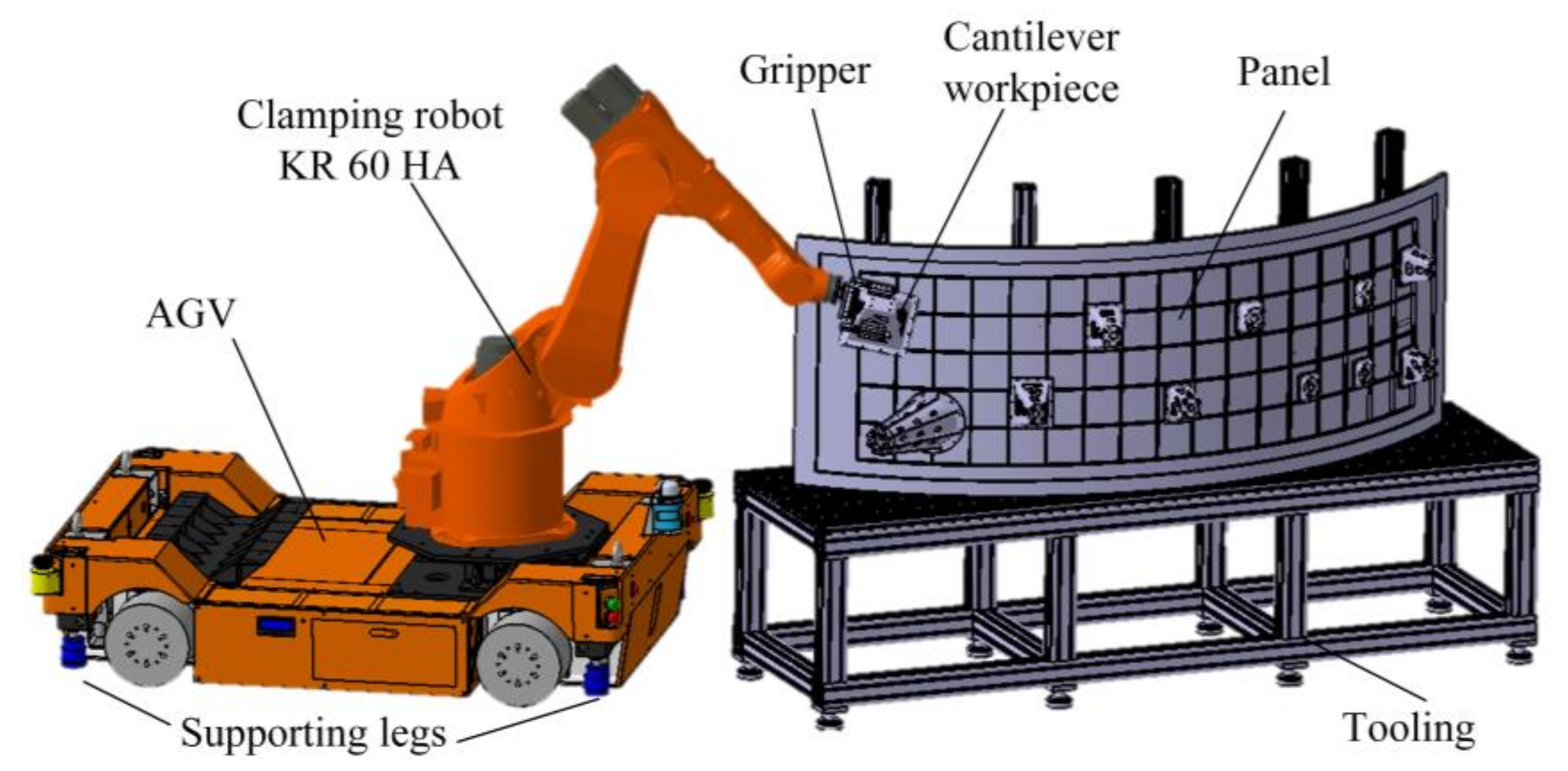
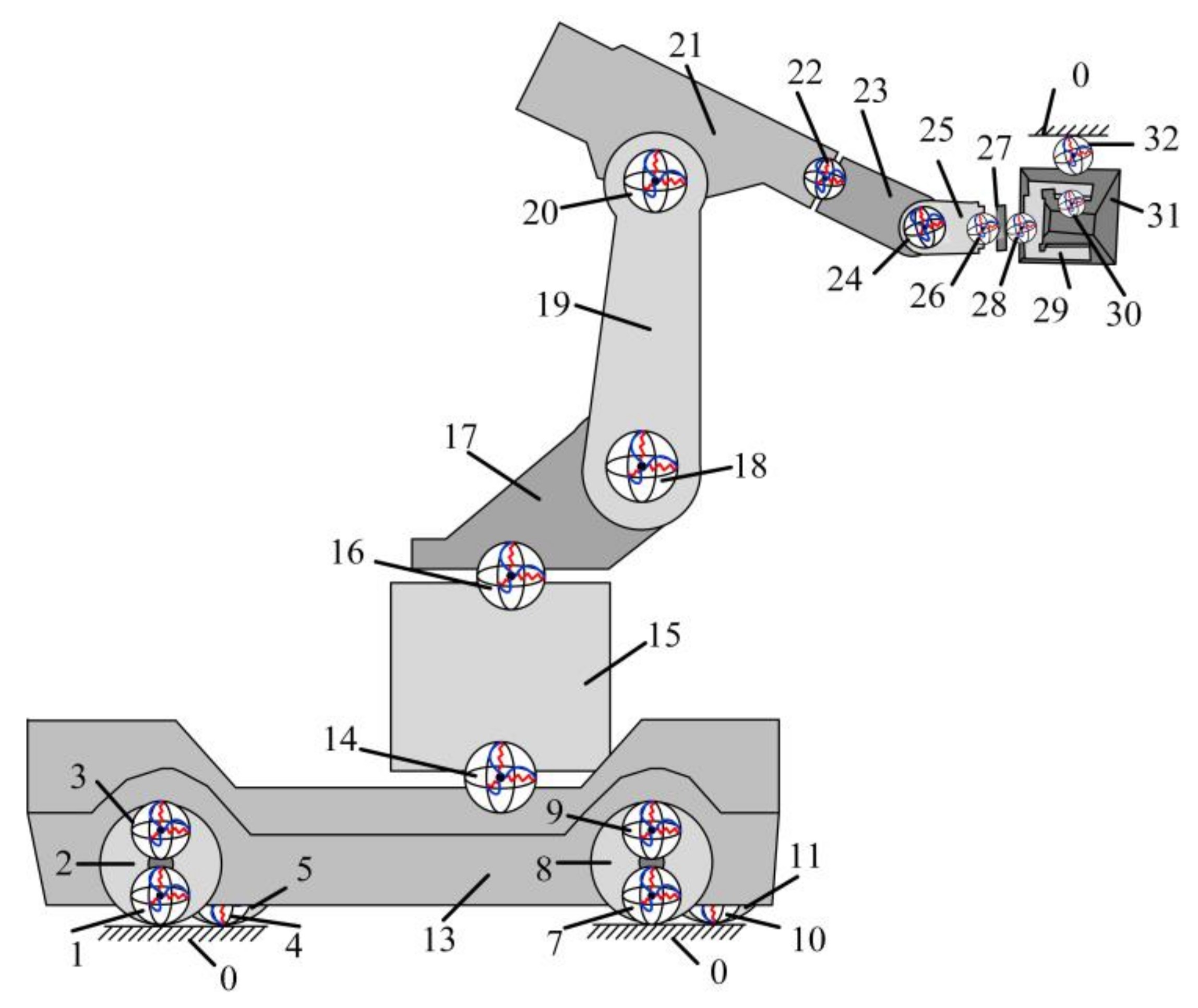
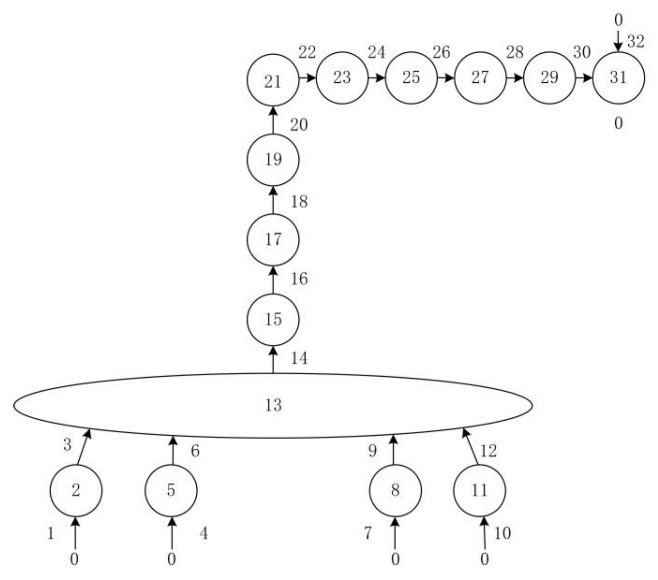
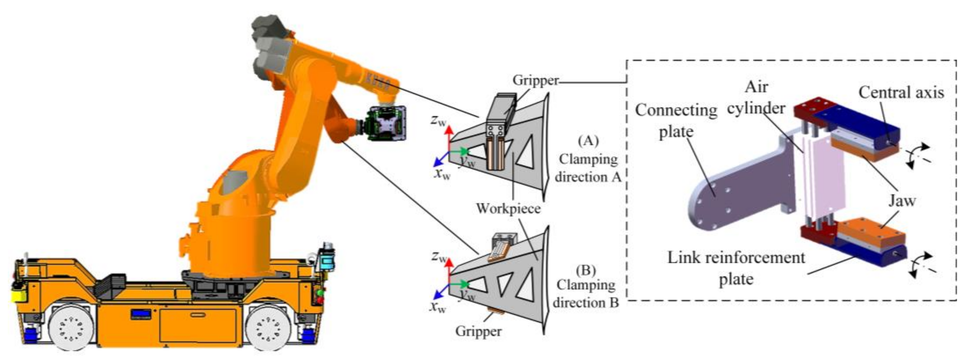
2. System Composition and Dynamic Model

As shown in Figure 1, the large panel is a component sample of the space station cabin. Due to the good stiffness of the panel and tooling, they are considered a fixed boundary in this paper. When the AGV is well-positioned, the supporting legs will extend and support the AGV to improve the stability of the system. At this time, both the supporting legs of the AGV and the cantilever workpiece are in contact with the fixed boundaries, resulting in an approximate closed-loop structure of the ARGW system composed of AGV, clamping robot KR 60 HA, gripper, and cantilever workpiece.

The elements in the ARGW system can be divided into rigid body elements and hinge elements. Moreover, rigid body elements include single input end and single output end elements, multiple input ends and single output end elements. Synchronously, hinge elements are unified as spatial elastic hinge elements with three-direction translational stiffness and three-direction rotational stiffness.

The dynamics model of the system is described in Figure 2, and its topology figure is shown in Figure 3. The four supporting legs, AGV, seven links of the robot, gripper, and workpiece are considered rigid bodies 2, 5, 8, 11, 13, 15, 17, 19, 21, 23, 25, 27, 29, and 31, respectively. Additionally, the hinge elements are numbered as 1, 3, 4, 6, 7, 9, 10, 12, 14, 16, 18, 20, 22, 24, 26, 28, 30, and 32 in sequence. The ground and the panel are fixed boundaries, all of which are numbered as 0. In addition, the workpiece machining surface is a free boundary, also numbered 0.

It can be seen that the topology figure of the system dynamics model is a tree structure, where the output end 0 of the workpiece 31 is the tip of the system and the elements 1, 4, 7, 10, and 32 are the roots of the system. Arrows and rectangles are divided into hinge elements and body elements, and the beginning and end of arrows coincide with the output end of the previous body element and the input end of the next body element, respectively. Furthermore, the direction of the arrow is the transfer direction of the state vector Z in the ARGW system.

3. Dynamics Responses of the Workpiece under Different Clamping Robot Configurations

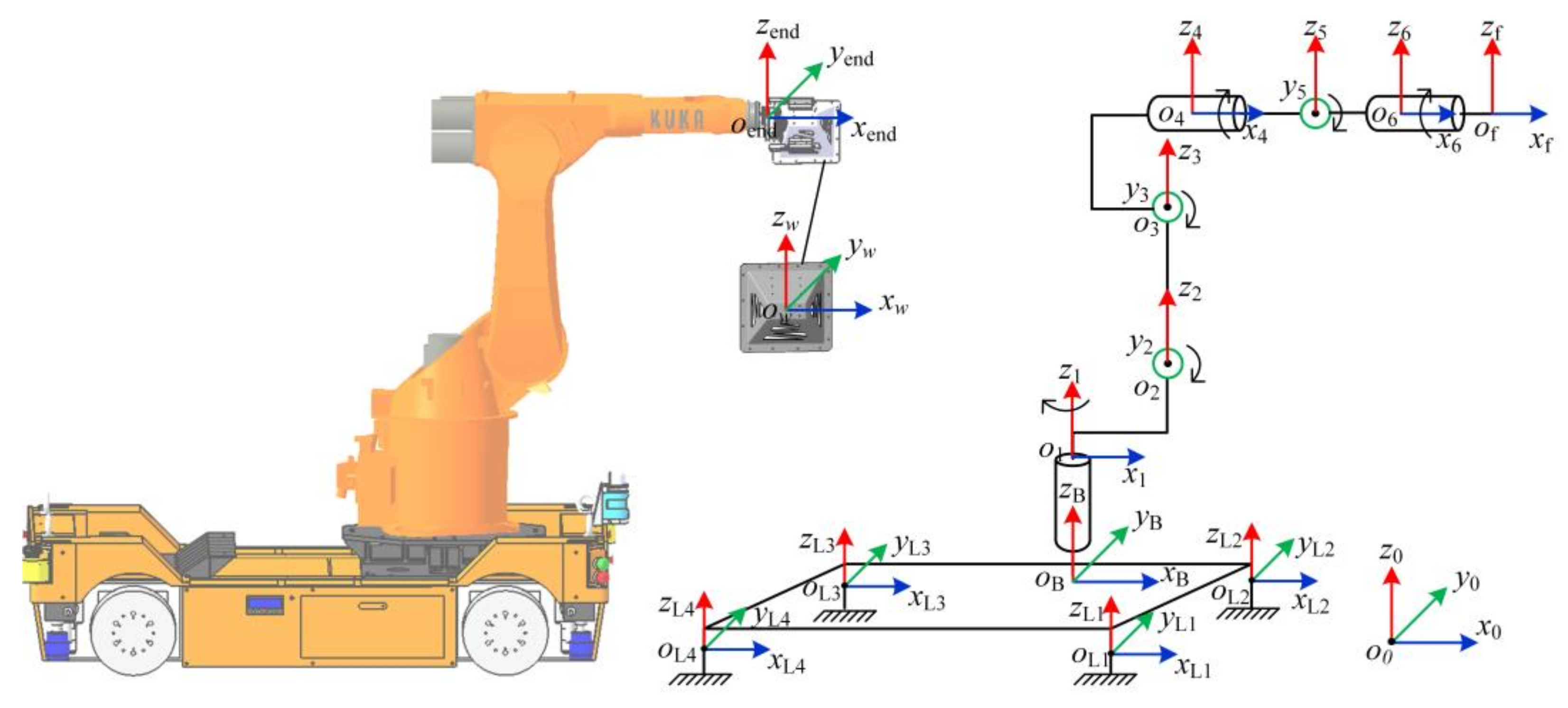
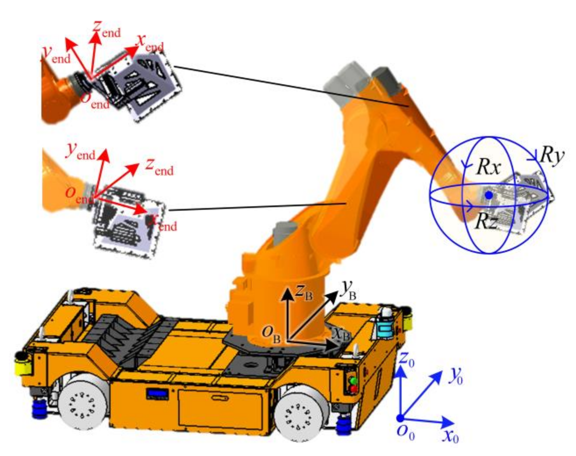
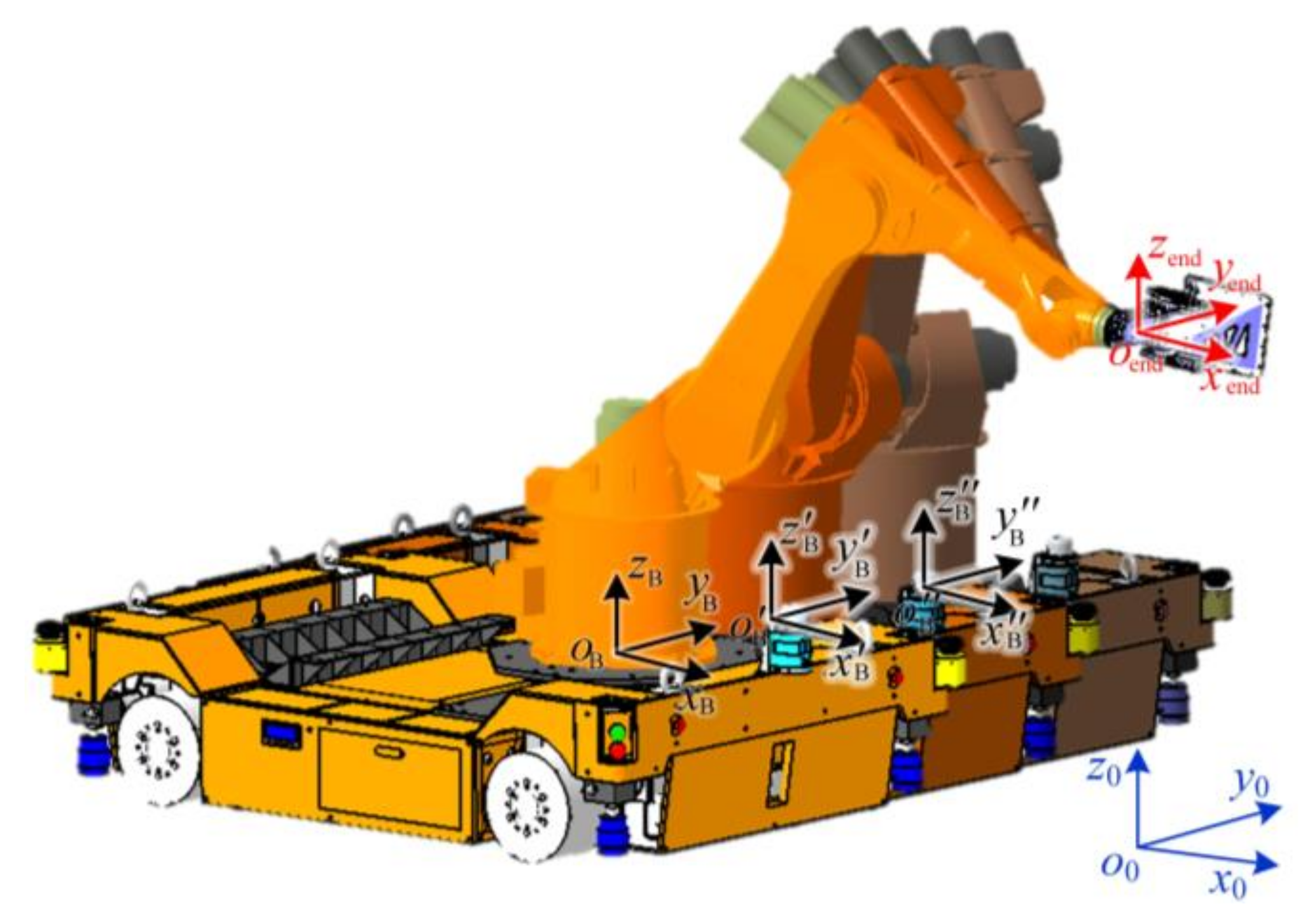
3.1. Coordinate Systems of the ARGW System

The diagrams of the body element and the hinge element are shown in Figure 4a and b, respectively, which are located in the same world coordinate system o₀x₀y₀z₀. In particular, the mass of the body element is C, its dynamics parameters are measured by the model, and the coordinate system of the input end Ix′y′z′ and the coordinate system of the output end Oxyz are always in same direction. Moreover, the translational stiffness and torsional stiffness of the hinge element are identified using the mode test, and the coordinate system of the input end and output end coincide. Furthermore, defining the coordinate system Oxyz of the body element and the coordinate system Ix′y′z′ of the next hinge element always coincide; thus, the coordinate system of the ARGW system can be represented by the Oxyz of the body element.

As shown in Figure 5, $o_{\mathrm{L}i}{x}_{\mathrm{L}i}{y}_{\mathrm{L}i}{z}_{\mathrm{L}i}(i=1,\hspace{0.17em}2,\hspace{0.17em}3,\hspace{0.17em}4)$ are the coordinate systems of four supporting legs, $o_{\mathrm{L}i}{x}_{\mathrm{L}i}{y}_{\mathrm{L}i}{z}_{\mathrm{L}i}\hspace{0.33em}(i=1,\hspace{0.17em}2,\hspace{0.17em}3,\hspace{0.17em}4)$ is the coordinate system of the AGV, $o_i{x}_i{y}_i{z}_i\hspace{0.17em}(i=1,\hspace{0.17em}2,\hspace{0.17em}\cdots ,\hspace{0.17em}6,\hspace{0.17em}\mathrm{f}\hspace{0.17em})$ are the six-link and flange coordinate systems of the robot, o_endx_endy_endz_end and o_wx_wy_wz_w are the end gripper and workpiece coordinate systems, respectively.

When the clamping robot is in the configuration shown in Figure 5, all coordinate systems have the same direction, and the angles of the six joints of the robot are defined as 0°. After the robot’s configuration changes, the transfer direction of the state vector of each joint will change. Depending on the different rotation directions of six joints, the transformation matrices of x, y, and z directions are defined as follows:

$$H_x\left({\theta }_k\right)=\left[\begin{array}{cccc}{h}_x\left({\theta }_k\right)& O_{3\times 3}& O_{3\times 3}& O_{3\times 3}\\ O_{3\times 3}& h_x\left({\theta }_k\right)& O_{3\times 3}& O_{3\times 3}\\ O_{3\times 3}& O_{3\times 3}& h_x\left({\theta }_k\right)& O_{3\times 3}\\ O_{3\times 3}& O_{3\times 3}& O_{3\times 3}& h_x\left({\theta }_k\right)\end{array}\right],\hspace{0.33em}\hspace{0.33em}k=1,\hspace{0.17em}2,\hspace{0.17em}3,4,5,6$$

(1)

$$H_y\left({\theta }_k\right)=\left[\begin{array}{cccc}{h}_y\left({\theta }_k\right)& O_{3\times 3}& O_{3\times 3}& O_{3\times 3}\\ O_{3\times 3}& h_y\left({\theta }_k\right)& O_{3\times 3}& O_{3\times 3}\\ O_{3\times 3}& O_{3\times 3}& h_y\left({\theta }_k\right)& O_{3\times 3}\\ O_{3\times 3}& O_{3\times 3}& O_{3\times 3}& h_y\left({\theta }_k\right)\end{array}\right],\hspace{0.33em}\hspace{0.33em}k=1,\hspace{0.17em}2,\hspace{0.17em}3,4,5,6$$

(2)

$$H_z\left({\theta }_k\right)=\left[\begin{array}{cccc}{h}_z\left({\theta }_k\right)& O_{3\times 3}& O_{3\times 3}& O_{3\times 3}\\ O_{3\times 3}& h_z\left({\theta }_k\right)& O_{3\times 3}& O_{3\times 3}\\ O_{3\times 3}& O_{3\times 3}& h_z\left({\theta }_k\right)& O_{3\times 3}\\ O_{3\times 3}& O_{3\times 3}& O_{3\times 3}& h_z\left({\theta }_k\right)\end{array}\right],\hspace{0.33em}\hspace{0.33em}k=1,\hspace{0.17em}2,\hspace{0.17em}3,4,5,6$$

(3)

where ${\theta }_k$ is the angle of the joint k.

$$h_x(\theta )=\left[\begin{array}{ccc}1& 0& 0\\ 0& \cos \theta & \sin \theta \\ 0& -\sin \theta & \cos \theta \end{array}\right],h_y(\theta )=\left[\begin{array}{ccc}\cos \theta & 0& -\sin \theta \\ 0& 1& 0\\ \sin \theta & 0& \cos \theta \end{array}\right],h_z(\theta )=\left[\begin{array}{ccc}\cos \theta & \sin \theta & 0\\ -\sin \theta & \cos \theta & 0\\ 0& 0& 1\end{array}\right]$$

(4)

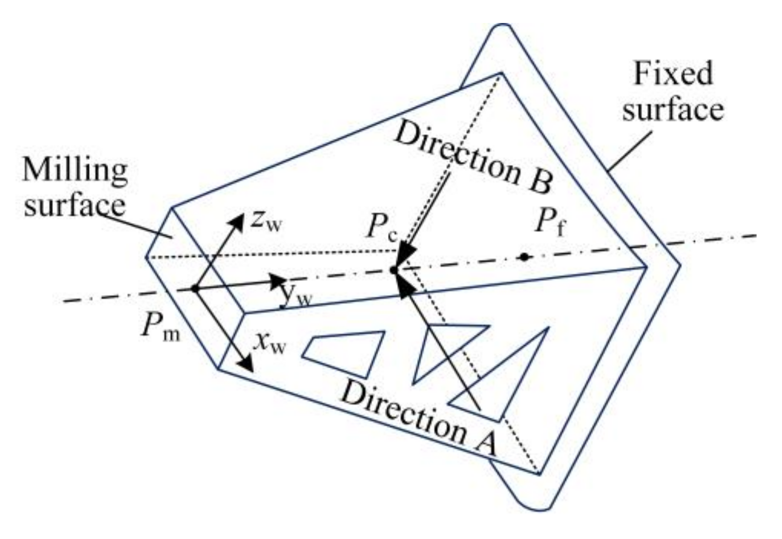
3.2. Dynamics Response of the Workpiece

In MSTMM [39], the state vector Z used to represent the motion state of the object is defined as follows:

$$Z={[\begin{array}{cccccccccccc}X& Y& Z& {\mathrm{\Theta }}_x& {\mathrm{\Theta }}_y& {\mathrm{\Theta }}_z& M_x& M_y& M_z& Q_x& Q_y& Q_z\end{array}]}^{\mathrm{T}}$$

(5)

where ${\left[X,\hspace{0.17em}\hspace{0.33em}Y,\hspace{0.33em}Z\right]}^{\mathrm{T}}$, ${\left[{\mathrm{\Theta }}_x,\hspace{0.33em}{\mathrm{\Theta }}_y,\hspace{0.33em}{\mathrm{\Theta }}_z\right]}^{\mathrm{T}}$, ${\left[M_x,\hspace{0.33em}{M}_y,\hspace{0.33em}{M}_z\right]}^{\mathrm{T}}$, and ${\left[Q_x,\hspace{0.33em}{Q}_y,\hspace{0.33em}{Q}_z\right]}^{\mathrm{T}}$ are linear displacements, angular displacements, internal torques, and internal forces relative to its equilibrium position in modal coordinates, respectively [40,41].

According to the dynamics model and the automatic deduction, the main transfer equation of the ARGW system is established as follows:

$$T_{31-32}{Z}_{32,0}+T_{31-1}{Z}_{1,0}+T_{31-4}{Z}_{4,0}+T_{31-7}{Z}_{7,0}+T_{31-10}{Z}_{10,0}=Z_{31,0}$$

(6)

where $Z_{k,0}$ are the reprintings of the state vector of the output end of element k, and

$$\left\{\begin{array}{c}{\mathit{T}}_{31-32}={\mathit{U}}_{31,32}{\mathit{U}}_{32}\hfill \\ {\mathit{T}}_{31-1}={\mathit{U}}_{31,30}{\mathit{U}}_{30}{\mathit{U}}_{29}{\mathit{U}}_{28}{\mathit{U}}_{27}{\mathit{H}}_X\left({\theta }_6\right){\mathit{U}}_{26}{\mathit{U}}_{25}{\mathit{H}}_Y\left({\theta }_5\right){\mathit{U}}_{24}{\mathit{U}}_{23}{\mathit{H}}_X\left({\theta }_4\right){\mathit{U}}_{22}{\mathit{U}}_{21}{\mathit{H}}_Y\left({\theta }_3\right)\hfill \\ \hspace{1em}{\mathit{U}}_{20}{\mathit{U}}_{19}{\mathit{H}}_Y\left({\theta }_2\right){\mathit{U}}_{18}{\mathit{U}}_{17}{\mathit{H}}_Z\left({\theta }_1\right){\mathit{U}}_{16}{\mathit{U}}_{15}{\mathit{U}}_{14}{\mathit{U}}_{13,3}{\mathit{U}}_3{\mathit{U}}_2{\mathit{U}}_1\hfill \\ {\mathit{T}}_{31-4}={\mathit{U}}_{31,30}{\mathit{U}}_{30}{\mathit{U}}_{29}{\mathit{U}}_{28}{\mathit{U}}_{27}{\mathit{H}}_X\left({\theta }_6\right){\mathit{U}}_{26}{\mathit{U}}_{25}{\mathit{H}}_Y\left({\theta }_5\right){\mathit{U}}_{24}{\mathit{U}}_{23}{\mathit{H}}_X\left({\theta }_4\right){\mathit{U}}_{22}{\mathit{U}}_{21}{\mathit{H}}_Y\left({\theta }_3\right)\hfill \\ \hspace{1em}{\mathit{U}}_{20}{\mathit{U}}_{19}{\mathit{H}}_Y\left({\theta }_2\right){\mathit{U}}_{18}{\mathit{U}}_{17}{\mathit{H}}_Z\left({\theta }_1\right){\mathit{U}}_{16}{\mathit{U}}_{15}{\mathit{U}}_{14}{\mathit{U}}_{13,6}{\mathit{U}}_6{\mathit{U}}_5{\mathit{U}}_4\hfill \\ {\mathit{T}}_{31-7}={\mathit{U}}_{31,30}{\mathit{U}}_{30}{\mathit{U}}_{29}{\mathit{U}}_{28}{\mathit{U}}_{27}{\mathit{H}}_X\left({\theta }_6\right){\mathit{U}}_{26}{\mathit{U}}_{25}{\mathit{H}}_Y\left({\theta }_5\right){\mathit{U}}_{24}{\mathit{U}}_{23}{\mathit{H}}_X\left({\theta }_4\right){\mathit{U}}_{22}{\mathit{U}}_{21}{\mathit{H}}_Y\left({\theta }_3\right)\hfill \\ \hspace{1em}{\mathit{U}}_{20}{\mathit{U}}_{19}{\mathit{H}}_Y\left({\theta }_2\right){\mathit{U}}_{18}{\mathit{U}}_{17}{\mathit{H}}_Z\left({\theta }_1\right){\mathit{U}}_{16}{\mathit{U}}_{15}{\mathit{U}}_{14}{\mathit{U}}_{13,9}{\mathit{U}}_9{\mathit{U}}_8{\mathit{U}}_7\hfill \\ {\mathit{T}}_{31-10}={\mathit{U}}_{31,30}{\mathit{U}}_{30}{\mathit{U}}_{29}{\mathit{U}}_{28}{\mathit{U}}_{27}{\mathit{H}}_X\left({\theta }_6\right){\mathit{U}}_{26}{\mathit{U}}_{25}{\mathit{H}}_Y\left({\theta }_5\right){\mathit{U}}_{24}{\mathit{U}}_{23}{\mathit{H}}_X\left({\theta }_4\right){\mathit{U}}_{22}{\mathit{U}}_{21}{\mathit{H}}_Y\left({\theta }_3\right)\hfill \\ \hspace{1em}{\mathit{U}}_{20}{\mathit{U}}_{19}{\mathit{H}}_Y\left({\theta }_2\right){\mathit{U}}_{18}{\mathit{U}}_{17}{\mathit{H}}_Z\left({\theta }_1\right){\mathit{U}}_{16}{\mathit{U}}_{15}{\mathit{U}}_{14}{\mathit{U}}_{13,12}{\mathit{U}}_{12}{\mathit{U}}_{11}{\mathit{U}}_{10}\hfill \end{array}\right.$$

(7)

where $U_i$ is the transfer matrix corresponding to the element i, $U_{31,30}$ and $U_{31,32}$ are the transfer matrices of workpiece with respect to input ends 30 and 32, $U_{13,3}$, $U_{13,6}$, $U_{13,9}$, and $U_{13,12}$ are the transfer matrices of the AGV with respect to input ends 3, 6, 9, and 12.

From the topology figure of the ARGW system, it can be seen that the workpiece and the AGV are multiple input ends and single output end. Therefore, the geometric equation of the workpiece can be obtained as follows:

$$G_{31-32}{Z}_{32,0}+G_{31-1}{Z}_{1,0}+G_{31-4}{Z}_{4,0}+G_{31-7}{Z}_{7,0}+G_{31-10}{Z}_{10,0}=0_{6\times 1}$$

(8)

where

$$\begin{array}{l}{G}_{31-1}=H_{31,\hspace{0.33em}30}{U}_{31,30}^{-1}{T}_{31-1}\\ G_{31-4}=H_{31,\hspace{0.33em}30}{U}_{31,30}^{-1}{T}_{31-4}\\ G_{31-7}=H_{31,\hspace{0.33em}30}{U}_{31,30}^{-1}{T}_{31-7}\\ G_{31-10}=H_{31,\hspace{0.33em}30}{U}_{31,30}^{-1}{T}_{31-10}\\ G_{31-32}=-H_{31,\hspace{0.33em}32}{U}_{32}\end{array}$$

(9)

Furthermore, the geometric equations of the AGV are

$$\begin{array}{l}{G}_{13-1}{Z}_{1,0}+G_{13-4}{Z}_{4,0}=0_{6\times 1}\\ G_{13-1}{Z}_{1,0}+G_{13-7}{Z}_{7,0}=0_{6\times 1}\\ G_{13-1}{Z}_{1,0}+G_{13-10}{Z}_{10,0}=0_{6\times 1}\end{array}$$

(10)

where

$$\begin{array}{l}{G}_{13-1}=-H_{13,\hspace{0.33em}3}{U}_3{U}_2{U}_1\\ G_{13-4}=H_{13,\hspace{0.33em}6}{U}_6{U}_5{U}_4\\ G_{13-7}=H_{13,\hspace{0.33em}9}{U}_9{U}_8{U}_7\\ G_{13-10}=H_{13,\hspace{0.33em}12}{U}_{12}{U}_{11}{U}_{10}\end{array}$$

(11)

The specific form of coefficient matrix $H_{i,o}$ is

$$H_{i,o}=\left[\begin{array}{cccc}{I}_3& {\tilde{l}}_{io}& O_{3\times 3}& O_{3\times 3}\\ O_{3\times 3}& I_3& O_{3\times 3}& O_{3\times 3}\end{array}\right],\hspace{0.33em}\hspace{0.33em}\left\{\begin{array}{l}i=13\\ o=3,6,9,12\end{array}\right.\hspace{0.33em}or\hspace{0.33em}\left\{\begin{array}{l}i=31\\ o=30,32\end{array}\right.$$

(12)

where $l_{io}$ represents the displacement matrix of the output point end o relative to first input end i, ${\tilde{l}}_{io}$ refers to the skew-symmetric matrix of $l_{io}$.

Equations (8) and (10) are the geometric equations of the ARGW system. By combining the geometric equations with Equation (6), the overall transfer matrix can be written as follows:

$$\left[\begin{array}{cccccc}-{\mathit{I}}_{12}& {\mathit{T}}_{31-32}& {\mathit{T}}_{31-1}& {\mathit{T}}_{31-4}& {\mathit{T}}_{31-7}& {\mathit{T}}_{31-10}\\ {\mathit{O}}_{6\times 12}& {\mathit{G}}_{31-32}& {\mathit{G}}_{31-1}& {\mathit{G}}_{31-4}& {\mathit{G}}_{31-7}& {\mathit{G}}_{31-10}\\ {\mathit{O}}_{6\times 12}& {\mathit{O}}_{6\times 12}& {\mathit{G}}_{13-1}& {\mathit{G}}_{13-4}& {\mathit{O}}_{6\times 12}& {\mathit{O}}_{6\times 12}\\ {\mathit{O}}_{6\times 12}& {\mathit{O}}_{6\times 12}& {\mathit{G}}_{13-1}& {\mathit{O}}_{6\times 12}& {\mathit{G}}_{13-7}& {\mathit{O}}_{6\times 12}\\ {\mathit{O}}_{6\times 12}& {\mathit{O}}_{6\times 12}& {\mathit{G}}_{13-1}& {\mathit{O}}_{6\times 12}& {\mathit{O}}_{6\times 12}& {\mathit{G}}_{13-10}\end{array}\right]\left[\begin{array}{c}{\mathit{Z}}_{31,0}\\ {\mathit{Z}}_{32,0}\\ {\mathit{Z}}_{1,0}\\ {\mathit{Z}}_{4,0}\\ \begin{array}{c}{\mathit{Z}}_{7,0}\hfill \\ {\mathit{Z}}_{10,0}\hfill \end{array}\end{array}\right]=0$$

(13)

It can be simplified as follows:

$$U_{\mathrm{all}}{Z}_{\mathrm{all}}=0_{72\times 1}$$

(14)

By removing the 0 element and its corresponding array in the boundary conditions, Equation (14) is further simplified as follows:

$${\overline{U}}_{\mathrm{all}}{\overline{Z}}_{\mathrm{all}}=0$$

(15)

Then, the eigenfrequency equation of the ARGW system can be written as follows:

$$\det {\overline{U}}_{\mathrm{all}}=0$$

(16)

Solving Equation (16), the natural frequency ${\omega }^k(k=1,2,3\cdots 6)$ of the ARGW system can be obtained. Then, the state vector of the workpiece can be solved by taking ${\omega }^k$ into Equation (13). However, to analyze the vibration suppression effect of the ARGW system, it is necessary to convert the state vector to the physical coordinate system based on the dynamics model.

The dynamics equation of rigid body element i is as follows:

$$M_i{v}_{i,tt}+C_i{v}_{i,t}+K_i{v}_i=f_i$$

(17)

where $M_i$, $C_i$ and $K_i$ are the mass matrix, damping matrix, and stiffness matrix of the rigid body i. Additionally, $v_i$ is the displacement generated by the external forces $f_i$, and $v_{i,t}$, $v_{i,tt}$ are the first and second derivatives of $v_i$ with respect to time t. By superimposing the dynamics equation of each rigid body element according to the topology structure of the ARGW system, the overall dynamics equation can be written as follows:

$$M{v}_{tt}+C{v}_t+Kv=f$$

(18)

According to the MSTMM, Equation (18) can be expressed as follows:

$${\ddot{q}}^k(t)+2{\zeta }^k{\omega }^k{\dot{q}}^k(t)+{({\omega }^k)}^2{q}^k(t)={\displaystyle {\sum }_i\left(〈f(t),V_i^k〉/M_i^k\right)}$$

(19)

where ${\ddot{q}}^k$, ${\dot{q}}^k$, and $q^k$ are the generalized acceleration, velocity, and displacement, respectively. The eigenvector $V_i^k$ contains only the liner displacement and angular displacement of the state vector $Z_i^k$. Then, the dynamics responses v can be obtained as follows:

$$v={\displaystyle \sum _{k=1}^n{V}^k{q}^k(t)}$$

(20)

The machining vibration responses of the workpiece can be obtained by bringing the milling forces into Equation (19). Further, the change laws of clamping robot’s vibration suppression on the workpiece with different configurations can be analyzed.

4. Dynamics Simulation and Configuration Optimization Method

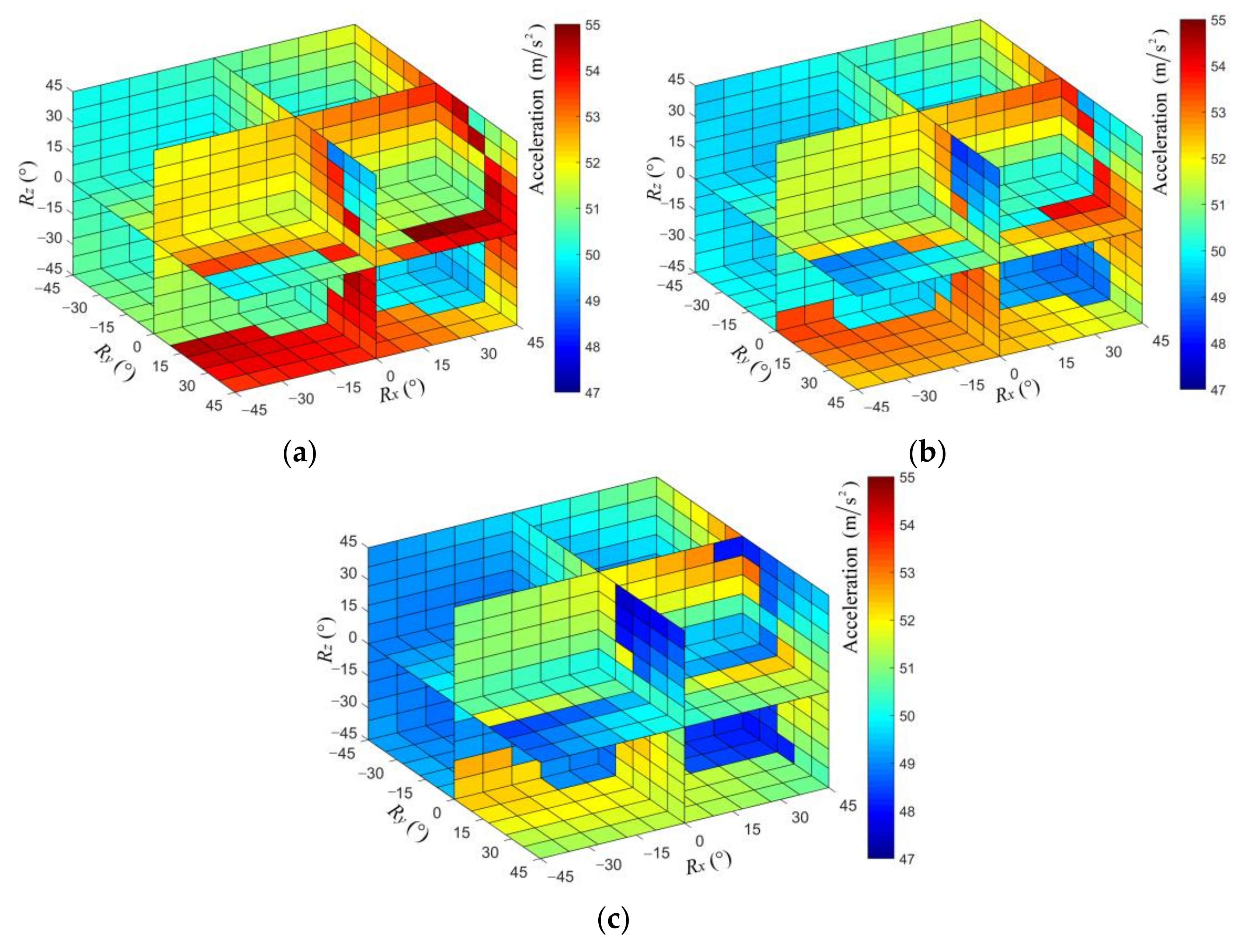
4.1. Vibration Suppression Effects of Different Postures

The configuration of the clamping robot can be divided into two parts: the position x_endy_endz_end and posture RxRyRz of the flange coordinate system relative to the coordinate system $o_B{x}_B{y}_B{z}_B$. Additionally, the values of the position and posture will both affect the configuration of the clamping robot.

As shown in Figure 6, the gripper consists of a connecting plate, an air cylinder, two link reinforcement plates, two jaws and two central axes, in which the jaws can adjust around the central axis. Before clamping, the gripper is left open. When the configuration of the clamping robot is determined, the cylinder contracts to clamp the workpiece, and the jaws adaptively adjust the angles to fit the surfaces of the workpiece. The clamping force of the gripper on the workpiece is only related to the air pressure and cylinder performance, and will not change with the clamping position and clamping direction. When the spatial positions of the AGV and workpiece remain unchanged, the gripper can still clamp the workpiece through both the A and B directions. Apparently, the clamping robot has different configurations in the two directions of the gripper.

The vibration responses of the workpiece depend on the state vector Z_31,0 of the output point P_m, which can be written as follows:

$$Z_{31,0}=U_{31,30}{Z}_{30,31}+U_{31,32}{Z}_{32,31}$$

(21)

As shown in Figure 7, when the gripper is clamping the workpiece in direction A or B, the input points of two directions are equivalent to P_c. Additionally, P_c is located on the line over the output point P_m and the input point P_f, and its position is constant relative to P_m in both directions, A and B. Moreover, the dynamics parameters of the workpiece are unchanged; thus, the transfer matrix $U_{31,30}$ is also unchanged. Furthermore, since the fixed position of the workpiece is always unique, then the transfer matrix $U_{31,32}$ is also unchanged. In this case, the vibration responses of the workpiece are only related to $Z_{30,31}$ and $Z_{32,31}$ at different clamping robot configurations. In this paper, the acceleration of the P_m point in the o_wx_wy_wz_w coordinate system is used to represent the vibration response of the workpiece.

In addition to different RxRyRz for the same workpiece, the configurations of the clamping robot facing the same type of workpiece with different fixed angles on the panel will also change. As shown in Figure 8, when the gripper clamping the workpiece in the B direction, the configuration of the clamping robot is constantly changing with the fixed angle of the workpiece. At this time, if the position of the AGV and the fixed stiffness of the workpiece do not change, only RxRyRz changes in the robot configuration. The same is true for clamping direction A. For the two cases in Figure 6 and Figure 8, the influence of different RxRyRz on the vibration suppression effect of the clamping robot needs to be analyzed to obtain the optimal clamping configuration.

In order to analyze and predict the vibration suppression effect of different clamping robot configurations on the workpiece, the dynamic milling force model of spiral slotting end mill is used as the input, and the instantaneous milling force in x_w, y_w, and z_w direction is as follows:

$$\left\{\begin{array}{l}{F}_x={\displaystyle \sum _{j=1}^N{\displaystyle \sum _{l=1}^M(-\mathrm{d}{F}_{\mathrm{t}jl}\cos {\varphi }_{jl}-\mathrm{d}{F}_{\mathrm{r}jl}\sin {\varphi }_{jl})}}\\ F_y={\displaystyle \sum _{j=1}^N{\displaystyle \sum _{l=1}^M(-\mathrm{d}{F}_{\mathrm{r}jl}\cos {\varphi }_{jl}+\mathrm{d}{F}_{\mathrm{t}jl}\sin {\varphi }_{jl})}}\\ F_z={\displaystyle \sum _{j=1}^N{\displaystyle \sum _{l=1}^M\mathrm{d}{F}_{ajl}}}\end{array}\right.$$

(22)

where jl represents the lth cutting microelement on the cutting blade j, ${\varphi }_{jl}$ is the angular displacement of the microelement, while dF_tjl, dF_rjl, and dF_ajl are the forces on the feed, normal, and axial direction, respectively.

The milling parameters in

Table 1. Milling parameters.

Feed Rate (mm/s)	Rotational Speed (r/min)	Milling Width (mm)	Milling Depth (mm)
2.5	6000	8.0	1.0

are adopted to simulate the vibration suppression effects of different RxRyRz at three heights, and the variation laws of the overall workpiece responses are shown in Figure 9a–c, respectively. where $x_{\mathrm{end}}=1.8\hspace{0.33em}\mathrm{m}$, $y_{\mathrm{end}}=0\hspace{0.33em}\mathrm{m}$, and $z_{\mathrm{end}}=1.0\hspace{0.17em}\mathrm{m},\hspace{0.33em}1.2\hspace{0.17em}\mathrm{m},\hspace{0.33em}1.4\hspace{0.17em}\mathrm{m}$.

The three axes in Figure 9 represent the angles of Rx, Ry, and Rz, and the color represents the amplitudes of the responses, which are determined by the acceleration response legend on the right side of the figure. Each figure is composed of six faces, of which the middle three groups of intersecting faces are the responses of different configurations when Rx = 0°, Ry = 0°, and Rz = 0°, and the three faces at the edge are the responses when Rx = 45°, Ry = −45°, and Rz = −45°. From the face corresponding to Ry = 0° in Figure 9a, it can be seen that as Rz gradually changes from −45° to 45°, the responses tend to gradually increase, indicating that the vibration suppression effect of the clamping robot is gradually reduced. In addition, it can be seen from the face of Rx = 45° and Rz = −45° that when Ry > 0°, the responses are greater than Ry < 0°. Moreover, Figure 9b,c presents the same pattern of response changes.

As can be seen from the simulation results of different heights, the overall responses of the workpiece show a downward trend as the height increases from 1.0 m to 1.4 m. Additionally, the maximum values of the overall responses at the three heights are approximately 55 m/s², 54 m/s², and 53 m/s², respectively. The maximum change range of responses throughout the simulation interval is 7 m/s². Furthermore, the change ranges caused by Rx and Rz are significantly smaller than that of Ry. This is because the conversion around Rx is mainly completed by the robot’s fourth and sixth joints, which will not produce a large configuration change. Moreover, the RxRyRz of the robot are almost symmetrical when rotating around the positive and negative directions of Rz, and the differences of vibration suppression effect of the corresponding RxRyRz are minor. In contrast, the configuration change around Ry is large and asymmetric, and responses also change greatly. It can be seen from Figure 9 that when Ry is greater than 0, the responses are significantly greater, which indicates that the vibration suppression effect corresponding to the clamping direction B in Figure 7 is better than the clamping direction A.

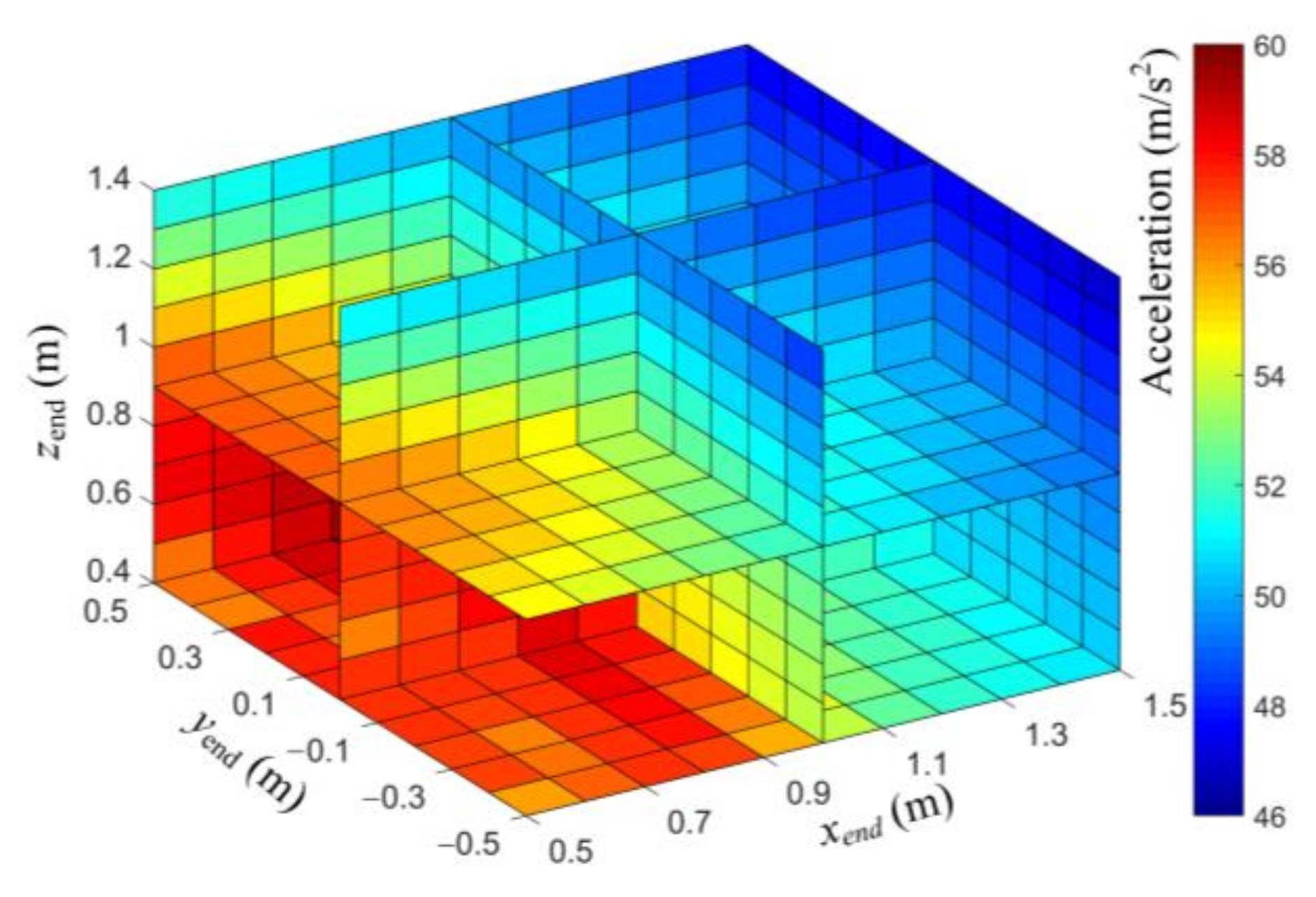
4.2. Vibration Suppression Effects of Different Positions

As indicated in Figure 10, the movement of the AGV in the x₀o₀y₀ allows the robot to clamp the same workpiece in different configurations. In addition to the movement along the direction of y₀ in Figure 10, it can also move along the direction of x₀, which provides great freedom for the choice of the clamping robot configuration. Although the positions of the coordinate system o₀x₀y₀z₀ and o_endx_endy_endz_end are constant, the x_end and y_end of the clamping robot changes. Moreover, the height of the end z_end changes when facing the workpiece at different positions in space. Therefore, it is necessary to comprehensively analyze the vibration suppression effect of different x_endy_endz_end.

Similarly, based on the conditions in Section 4.1, a simulation is conducted to analyze the influence of the configuration changes caused by x_endy_endz_end on vibration responses, and the results are depicted in Figure 11.

Similar to the presentation in Figure 9, the three axes are x_end, y_end, and z_end, and the figure is composed of six faces too. However, the difference is that the vibrational response caused by the x_endy_endz_end changes more regularly. The overall response showed a decreasing trend from the boundary of x = 0.5 m and z = 0.4 m to the boundary of x = 1.5 m and z = 1.4 m. It can be intuitively seen from Figure 11 that as the configuration of clamping robot changes, the overall responses of the workpiece vary from 46 m/s² to 60 m/s², and the change range reaches 14 m/s². Compared with RxRyRz, the change in x_endy_endz_end has a more obvious effect on the vibration suppression of the clamping robot. In addition, the responses of the workpiece decrease with the increase in z_end, which is consistent with the result shown in Figure 9. Additionally, the effect of y_end change on vibration responses is not as obvious as that of x_end and z_end. This is because the robot is approximately symmetric along y_end = 0, and the configuration change caused by the of y_end is not as obvious as that of x_end and y_end. In short, the law in Figure 11 shows that the closer the workpiece is to $o_B{x}_B{y}_B{z}_B$, the worse the vibration suppression effect of the corresponding configuration of the clamping robot is.

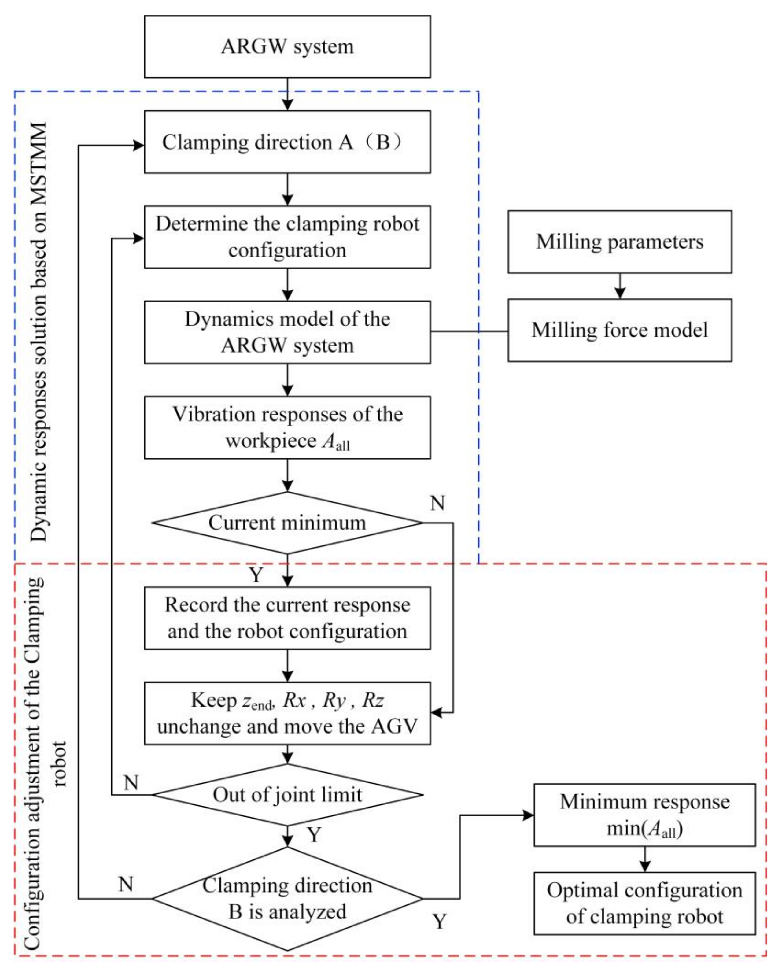
4.3. Configuration Optimization Mothed of the Clamping Robot

The configuration optimization process can be divided into two parts: dynamic responses solving and configuration adjustment, where configuration adjustment can be achieved by changing the clamping direction of the gripper and the position of the AGV. When the workpiece and its clamping direction are determined, the configuration of the clamping robot is only related to x_end and y_end. In addition, the current z′_end and R′xR′yR′z need to be kept unchanged in the optimization of the same clamping direction. Additionally, the specific process is shown in Figure 12. The blue dotted box is the dynamics modeling and response analysis, the red dotted box is the configuration optimization part, and the milling force model is the external force input of the entire optimization process. Additionally, after each configuration change, a dynamic response solution is required.

During configuration optimization, the overall response A_all of the workpiece output point P_m is taken as an index, which can be expressed as follows:

$$A_{\mathrm{all}}=\sqrt{a_x^2+a_y^2+a_z^2}$$

(23)

where a_x, a_y, and a_z are the responses in three directions of the P_m.

With reference to the technical parameters of the KR 60 HA robot, the joint limit of the clamping robot can be determined. Then, the configuration optimization model of clamping robot was established as follows:

$$\left\{\begin{array}{l}\min \left(A_{\mathrm{all}}\right)\\ s.t. \left(z_{\mathrm{end}},Rx,Ry,Rz\right)\hspace{0.33em}=\left({z^{\prime }}_{\mathrm{end}},R^{\prime }x,R^{\prime }y,R^{\prime }z\right)\hspace{0.33em}\\ {\theta }_k\in \left[{\theta }_{p\min },{\theta }_{p\max }\right],\hspace{0.33em}\hspace{0.33em}k=1,2,\cdots ,6\end{array}\right.$$

(24)

where [${\theta }_{k\min },\hspace{0.33em}{\theta }_{k\max }$] is the movable range of joint k.

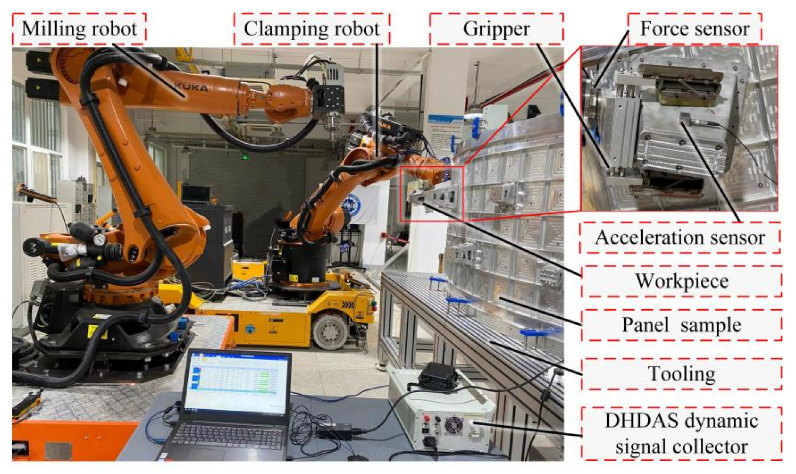
5. Verification Experiments

5.1. Verification of the ARGW System Dynamics Model

To verify the accuracy of the dynamics model and the effectiveness of the configuration optimization method, the experimental platform is built in Figure 13. The milling robot is KR 210 R2700, and the workpiece milling surface is 6061 aluminum alloy. In the middle of the clamping robot flange and gripper is a six-dimensional force sensor that can be used to collect the forces applied on the clamping robot during milling. In addition, the clamping status of the workpiece by the gripper can be monitored using the data on the force sensor. When the configuration of the clamping robot remains unchanged, the data of the force sensor after clamping is equal to the previous clamping, it means that the clamping force of the workpiece is consistent and determined by the gripper. In this way, the influence of the clamping force on the vibration suppression effect is excluded. Moreover, the responses of the workpiece are collected by the three-component acceleration sensor and DHDAS dynamic signal collector.

In the verification experiment, the [x_end, y_end, z_end, Rx, Ry, Rz] of the clamping robot were [0.78 m, 0.36 m, 1.03 m, 140.79°, 67.89°, 40.54°]. The workpiece was milled using the process parameters in Table 1, and the responses of the workpiece in the experiment were collected using the acceleration sensor. The forces information collected by the force sensor is converted into the o_wx_wy_wz_w coordinate system, and the forces are presented in Figure 14 after compensating the initial forces information and gravity. In general, the feed and radial forces are greater than the axial forces. Since the milling direction in this paper is the negative direction of z_w, the forces in x_w and z_w directions are significantly greater than those in y_w direction. By inputting the milling forces into the ARGW system dynamics model, the workpiece acceleration response can be obtained. Compared with the responses collected by the acceleration sensor, the results are shown in Figure 15.

Figure 15a–c presents the responses in the x_w, y_w, and z_w directions, respectively. From the acceleration responses in the three directions, it can be seen that the responses increase rapidly and then decrease at the beginning stage, and the responses in the middle stage tend to be stable, finally decreasing slowly at the end stage. This is because when the tool first enters the workpiece, the instantaneous excitation will make the workpiece produce a large response. As the tool moves away from the workpiece, the response decreases as the amount of cutting decreases. It can be seen from the local magnification diagram that the responses of the experiment and the simulation agree well overall. Specifically, the maximum error is 4.6 m/s², appearing in the x_w direction, whereas the average errors in the three directions are only 2.9%, 3.4%, and 2.3%. The comparative results demonstrate the accuracy of the dynamics model of the ARGW system. Moreover, the simulated responses are always smaller than the experimental responses in either direction. This is because there are various environmental noises in the experiment, while the simulation is carried out in an ideal environment without additional interfering factors.

5.2. Verification of the Configuration Optimization Method

Under the experimental conditions in Section 5.1, the x_end and y_end are changed to realize the vibration suppression with different configurations of the clamping robot. Then, the vibration suppression effects of different configurations are analyzed and predicted by the dynamics model, and the result is represented in Figure 16.

Figure 16 is the acceleration response plane when z_end = 1.03 m in Figure 11. In order to show the amplitude of the response more intuitively, a vertical coordinate named acceleration is added in this figure on the basis of retaining color features. In addition, the two axes in the horizontal plane are x_end and y_end. The responses in Figure 15 show a trend of gradually decreasing from the highest point P_max to the surrounding, and its overall change law is almost consistent with that shown in Figure 11. Under current conditions, the response is up to 67.98 m/s² of the P_max, and the response can be reduced by 45.35% to 37.15 m/s² after configuration optimization of the clamping robot. At the maximum response point P_max, the corresponding x_end of the clamping robot is only 0.5 m, and y_end is basically close to 0 m. At this time, the gripper of the robot is closest to the base as shown in Figure 16. Therefore, in order to obtain a better vibration suppression effect, the configuration of the clamping robot should be as far away from P_max as possible.

According to the simulation result, a series of experiments are carried out to verify the accuracy of the response prediction and the effectiveness of the configuration optimization method. Including a group of non-clamping experiments and four groups of clamping experiments with different configurations, the experimental scenes are shown in Figure 17. The configuration of the clamping robot in Figure 17e is the optimized configuration, while Figure 17b–d shows the controlled experiments with three groups of gradually decreasing responses.

In Figure 17, it can be observed that the angles of six joints of the milling robot are (−16.49°, −63.64°, 77.45°, 168.90°, 63.04°, −224.17°), and the slight configuration changes caused by the different milling processes are ignored. Additionally, the configurations of the four groups of the clamping robot are listed in

Table 2. Configurations of the clamping robot.

Group	${\mathit{\theta }}_1 \mathbf{(}°\mathbf{)}$	${\mathit{\theta }}_2 \mathbf{(}°\mathbf{)}$	${\mathit{\theta }}_3 \mathbf{(}°\mathbf{)}$	${\mathit{\theta }}_4 \mathbf{(}°\mathbf{)}$	${\mathit{\theta }}_5 \mathbf{(}°\mathbf{)}$	${\mathit{\theta }}_6 \mathbf{(}°\mathbf{)}$
Config. 1	56.85	−54.88	95.82	−248.27	42.74	−147.21
Config. 2	61.13	−58.51	101.86	−241.47	40.89	−152.49
Config. 3	47.09	−52.77	92.24	102.02	49.46	−142.27
Config. 4	37.73	−29.41	49.91	86.66	36.88	243.70

. Moreover, the values of x_end and y_end corresponding to Config. 1 to Config. 4 gradually move away from point P_max. The responses of the experiments and simulations are indicated in Figure 18.

As can be seen from Figure 18, the response gradually decreases as the Config. 1 runs to Config. 4, which is consistent with the change in the response prediction result observed in Figure 16. Moreover, the experimental responses are 2.55 m/s², 1.71 m/s², 2.16 m/s², and 2.01 m/s² larger than the simulated responses, respectively, which agrees with the comparison results in Figure 15. The above results also verify the accuracy of the response prediction based on the ARGW system dynamics model. The response corresponding to the optimized Config. 4 is the smallest of the four sets of configurations. The experimental result is 46.78 m/s², and the simulation result is 44.77 m/s². Furthermore, the simulated and experimental responses were reduced by 15.37 m/s² and 15.91 m/s² after configuration optimization, demonstrating the effectiveness of configuration optimization in improving the vibration suppression effect.

The milling experiment effects of different configurations are illustrated in Figure 18; in addition, the surface roughness of the corresponding milling path is listed in

Table 3. Surface roughness of the milling path.

Group	Non- Clamping	Config. 1	Config. 2	Config. 3	Config. 4
Ra (μm)	1.684	0.921	0.801	0.611	0.576

. Additionally, C1 to C4 are abbreviations of Config. 1 to Config. 4.

It can be intuitively observed from Figure 19 that the non-clamping milling surface has obvious tool marks, and its surface roughness reaches 1.684, which is significantly higher than that of the other four groups of clamping experiments. The result proves that the mobile clamping robot system is an effective solution for the vibration suppression of the cantilever workpiece. From Config. 1 to Config. 4, the experimental vibration response of the workpiece is 62.9 m/s², 59.36 m/s², 51.63 m/s², 46.78 m/s² successively, decreasing by 3.54 m/s², 7.73 m/s², 4.85 m/s², respectively. The corresponding surface roughness values were 0.921, 0.801, 0.611 and 0.576, which decreased by 0.12, 0.19 and 0.035, respectively. It can be observed that with the decrease in workpiece vibration response, surface machining quality is gradually improved because the surface roughness is not only affected by vibration, but also related to the geometry of the tool, the workpiece material, the product chipping and so on. Therefore, the amplitude of vibration response reduction cannot be directly mapped linearly to the roughness value. In addition, compared with the milling track in Config.4, burrs appeared on the edges of other tracks, which also confirmed that the occurrence of burr defects in the workpiece was affected by the response amplitude. The changes in surface roughness and burrs prove that the robot configuration optimization based on workpiece response in this paper can effectively improve the machining quality of workpiece.

6. Conclusions

This paper aims to improve the vibration suppression effect on the cantilever workpiece through configuration optimization. Due to the complex structure and poor stiffness of the robot and the AGV, as well as the approximate closed-loop structure of the ARGW systems, it is difficult to predict the vibration response. For the optimal vibration suppression, the dynamics model of the ARGW system was established based on the MSTMM considering the robot stiffness changing with configuration, and the configuration optimization was carried out with the workpiece response as the index. Through simulation analysis and experimental results, the following conclusions can be drawn.

Through simulation and experimental comparison, it is found that the response obtained from the dynamics model is approximately 1.5% to 3.4% lower than the experiment; however, the overall agreement is good. The comparison results verify the accuracy of the ARGW system dynamics model established in this paper. The influence laws of different clamping robot configurations on the response were simulated based on the dynamics model. According to the simulation results, the closer the robot end is to the base coordinate system, the worse the vibration suppression effect on the workpiece will be. When the gripper clamping the workpiece in z_end = 1.03 m, the maximum response obtained using the simulation is located at P_max point (x_end = 0.5 m, y_end = 0 m), reaching 67.98 m/s². Then, the response of the workpiece was reduced to 44.77 m/s² using the configuration optimization method. In the experiments, the workpiece’s surface roughness decreases from 0.921 to 0.576 as the response decreases from 62.69 m/s² to 46.78 m/s² after the configuration optimization of the clamping robot. Although the workpiece vibration response is not linearly related to the surface roughness, optimizing the configuration of the clamping robot based on the workpiece response can effectively improve the machining quality.

In fact, in addition to the configuration of the clamping robot, there are many factors that affect the vibration response of the workpiece. In order to further improve the vibration suppression effect of the system in the future research, influence factors such as the gripper position, clamping force, and machining parameters should be considered. In addition, it is necessary to further establish the dynamics model of the dual-robot cooperative machining system and analyze the influence of the milling robot on the machining quality of the workpiece. Furthermore, the mapping relationship between workpiece vibration response and surface roughness can be explored to provide the basis for obtaining the ideal machining quality.

References

1. Yang, Y.; Yang, Y.; Xiao, M.; Wan, M.; Zhang, W. A Gaussian process regression-based surrogate model of the varying workpiece dynamics for chatter prediction in milling of thin-walled structures. Int. J. Mech. Syst. Dyn. 2022, 2, 117–130. [Google Scholar] [CrossRef]
2. Zeng, Y.; Tian, W.; Li, D.; He, X.; Liao, W. An error-similarity-based robot positional accuracy improvement method for a robotic drilling and riveting system. Int. J. Adv. Manuf. Technol. 2016, 88, 2745–2755. [Google Scholar] [CrossRef]
3. Zhao, B.; Zeng, L.; Wu, Z.; Xu, K. A continuum manipulator for continuously variable stiffness and its stiffness control formulation. Mech. Mach. Theory 2020, 149, 103746. [Google Scholar] [CrossRef]
4. Cen, L.; Melkote, S.N. Effect of Robot Dynamics on the Machining Forces in Robotic Milling. Procedia Manuf. 2017, 10, 486–496. [Google Scholar] [CrossRef]
5. Moreira, A.P.; Neto, P.; Vidal, F. Special Issue on Advances in Industrial Robotics and Intelligent Systems. Appl. Sci. 2023, 13, 1352. [Google Scholar] [CrossRef]
6. Schneider, U.; Posada, J.R.D.; Verl, A. Automatic Pose Optimization for Robotic Processes. In Proceedings of the 2015 IEEE International Conference on Robotics and Automation (ICRA), Seattle, WA, USA, 26–30 May 2015. [Google Scholar]
7. Zhang, D.; Yuan, H.; Cao, Z. Environmental adaptive control of a snake-like robot with variable stiffness actuators. IEEE/CAA J. Autom. Sin. 2020, 7, 745–751. [Google Scholar] [CrossRef]
8. Guo, Y.; Dong, H.; Ke, Y. Stiffness-oriented posture optimization in robotic machining applications. Robot. Comput.-Integr. Manuf. 2015, 35, 69–76. [Google Scholar] [CrossRef]
9. Hyuseyin, C.; Neil, D.S.; Erdem, O. Cartesian Stiffness Optimization for Serial Arm Robots. Procedia CIRP 2018, 77, 566–569. [Google Scholar]
10. Zhang, J.; Liao, W.; Bu, Y.; Tian, W.; Hu, J. Stiffness properties analysis and enhancement in robotic drilling application. Int. J. Adv. Manuf. Technol. 2020, 106, 5539–5558. [Google Scholar] [CrossRef]
11. Jiao, J.; Tian, W.; Liao, W.; Zhang, L.; Bu, Y. Processing configuration off-line optimization for functionally redundant robotic drilling tasks. Robot. Auton. Syst. 2018, 110, 112–123. [Google Scholar] [CrossRef]
12. Yang, L.; Huan, Z.; Han, D. Posture optimization methodology of 6R industrial robots for machining using performance evaluation indexes. Robot. Comput.-Integr. Manuf. 2017, 48, 59–72. [Google Scholar]
13. Léger, J.; Angeles, J. Off-line programming of six-axis robots for optimum five-dimensional tasks. Mech. Mach. Theory 2016, 100, 155–169. [Google Scholar] [CrossRef]
14. Yin, B.; Wenhe, L.; Wei, T.; Jin, Z.; Lin, Z. Stiffness analysis and optimization in robotic drilling application. Precis. Eng. 2017, 49, 388–400. [Google Scholar]
15. Cvitanic, T.; Nguyen, V.; Melkote, S.N. Pose optimization in robotic machining using static and dynamic stiffness models. Robot. Comput.-Integr. Manuf. 2020, 66, 101992. [Google Scholar] [CrossRef]
16. Gang, X.; Ye, D.; LiMin, Z. Stiffness-based pose optimization of an industrial robot for five-axis milling. Robot. Comput.-Integr. Manuf. 2019, 55, 19–28. [Google Scholar]
17. Mousavi, S.; Gagnol, V.; Bouzgarrou, B.C.; Ray, P. Stability optimization in robotic milling through the control of functional. Robot. Comput.-Integr. Manuf. 2018, 50, 181–192. [Google Scholar] [CrossRef]
18. Chen, C.; Peng, F.; Yan, R.; Fan, Z.; Li, Y.; Wei, D. Posture-dependent stability prediction of a milling industrial robot based on inverse distance weighted method. Procedia Manuf. 2018, 17, 993–1000. [Google Scholar] [CrossRef]
19. Lukić, B.; Petrič, T.; Žlajpah, L.; Jovanović, K. KUKA LWR Robot Cartesian Stiffness Control Based on Kinematic Redundancy. Adv. Serv. Ind. Robot. 2020, 310–318. [Google Scholar] [CrossRef]
20. Yao, J.; Qian, C.; Zhang, Y.; Yu, G. Multi-Objective Redundancy Optimization of Continuous-Point Robot Milling Path in Shipbuilding. Comput. Model. Eng. Sci. 2023, 134, 1283–1303. [Google Scholar] [CrossRef]
21. Bian, C.; Jiang, J.; Ke, Y. End stiffness modeling for automatic horizontal dual-machine cooperative drilling and riveting system. Int. J. Adv. Manuf. Technol. 2019, 104, 1521–1530. [Google Scholar] [CrossRef]
22. Marie, S.; Courteille, E.; Maurine, P. Elasto-geometrical modeling and calibration of robot manipulators: Application to machining and forming applications. Mech. Mach. Theory 2013, 69, 13–43. [Google Scholar] [CrossRef] [Green Version]
23. Mousavi, S.; Gagnol, V.; Bouzgarrou, B.C.; Ray, P. Control of a Multi Degrees Functional Redundancies Robotic Cell for Optimization of the Machining Stability. Procedia CIRP 2017, 58, 269–274. [Google Scholar] [CrossRef]
24. Garnier, S.; Subrin, K.; Waiyagan, K. Modelling of Robotic Drilling. Procedia CIRP 2017, 58, 416–421. [Google Scholar] [CrossRef]
25. Guo, Y.; Dong, H.; Wang, G.; Ke, Y. Vibration analysis and suppression in robotic boring process. Int. J. Mach. Tools Manuf. 2016, 101, 102–110. [Google Scholar] [CrossRef]
26. Cui, G.; Li, B.; Tian, W.; Liao, W.; Zhao, W. Dynamic modeling and vibration prediction of an industrial robot in manufacturing. Appl. Math. Model. 2022, 105, 114–136. [Google Scholar] [CrossRef]
27. Xiong, G.; Ding, Y.; Zhu, L. A Feed-Direction Stiffness Based Trajectory Optimization Method for a Milling Robot. In Proceedings of the 10th International Conference on Intelligent Robotics and Applications, Wuhan, China, 16–18 August 2017; pp. 184–195. [Google Scholar]
28. Chen, C.; Peng, F.; Yan, R.; Li, Y.; Wei, D.; Fan, Z.; Tang, X.; Zhu, Z. Stiffness performance index based posture and feed orientation optimization in robotic milling process. Robot. Comput.-Integr. Manuf. 2019, 55, 29–40. [Google Scholar] [CrossRef]
29. Caro, S.; Dumas, C.; Garnier, S.; Furet, B. Workpiece Placement Optimization in Robotic-based Manufacturing. IFAC Proc. Vol. 2013, 46, 819–824. [Google Scholar] [CrossRef] [Green Version]
30. Shen, N.; Guo, Z.; Li, J.; Tong, L.; Zhu, K. A practical method of improving hole position accuracy in the robotic drilling process. Int. J. Adv. Manuf. Technol. 2018, 96, 2973–2987. [Google Scholar] [CrossRef]
31. Zhang, Q.; Xiao, R.; Liu, Z.; Duan, J.; Qin, J. Process Simulation and Optimization of Arc Welding Robot Workstation Based on Digital Twin. Machines 2023, 11, 53. [Google Scholar] [CrossRef]
32. Zhang, Y.G.; Liu, W.Z.; Gao, J.G.; Liu, C.R. The Location Optimization of the Mission Space Based on the Stiffness of Robot. Adv. Mater. Res. 2014, 889–890, 1126–1131. [Google Scholar] [CrossRef]
33. Liao, Z.-Y.; Li, J.-R.; Xie, H.-L.; Wang, Q.-H.; Zhou, X.-F. Region-based toolpath generation for robotic milling of freeform surfaces with stiffness optimization. Robot. Comput.-Integr. Manuf. 2020, 64, 101953. [Google Scholar] [CrossRef]
34. Tao, B.; Zhao, X.; Ding, H. Mobile-robotic machining for large complex components: A review study. Sci. China Technol. Sci. 2019, 62, 1388–1400. [Google Scholar] [CrossRef]
35. Ma, H.; Wu, J.; Xiong, Z. Active chatter control in turning processes with input constraint. Int. J. Adv. Manuf. Technol. 2020, 108, 3737–3751. [Google Scholar] [CrossRef]
36. Li, G.; Zhu, W.; Dong, H.; Ke, Y. Stiffness-oriented performance indices defined on two-dimensional manifold for 6-DOF industrial robot. Robot. Comput.-Integr. Manuf. 2021, 68, 102076. [Google Scholar] [CrossRef]
37. He, F.-X.; Liu, Y.; Liu, K. A chatter-free path optimization algorithm based on stiffness orientation method for robotic milling. Int. J. Adv. Manuf. Technol. 2018, 101, 2739–2750. [Google Scholar] [CrossRef]
38. Li, B.; Cui, G.; Tian, W.; Liao, W. Vibration suppression of an industrial robot with AGV in drilling applications by configuration optimization. Appl. Math. Model. 2022, 112, 614–634. [Google Scholar] [CrossRef]
39. Rui, X.; Zhang, J.; Wang, X.; Rong, B.; He, B.; Jin, Z. Multibody system transfer matrix method: The past, the present, and the future. Int. J. Mech. Syst. Dyn. 2022, 2, 3–26. [Google Scholar] [CrossRef]
40. Rui, X.; Wang, X.; Zhou, Q.; Zhang, J. Transfer matrix method for multibody systems (Rui method) and its applications. Sci. China Technol. Sci. 2019, 62, 712–720. [Google Scholar] [CrossRef]
41. Miao, Y.; Wang, G.; Rui, X. Simulation and adaptive control of back propagation neural network proportional–integral–derivative for special launcher using new version of transfer matrix method for multibody systems. J. Vib. Control 2019, 26, 757–768. [Google Scholar] [CrossRef]
Figure 1. The composition of the ARGW system.
Applsci 13 04863 g001
Figure 2. Dynamics model of the ARGW system.
Applsci 13 04863 g002
Figure 3. Topology figure of the dynamics model.
Applsci 13 04863 g003
Figure 4. The diagrams of the body element and hinge element.
Applsci 13 04863 g004
Figure 5. Coordinate systems of the ARGW system.
Applsci 13 04863 g005
Figure 6. Structure of the gripper and two clamping directions.
Applsci 13 04863 g006
Figure 7. The simplified diagram of the workpiece.
Applsci 13 04863 g007
Figure 8. Configuration change in the clamping robot under different workpiece fixed angles.
Applsci 13 04863 g008
Figure 9. Overall responses under different RxRyRz: (a) zend = 1.0 m, (b) zend = 1.2 m, (c) zend = 1.4 m.
Applsci 13 04863 g009
Figure 10. Configuration change in the clamping robot under different AGV positions.
Applsci 13 04863 g010
Figure 11. Overall responses of the workpiece under different xendyendzend.
Applsci 13 04863 g011
Figure 12. Configuration optimization process of the ARGW system.
Applsci 13 04863 g012
Figure 13. The experimental platform.
Applsci 13 04863 g013
Figure 14. Milling forces in xw, yw, and zw directions.
Applsci 13 04863 g014
Figure 15. Responses of the experiment and simulation: (a) xw direction, (b) yw direction, (c) zw direction.
Applsci 13 04863 g015
Figure 16. Response prediction under different clamping robot configurations.
Applsci 13 04863 g016
Figure 17. The experimental scenes: (a) non-clamping, (b) Config. 1, (c) Config. 2, (d) Config. 3, (e) Config. 4.
Applsci 13 04863 g017
Figure 18. Experimental and simulated results under different configurations.
Applsci 13 04863 g018
Figure 19. Milling results under different clamping robot configurations.
Applsci 13 04863 g019