Assembly Error Modeling and Tolerance Dynamic Allocation of Large-Scale Space Deployable Mechanism toward Service Performance

Abstract

As a satellite’s critical load-bearing structure, the large-scale space deployable mechanism (LSDM) is currently assembled using ground precision constraints, which ignores the difference between the ground and space environments. This has resulted in considerable service performance uncertainties in space. To improve satellite service performance, an assembly error model considering the space environment and a tolerance dynamic allocation method based on as-built data are proposed in this paper. Firstly, the factors influencing the service performance during ground assembly were analyzed. Secondly, an assembly error model was constructed, which considers the influence factors of the ground and space environment. Thirdly, on the basis of the assembly error model, the tolerance dynamic allocation method based on as-built data was proposed, which can effectively reduce the assembly difficulty and cost on the premise of ensuring service performance. Finally, the proposed method was validated in an assembly site, and the results show that the pointing accuracy, which is the core indicator of the satellite service performance, was improved from 0.068° to 0.045° and that the assembly cost was reduced by about 13.5%.

1. Introduction

1.1. Assembly of LSDM

Observation satellites provide high-resolution earth images regardless of weather conditions or time, thus causing them to have important strategic significance for national defense and people’s livelihoods [1]. The LSDM is a critical payload platform for observation satellites. It can support and maintain the accuracy of a satellite’s key components such as an array antenna and a radar. Figure 1a shows a diagram of the LSDM on a satellite; it has the characteristics of a large size; a complex structure, which consists of a number of truss rods and hinges, as well as inner and outer panels; and a high accuracy. As shown in Figure 1b–d, the LSDM is folded in the cabin during rocket launch, and it starts to unfold gradually after entering the intended orbit. Ultimately, it operates in the deployed state. The LSDM’s assembly accuracy has a considerable impact on the satellite’s service performance [2,3]. This paper focuses on LSDM assembly. As shown in Figure 1, the LSDM is a three-dimensional truss structure composed of multiple sets of hinges and rods. The assembly process has a significant impact on the service performance of the LSDM in space. However, there are some drawbacks in the previous assembly mode. At present, most of the previous research focuses on how to simulate the weightless environment in a ground assembly to ensure assembling quality [4,5]. Research institutes, such as NASA, CASC, ESA, etc., have designed many advanced gravity compensation devices or methods. Some of them, such as the Drop Tower Test [6] and Airplane Parabolic Flight Test [7], can simulate the perfect microgravity environment for a short time. However, they cannot be used for LSDM assemblies that require long working times. Other devices or methods, such as the Zero Spring Rate Mechanism [8] and Air Bearing Device [9], can only implement gravity compensation for some components of the product, which cannot completely eliminate the effect of gravity during the ground assembly process [10,11,12]. Therefore, gravity’s unavoidable impact is introduced to the LSDM during the ground assembly process.

The assembly error model can build a relationship between errors of form and position in the assembly process and the product’s final quality index [13]. Hitherto, no relevant report that considers the gravity factor in an assembly error model to improve service performance has been found, especially for spacecraft products.

1.2. Assembly Error Modeling

Error modeling’s purpose is to elucidate the propagation and accumulation law of errors such as manufacturing deviation, installation position deviation, and installation clearance in the assembly process. An accurate error model can precisely predict a product’s final assembly quality [14,15,16]. To ensure the final performance, constructing an error propagation model for the assembly process is necessary [17]. Regarding the assembly error modeling, many scholars have studied the influence of part manufacturing errors on the assembly accuracy [18,19,20]. Gregorio et al. [21] classified and elaborated the geometric errors generated in the assembly process of parts, and constructed the error transfer digraph model for the whole assembly process of mechanical products. Mu et al. [22] proposed an assembly precision prediction method considering the manufacturing error and deformation of parts for an aeroengine high-pressure rotor system. In this method, each mating surface of the assembly’s error model is effectively constructed using the small displacement torsor theory. Liu et al. [23] integrated form errors and local surface deformations in the assembly error with the help of the skin model and the boundary element method. These studies have good application value in general mechanics, but their applicability in spacecraft assembly is weak due to the different environments between assembly and service.

As a complex multi-loop closed-chain hinge mechanism, the LSDM’s assembly accuracy is more difficult to control due to the closed-loop coupling and hinge clearance. Therefore, it is particularly important to establish an error propagation and accuracy prediction model during their assembly process. Aghabeigi et al. [24] proposed a method for describing the error accumulation during a planar truss structure’s assembly process. This method’s central idea is developing universal model and reusing it to calculate the uncertainty of each part of the system. This method performs independent calculations for each module but ignores the coupling effect between them. To address a coupling’s impact between adjacent modules on error propagation, Zhao et al. [25] proposed two new concepts, independent loops and coupling loops, to describe all types of closed loops present in any planar closed-chain mechanism and used them to obtain an error propagation model for multi-loop closed-chain mechanisms. For multi-loop closed-chain mechanisms, the clearance of hinge significantly impacts the final assembly quality [26]. Therefore, many scholars have conducted in-depth research on characterizing hinge clearance errors and their impact on the geometric accuracy. Li et al. [27] used the concept of virtual links to establish a clearance model for single, multi, and locking joints. Based on this, they developed a multi-loop closed-chain angle error analysis model considering hinge errors and used this model to analyze the LSDM’s assembly angle errors.

Due to the significant differences in the environment between the ground assembly and the service in space and the fact that the current technology for simulating the space environment in a ground assembly is limited, the service performance of the LSDM may be improved by taking the factors of different environment into the assembly error model. However, by summarizing the existing literature, it is found that the error models built in the previous research did not take into account the factor of different environments, and they were still constrained by the ground assembly index. It creates some uncertainty about the performance of the LSDM.

1.3. Tolerance Allocation

Reasonably allocating assembly tolerances is crucial in the complex precision product manufacturing process [28,29,30]. A rigorous tolerance can increase the assembly accuracy and enhance the product performance [31]. However, it requires more stringent processing and assembly requirements for products, thus resulting in significantly higher production costs and longer production cycles [32]. On the other hand, a loose tolerance can reduce the difficulty of the parts processing and product assembly, but it will decrease the assembly accuracy, reduce the assembly success rate, and adversely affect the final product performance [33]. Therefore, a proper tolerance allocation is needed to achieve the trade-off between the manufacturing cost and quality [34].

In general, tolerance is allocated on the basis of the experimental data, previous drawings, and expertise. In this context, manual approaches are common to check and assign the tolerance values on a trial-and-error basis [31]. To achieve a more efficient and sophisticated tolerance allocation considering both quality and cost issues, various methods of optimization steadily evolved [33,34,35]. To investigate the relation between manufacture cost and quality, Ye et al. [36] proposed a concurrent tolerance allocation method, which established a nonlinear optimization model that simultaneously considered both the design and process tolerances. In concurrent tolerance context, Ghali et al. [37] proposed an efficient collaborative hybrid tool for computer-aided integration to an optimal tolerance allocation based on a combination of unique transfer and difficulty coefficient evaluation. Hsieh et al. [38] integrated the process capability index into the product lifecycle cost and developed a flexible cost tolerance optimization model that simultaneously considers the part manufacturing costs, process capabilities, and quality loss factors and is designed to minimize the cost and to determine the reasonable tolerances. In the context of Industry 4.0, the requirement of products’ sustainability services has been raised to a higher level. Li et al. [39] proposed a data-driven methodology to improve tolerance allocation using product usage data.

Due to the nonlinear and multivariable quality of tolerance allocation models, optimizing and solving them can be challenging. According to literature research, two types of algorithms have been used to solve this problem. They are deterministic optimization algorithms and stochastic optimization algorithms [19,31,40,41]. For the deterministic optimization algorithm, Wang et al. [28] introduced the variable coefficient reciprocal squared model into the tolerance allocation model and solved the model using the Newton Iteration method. For the stochastic optimization algorithms, Natarajan et al. [42] proposed a tolerance allocation model for interchangeable assemblies that employs the simulated annealing algorithm. Haq et al. [43] employed a genetic algorithm to optimize the tolerances of the components in a gear system, aiming to achieve the desired assembly precision, minimum part rejection rate, and lowest manufacturing cost. Moreover, some scholars have employed intelligent algorithms, such as a Scatter Search [44], non-dominated genetic algorithm [45], and Monte Carlo simulation [46] to optimize the trade-off between the tolerance and cost.

To ensure the final quality, a limit situation was considered in previous tolerance allocation methods, i.e., the final product quality should be guaranteed even if the assembly error of each process reaches the tolerance boundary. This causes each process’ tolerance to be stringent, which is uneconomical. However, in actual assembly, each process’ error does not usually reach the tolerance boundary but performs better than the boundary value in most case. Therefore, the as-built data measured during the assembly process have considerable value for reducing the assembly difficulty and cost. However, the tolerance allocation in the previous literature is completed before the assembly task starts, which means the process tolerance remains unchanged during assembly. Its input is the as-designed data, and the considerable importance of the as-built data collected from the actual assembly process is ignored.

1.4. Summary and Contribution

Overall, the research gaps on LSDM assembly according to the above literature review can be summarized as follows:

(i)

Previous research on LSDM assembly have focused on simulating the microgravity environment during the ground assembly process, and the assembly error model’s significance for service performance improvement is ignored.

(ii)

The assembly error modeling methods in the previous literature lack consideration of the different environmental factors between ground assembly and service in space.

(iii)

The tolerance allocation in the previous literature is completed before the assembly task starts, which means each processes’ tolerance remains unchanged during assembly. Its input is the as-designed data, and the considerable value of the as-built data collected from the actual assembly process is ignored.

In this paper, assembly error modeling and tolerance allocation methods are proposed for LSDM assembly. The core contributions are shown as follows:

(i)

An assembly error modeling method considering the differences in the environment between ground assembly and service in space is proposed, and the an LSDM assembly error model is constructed. This contribution compensates for the first two research gaps mentioned above. On the one hand, the assembly error model is used to further reduce gravity’s influence on the service performance in space, on the premise of gravity compensation. On the other hand, the assembly error model considers the different environments of the ground assembly and service in space, regarding gravity variation as the main influencing factor and introducing the changes in the hinge clearance and truss rod length caused by gravity variations into the error model.

(ii)

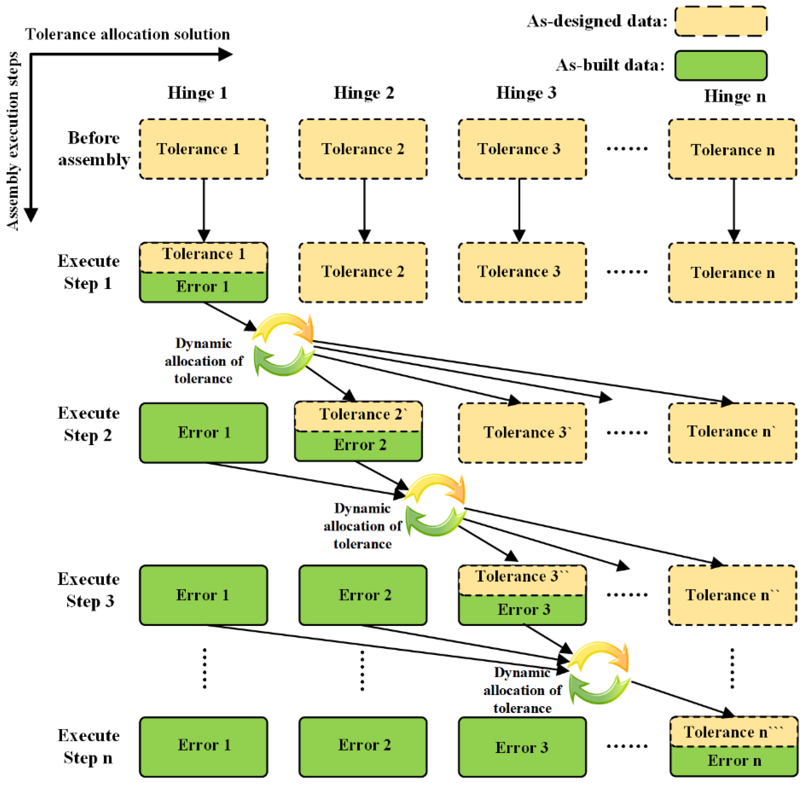
A tolerance dynamic allocation method based on the as-built data is proposed. This contribution aims to compensate for the last research gap mentioned above. The as-built data measured during the assembly process have considerable value for tolerance allocation. The proposed method can dynamically allocate tolerance for subsequent processes using the completed processes’ as-built data, which can relax the tolerance while guaranteeing the assembly quality. Therefore, it can reduce the assembly difficulty and cost. Of course, if the as-built data exceed the tolerance, the dynamic tolerance allocation model can be used to evaluate whether the current process should be reworked or to tighten the subsequent processes’ tolerances to ensure the final quality.

2. Influence Factors of Service Performance of LSDM

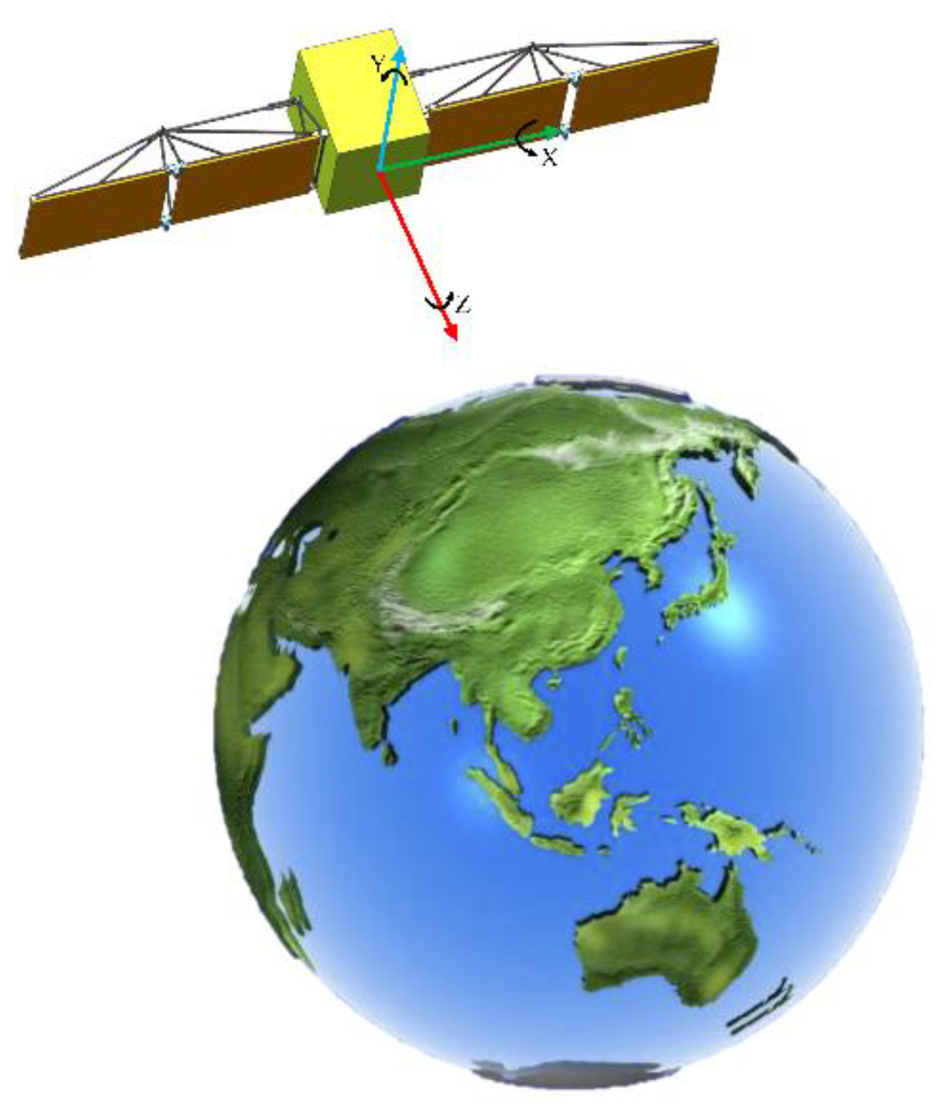
2.1. The Pointing Accuracy of Satellites in Space

Earth observation satellites are capable of imaging and remotely measuring Earth’s surface and of tracking and observing aerial and ground targets, as shown in Figure 2. To achieve precise target location observation, satellite antenna panels demand high pointing accuracy. The LSDM serves as the payload platform of the antenna panel. Its assembly quality is ultimately evaluated to ensure that the antenna panels’ pointing accuracy meets the service requirements during an in-orbit satellite mission. To guarantee alignment between the antenna panels and satellite body in space, ensuring the pointing accuracy between the normal vector of the antenna panels and the coordinate system of the satellite body during ground assembly is necessary.

As shown in Figure 3, to quantitatively analyze the pointing angle $\theta$, the normal vector of the antenna panel $\overrightarrow{N}$ should be projected onto the X-O-Z and Y-O-Z planes. The resulting angles between the projected vector and the Z-axis in each plane are, respectively, referred to as the yaw angle $\alpha$ and the pitch angle $\beta$. These parameters are critical for ensuring accurate alignment between the antenna panel and satellite body in space. The equivalent model of the projection angles is shown in Figure 3b, and the pointing angle $\theta$ can be expressed by the yaw angle $\alpha$ and pitch angle $\beta$:

$$\theta =\arccos \frac{1}{\sqrt{{\tan }^2\alpha +{\tan }^2\beta +1}}$$

(1)

2.2. The Influence Factors of Ground Assembly for Service Performance in Space

It can be inferred from Equation (1) that, when the $\alpha$ and $\beta$ are determined, the pointing angle $\theta$ of a satellite antenna panel will be uniquely determined. Therefore, during the assembly process, the LSDM can be projected onto the X-O-Z and Y-O-Z planes, respectively. By solving for $\alpha$ and $\beta$, the pointing angle $\theta$, which represents the satellite antenna panel’s pointing accuracy, can be calculated.

This paper provides a detailed explanation of the modeling of assembly errors and the allocation of tolerances using the LSDM of a satellite’s X+ side as an example. Figure 4 shows the schematic projection of an assembly site on the X-O-Z plane, and the letters from a to j represent the hinge components.

Gravity’s impact is the main difference in the LSDM’s service environment and its on-ground assembly environment. During ground assembly, gravity affects not only the deformation of individual parts but also the interaction between them. To minimize the mutual influence of parts caused by gravity during the assembly process, gravity unloading is implemented for each truss hinge, as shown in Figure 4. However, due to microgravity technology’s current limitations, it is not feasible to achieve a microgravity environment for all LSDM components. When gravity compensation is only applied to each truss hinge component, gravity’s primary impact on the LSDM assembly can be seen in two aspects:

(i)

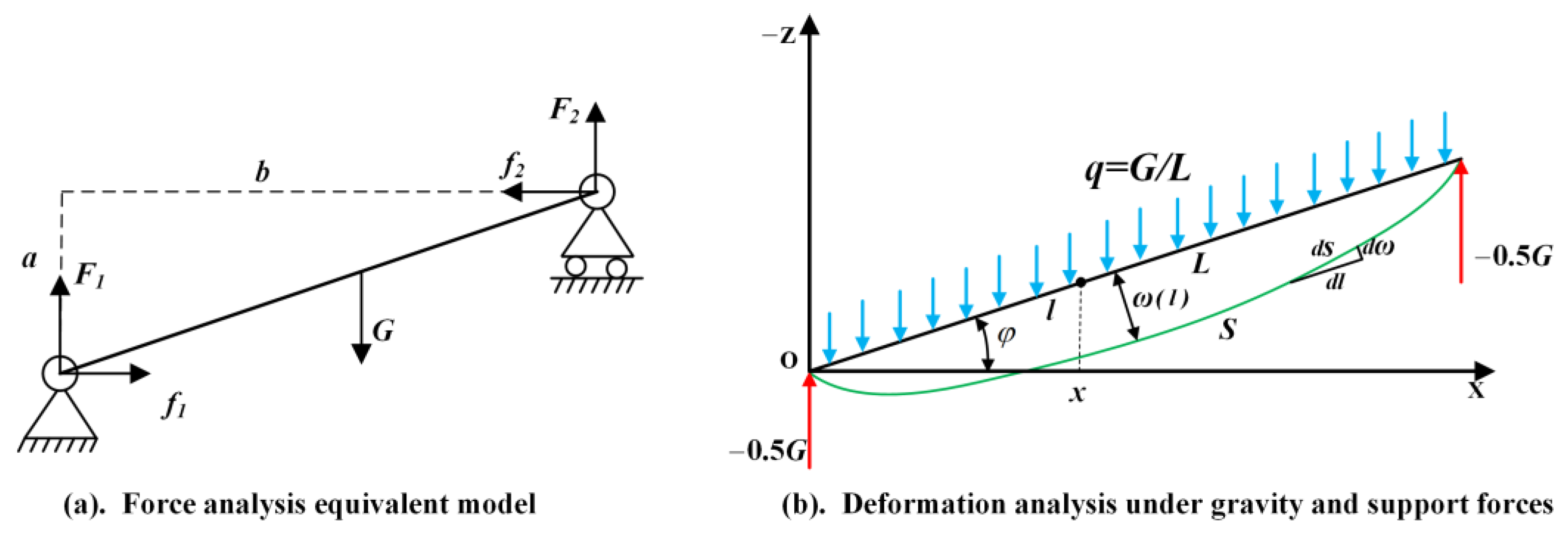
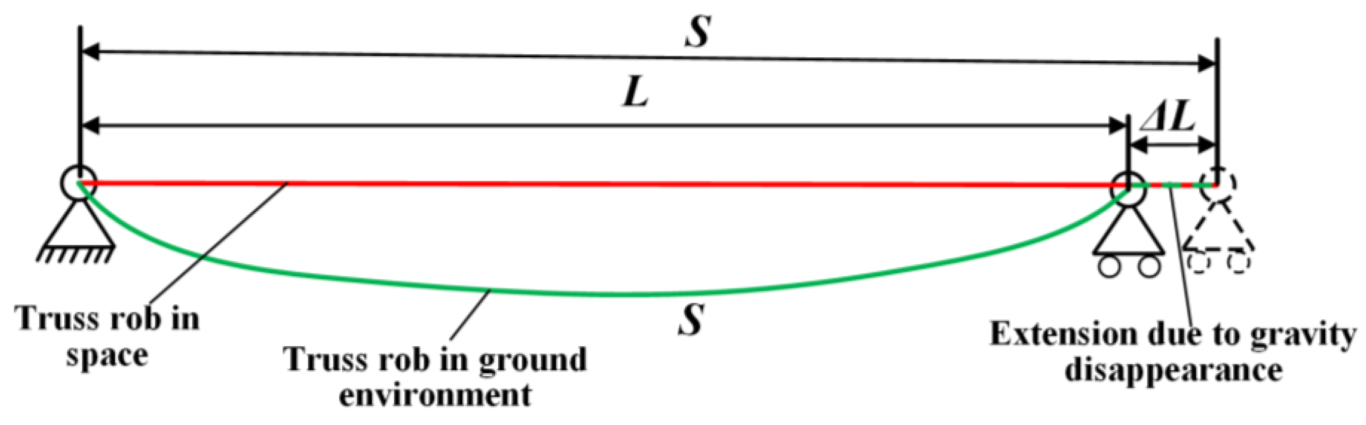
Deformation of the truss rod. The LSDM’s truss rods consist of carbon fiber and have a large length-to-diameter ratio. During ground assembly, except for the rods installed vertically, the other rods experience bending deformation due to gravity’s influence. When the LSDM is in the space environment where gravity is absent, the bending deformation tends to recover. However, this deformation recovery will affect the pointing accuracy.

(ii)

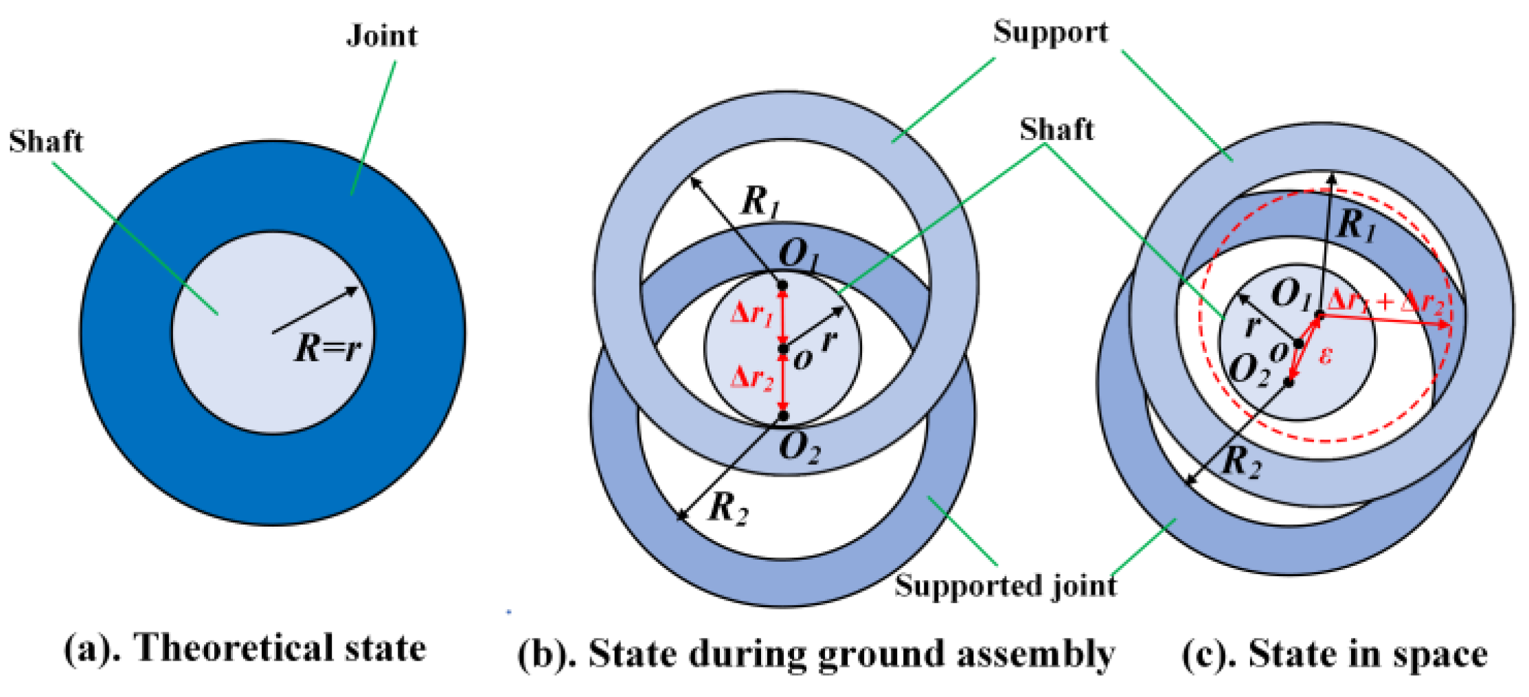
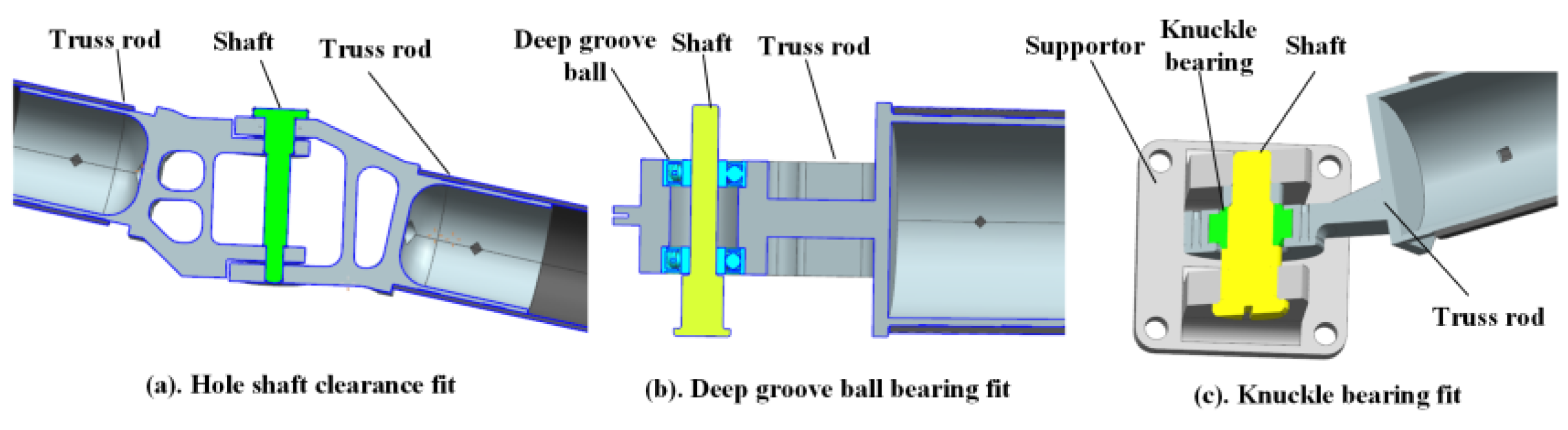
Clearance of truss hinge. The shaft and hole of the truss hinge usually have clearances. During ground assembly, the hole and shaft are in contact under gravity. However, when the gravity disappears in space, the contact will be changed, which will also affect the pointing accuracy.

To analyze the aforementioned factors’ impacts, this paper compares the differences between the ground assembly environment and service environment in space, which will provide a basis for constructing an assembly error model in the subsequent section.

2.3. Comparative Analysis of Truss Rod Deformation in Ground and Space Environment

To reduce the satellite’s overall mass, the LSDM’s truss rods usually consist of carbon fiber, which has low density, high strength, and high rigidity. However, due to their high length-to-diameter ratio, which can exceed 100, the truss rods are inevitably affected by gravity during ground assembly. In actual assembly, all truss hinges are implemented with gravity compensation, and the axial clearance between the truss rod and truss hinge is left. Therefore, the truss rod can be effectively modeled, as shown in Figure 5a.

By analyzing Figure 5a, it can be seen that $f_1$ and $f_2$ are both 0, while $F_1$ and are all $-0.5G$. Based on this information, the deformation analysis of the truss rod can be performed as shown in Figure 5b, which considers the gravity $G$ as a uniformly distributed load $q$.

As shown in Figure 5b, the truss rod’s theoretical length is $L$. The angle between the truss rod and the horizontal plane is $\phi ,\phi \in \left(-0.5\pi ,0.5\pi \right)$. The truss rod bends under uniform load $q$. The deflection can be expressed as $\omega \left(l\right)$,where the l is the length of the rod from 0 to x, and the value of l can be expressed as $\raisebox{1ex}{$x$}\!\left/ \!\raisebox{-1ex}{$\cos \phi $}\right.$. Then, the actual length of the truss rod can be calculated as follows:

$$S=\frac{L}{n}\left[\frac{1}{2}\left(\sqrt{1+\frac{G^2{L}^4{\cos }^2\phi }{64E^2{I}^2}}+\sqrt{1+\frac{25G^2{L}^4{\cos }^2\phi }{576E^2{I}^2}}\right)+{\displaystyle \sum _{i=1}^{n-1}\sqrt{1+\frac{G^2{\cos }^2\phi }{4E^2{I}^2}{\left(\frac{1}{3L}{l}_i^3+\frac{1}{2}{l}_i^2-\frac{1}{4}{L}^2\right)}^2}}\right]$$

(2)

where E is the elasticity modulus which is determined by the material of the truss rod; I is the inertia moment, which is related to the cross-sectional shape of the truss rod; n denotes dividing the length L into n segments; and $l_i$ can be expressed as follows:

$$\{\begin{array}{c}{l}_i=l_{i-1}+\frac{L}{n}\\ l_0=0\\ l_n=L\end{array}$$

(3)

Figure 6 shows that the rod’s length changes from the gravity environment to the service environment in space. The rod’s length changes from its nominal length L on the ground to its actual length S in space. The distance between the hinges at both ends of the rod changes from L to S, and the elongation $\Delta L$ can be expressed as follows:

$$\Delta L=S-L$$

(4)

2.4. Comparative Analysis of Hinge Clearance in Ground and Space Environments

Apart from the truss deformation, another important factor that affects the LSDM’s assembly quality is the hinge clearance.

The typical hinge’s forms of the LSDM are shown in Figure 7. Each hinge has a support due to gravity compensation at each hinge position during the ground assembly. The gravity compensation measures have three forms: (a) support, shaft, and supported joint; (b) support connected with a gravity compensation device, shaft, and supported joint; and (c) support connected with a gravity compensation device, shaft, and multi-supported joints.

The three types of hinge components are all assembled by measuring the shaft as the nominal position of the hinge. Additionally, according to Figure 5a, the hinge is only subjected to vertical forces, thus resulting in the shaft and hole only contacting in the vertical direction in the ground assembly process. However, the shaft and joints enter a state of suspension after the LSDM is sent to space, as shown in Figure 8c.

3. LSDM Assembly Error Model in Microgravity Assembly on the Ground

Section 2 analyzes the main factors that affect the LSDM’s performance from the perspectives of differences and similarities between the ground assembly and space service environments. These factors include the truss rod deformation under gravity and the clearance between the hinge shaft and hole. In addition, each hinge’s assembly position errors are also important factors that affect the final pointing accuracy. This section will construct a ground assembly error propagation model aimed at improving the LSDM’s service performance.

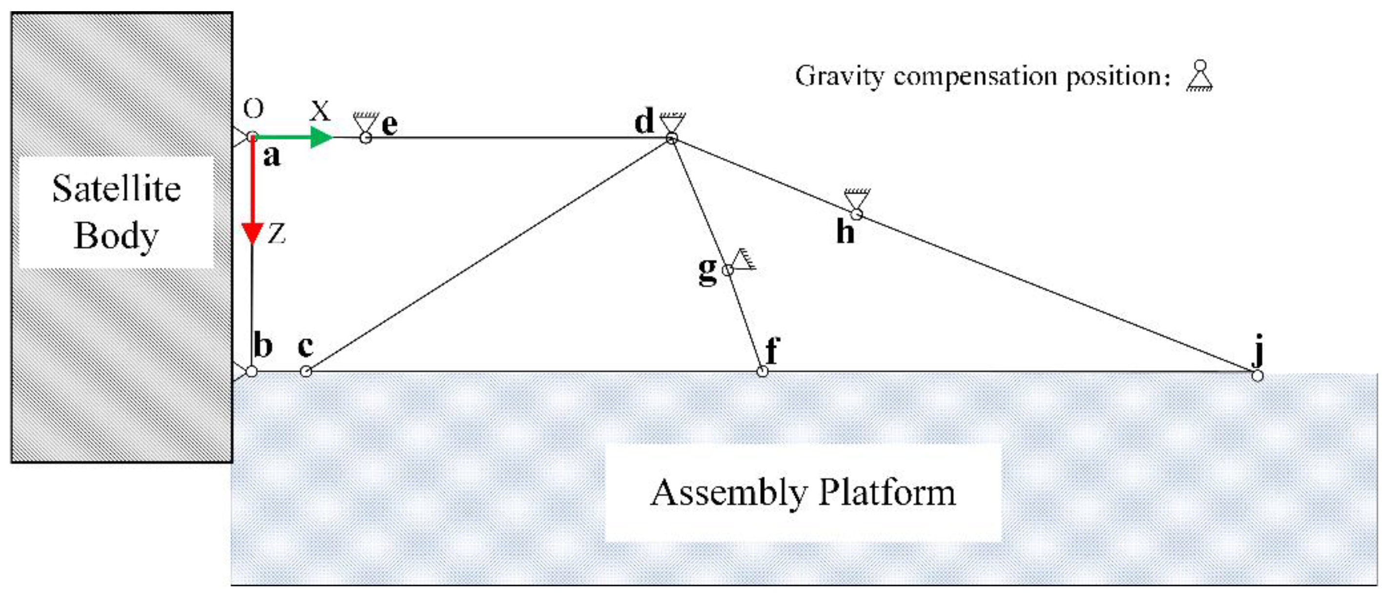
3.1. Characteristic Analysis for Truss Rod

As Figure 4 shows, the LSDM’s projection in the X-O-Z plane can be seen as a topological structure composed of multiple closed-loop chains, which mainly consists of hinges and truss rods. As

Table 1. Rod types of the LSDM.

Rod Types	Characteristic	Schematic Diagram
Independent Rod	The rod connects hinges at both ends, and the length between the two hinges is affected by rod deformation.
Coupling Rod	In addition to the hinge at both ends of the rod, there is also one or more hinges at the middle position, and the middle hinge is fixed to the rod.
Equivalent Fixed-Length Rod	The rod is determined by two supports fixed on the antenna panel or satellite body, and the rod is not affected by deformation.

shows, the rods can be divided into three types according to their connection forms, which is defined in this paper as the independent rod, coupling rod, and equivalent fixed-length rod. Their definitions are as follows:

(i)

Independent Rod. Each end of the rod connects to a hinge, and there is no hinge connected in the middle of the rod. This rod type is the most numerous in the LSDM.

(ii)

Coupling Rod. In addition to the hinge at both ends of the rod, there is also one or more hinges at the middle position, and the middle hinge is fixed to the rod. The coupled rod cannot fold around the middle hinge.

(iii)

Equivalent Fixed-Length Rod. The rod is determined by two supports fixed on the antenna panel or satellite body, and the distance between the two supports is not affected by the rod deformation.

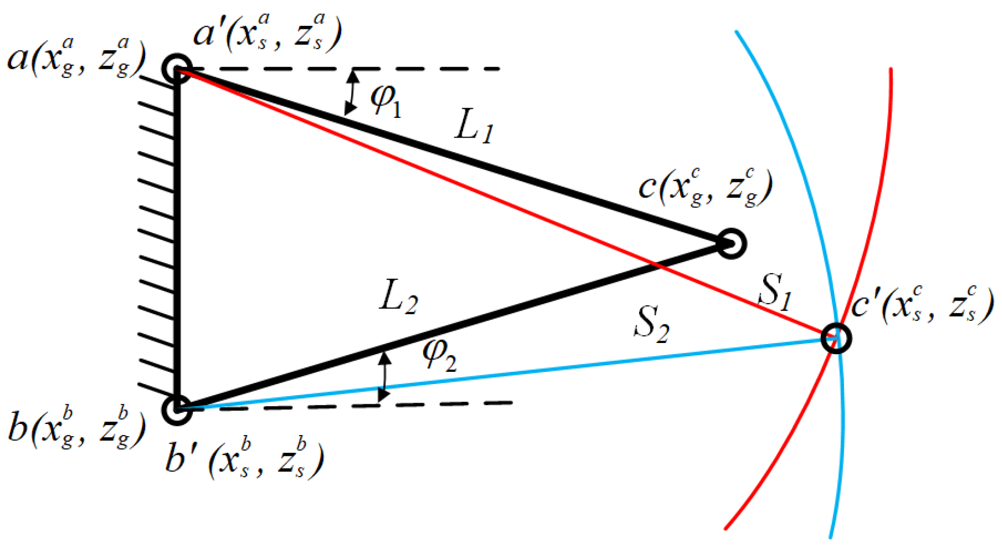
3.2. Assembly Error Propagation of Single-Loop Closed Chain

This section builds the assembly error propagation model in a single-loop closed chain and considers three factors: the assembly positioning error, the truss rod deformation, and the hinge clearance. The process of constructing an error model is progressive, which means that, initially, only the positioning error is considered and, then, hinge clearance effects are considered. Finally, all three factors are accounted for.

Assembly positioning error is inevitable during the assembly process. Typically, the assembly process instruction provides each hinge’s positional tolerance, and the operator uses a laser tracker to measure each hinge’s spatial position. Based on the given tolerance, the operator determines whether the hinge’s positioning error meets the process requirements. The hinge clearance fit states are shown in Figure 8. The state is stable on the ground, but the balance is broken in space. When considering the positioning error and hinge clearance, the hinge center coordinates in space are calculated as follows:

$$\{\begin{array}{l}{x}_s=x+\Delta x, \mathrm{support}\hfill \\ x_s=x+\Delta x+{\epsilon }_x, \mathrm{supported} \mathrm{joint}\hfill \\ z_s=z+\Delta z+\Delta r_1, \mathrm{support}\hfill \\ \begin{array}{l}{z}_s=z+\Delta z-\Delta r_2+{\epsilon }_z, \mathrm{supported} \mathrm{joint}\\ {\left(\Delta x\right)}^2+{\left(\Delta y\right)}^2\le {\xi }_{}{}^2\\ {\epsilon }_x\in \left[-\Delta r_1-\Delta r_2, \Delta r_1+\Delta r_2\right]\\ {\epsilon }_z\in \left[0, 2\Delta r_1+2\Delta r_2\right]\end{array}\hfill \end{array}$$

(5)

where $x_s$, $z_s$ are the hinge joint center coordinates in space, and they are not constant but vary within certain ranges; x, z represent the designed coordinates of the hinge; $\Delta x$ and $\Delta z$ represent the hinge’s positioning errors in the directions of X and Z, respectively; $\xi$ is the hinge’s positioning tolerance; $\Delta r_1$ is the clearance between shaft and support; $\Delta r_2$ is the clearance between shaft and supported joint; and ${\epsilon }_x$ and ${\epsilon }_z$ are the components of the center offset between the support and the supported joint in X direction and Z direction, respectively.

Equation (5) is the assembly error model considering the positioning error and clearance that has different states on the ground and in space. Then, the truss rod deformations should be considered in the above assembly error model.

A detailed analysis of the truss rod deformation is provided in Section 2.3. However, simply inserting the rods’ length changes into the assembly error model when there is coupling between rods is not feasible. In this paper, the truss rod deformation of the closed-chain structure is introduced into the assembly error model, as shown in Figure 9.

A closed-chain structure is composed of three or more truss rods connected by hinges. It contains at least one equivalent fixed-length rod. For the one without equivalent fixed-length rods, the known lengths of the truss rods determined by the previous closed-chain can be used as the equivalent fixed-length rod for the current closed chain.

As shown in Figure 9, the three center coordinates of the hinges are $\left(x_g^a,z_g^a\right),\left(x_g^b,z_g^b\right),\left(x_g^c,z_g^c\right)$ when considering the positioning error and clearance in the ground assembly. Therefore, the two independent rods’ lengths can be expressed as follows:

$$\{\begin{array}{l}{L}_1=\sqrt{{\left(x_g^c-x_g^a\right)}^2+{\left(z_g^c-z_g^a\right)}^2}\\ L_2=\sqrt{{\left(x_g^c-x_g^b\right)}^2+{\left(z_g^c-z_g^b\right)}^2}\end{array}$$

(6)

The lengths of the rods in space that are labelled as $S_1,S_2$ can be obtained using Equation (2). The position of hinge c in space is not simply determined by only extending a single rod. It is determined by the intersection of two circles with the starting points of the two rods a and b as the center of the circle and the extended rod lengths $S_1,S_2$ as the radii. There are usually two intersection points for the two circles. The point closer to the original c point is the actual position caused by the rod length change in space. Based on the above analysis, the calculation of point c is as follows:

$$\{\begin{array}{l}{\left(x_s^c-x_s^a\right)}^2+{\left(z_s^c-z_s^a\right)}^2=S_1^2\\ {\left(x_s^c-x_s^b\right)}^2+{\left(z_s^c-z_s^b\right)}^2=S_2^2\end{array}$$

(7)

The solution can be expressed as follows:

$$\{\begin{array}{l}{x}_s^c=\frac{-b_2\pm \sqrt{b_2^2-4a_1{c}_3}}{2a_1}\hfill \\ z_s^c=c_2-b_1{x}_s^c\hfill \end{array}$$

(8)

where the constant terms can be expressed as follows:

$$\{\begin{array}{l}{a}_1=1+b_1^2\hfill \\ b_1=\frac{x_s^b-x_s^a}{z_s^b-z_s^a}\hfill \\ b_2=-2x_s^a-2b_1\left(c_2-z_s^a\right)\hfill \\ c_1=S_1^2-S_2^2+{\left(x_s^b\right)}^2-{\left(x_s^a\right)}^2+{\left(z_s^b\right)}^2-{\left(z_s^a\right)}^2\hfill \\ c_2=\frac{c_1}{2\left(z_s^b-z_s^a\right)}\hfill \\ c_3={\left(x_s^a\right)}^2+{\left(c_2-z_s^a\right)}^2-S_1^2\hfill \end{array}$$

(9)

The point closer to the initial point c is chosen as the c′ that is the point in space considering the three effect factors including the positioning error, hinge clearance, and truss rod deformation as follows:

$$c^{\prime }\left(x_s^c,z_s^c\right)=\arg \min \left\{{\left(x_{s\_1}^c-x_g^c\right)}^2+{\left(z_{s\_1}^c-z_g^c\right)}^2,{\left(x_{s\_2}^c-x_g^c\right)}^2+{\left(z_{s\_2}^c-z_g^c\right)}^2\right\}$$

(10)

where $\left(x_{s\_1}^c,z_{s\_1}^c\right)$, $\left(x_{s\_2}^c,z_{s\_2}^c\right)$ are the solutions of Equation (7). Thus, the assembly error model of the single-loop closed-chain structure is constructed.

3.3. Assembly Error Propagation of Multi-Loop Closed Chain

Based on the above analysis, the center coordinates of each hinge of the single loop closed chain structure under the influence of the three error factors can be calculated. The LSDM can be equivalent to the combination of multiple single-loop closed chains, as shown in Figure 10. I, II, and III are used to represent the three closed loop chains, respectively, and the assembly error propagates among the closed loops.

The coordinates of hinges c and d in space can be solved in loop I, and then, the truss rod cd can be seen as the equivalent fixed length rod for the assembly error solving of loop II, as well loop III eventually being solved. Then, the coordinates of all the truss hinges in space in the weightless environment can be obtained.

The LSDM’s yaw angle $\alpha$ in space is as follows:

$$\alpha =\frac{\pi }{2}-\arccos \frac{\overrightarrow{\mathrm{cj}}\cdot \overrightarrow{\mathrm{ab}}}{\overrightarrow{\left|\mathrm{cj}\right|}\times \left|\overrightarrow{\mathrm{ab}}\right|}$$

(11)

where the vectors in the above equation can be expressed as follows:

$$\{\begin{array}{c}\overrightarrow{\mathrm{ab}}=\left(x_s^b-x_s^a,z_s^b-z_s^a\right)\\ \overrightarrow{\mathrm{cj}}=\left(x_s^j-x_s^c,z_s^j-z_s^c\right)\end{array}$$

(12)

Thus, the error propagation model for the yaw angle $\alpha$ affected by the three factors—positioning error, hinge clearance, and truss rod deformation in the X-O-Z plane—can be established. Similarily, the same method can be used to build the error propagation model of the pitch angle $\beta$ in X-O-Y plane. Then, the pointing angle $\theta$ can be calculated using Equation (1).

Finally, the relationship between the positioning error of the ground assembly and the pointing accuracy in space can be established, which is used to guide the assembly operations for the workers, and it provides a basis for the dynamic tolerance optimization in the subsequent sections.

4. Dynamic Tolerance Allocation Based on As-Built Data

4.1. Dynamic Tolerance Allocation Flow among Assembly Processes

The LSDM’s pointing angle $\theta$ in space is an index on the service performance. According to the assembly error model built in the previous section, the factors that affect the pointing accuracy include the positioning error, hinge clearance, and truss rod deformation. The hinge clearance is determined by the parts’ manufacturing accuracy. In the assembly stage, the accurate fit clearance can be obtained by measuring the size of the hole and shaft. The rod deformation can be calculated by the rod length and the angle between the rod and the horizontal plane. Therefore, the tolerance allocation refers to the allocation of the positioning accuracy tolerance for each hinge.

The above sections provide the assembly error propagation model for improving the LSDM’s service performance. Additionally, each assembly process’ tolerance can be divided according to the error propagation model. In the traditional assembly error mode, the tolerance allocation scheme is allocated before assembly, and it usually remains unchanged during the entire assembly process. However, this mode ignores the usefulness of the as-built data, which is uneconomical for assembly.

In this paper, a dynamic allocation method of assembly tolerance based on the as-built data is proposed. The tolerance dynamic allocation flow is shown in Figure 11. Before the assembly task starts, the process planner provides an initial tolerance allocation solution that can meet the product performance requirements based on experience. During the assembly process, the components corresponding to the operation will determine an actual error value within the design tolerance. Based on the completed process’ actual error value, which is called the as-built data, the dynamic allocation of the subsequent tolerance is realized by the GA. Generally, the as-built data are not the boundary value of the tolerance, so subsequent tolerances can usually be expanded to reduce the assembly difficulty and costs. However, when the as-built data are close to the tolerance boundaries or occasionally exceed the tolerance, this method ensures the final assembly quality by reducing the tolerances in subsequent processes in time.

4.2. Optimal Tolerance Allocation Based on GA and As-Built Data

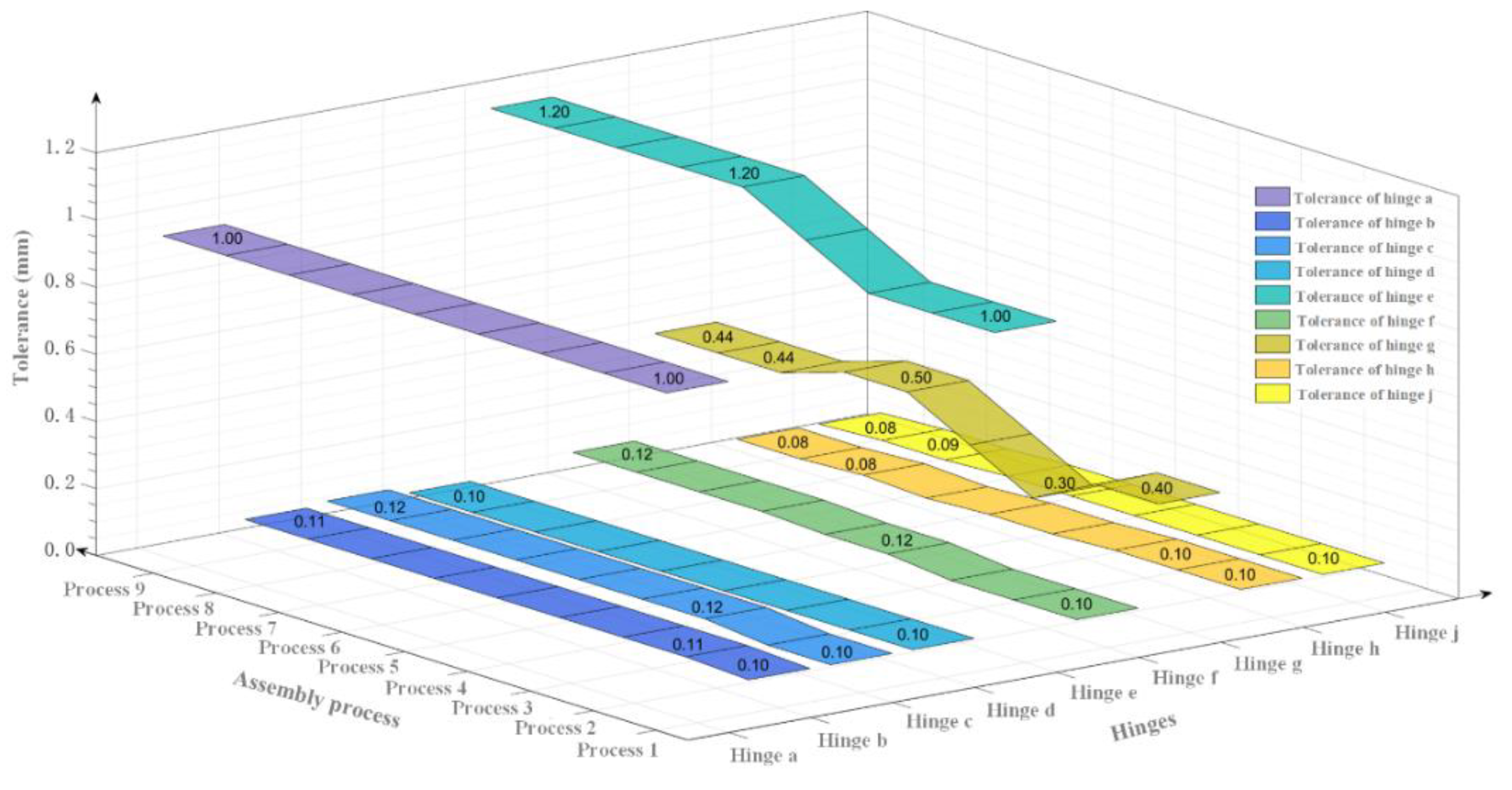
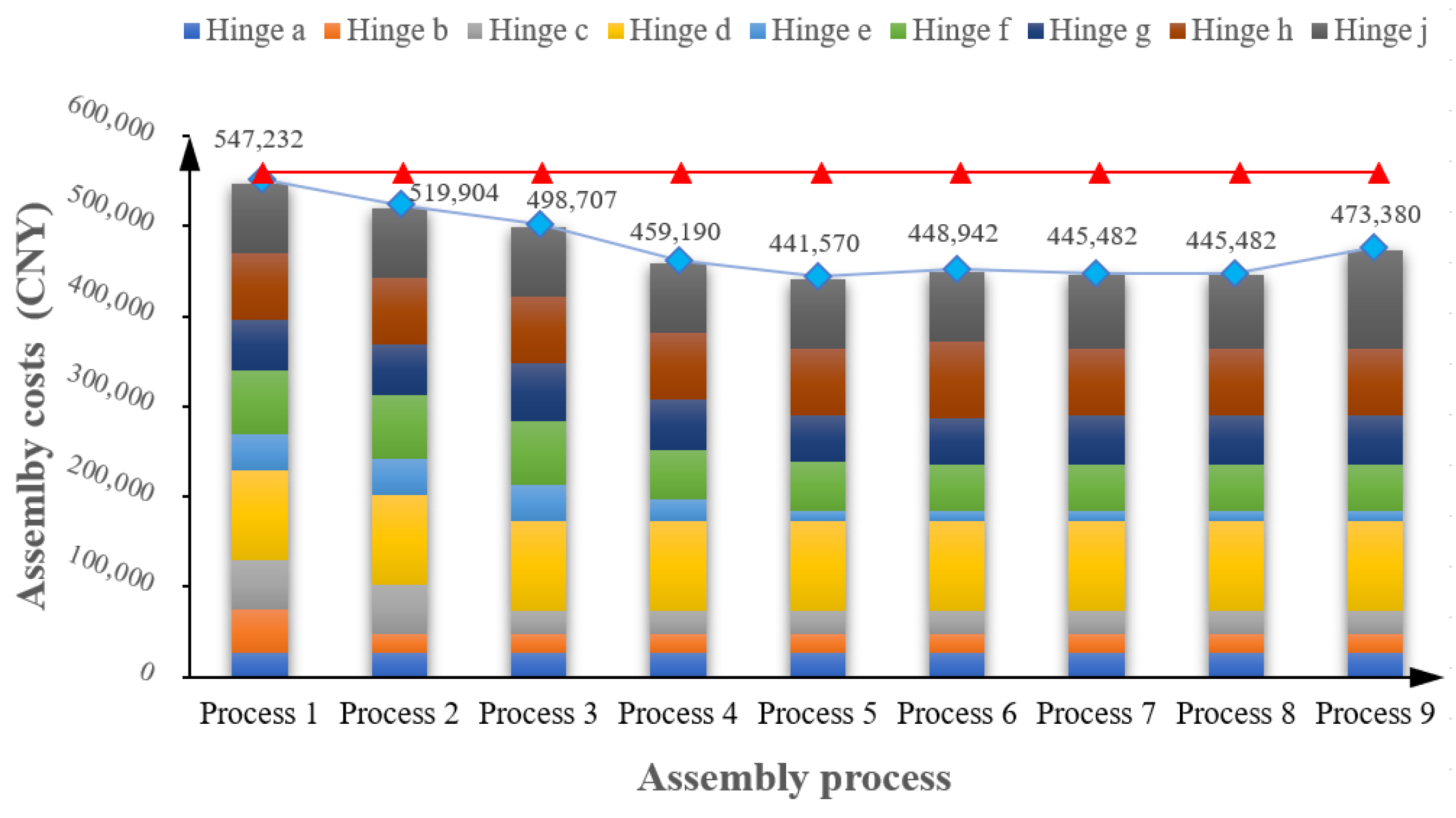
The GA is used to optimize the tolerance allocation, which takes the as-built data as the input. The flow of GA optimizing tolerance is shown in Figure 12, which contains four modules: the initialization, fitness evaluation, genetic evolution, and tolerances update.

Initialization: The dimension chains are generated according to the LSDM’s structure, and the tolerance schemes are allocated to each process link of the assembly process dimension chain using the Monte Carlo method according to the service-positioning accuracy and error propagation model. The feature information of each tolerance allocation scheme is extracted and coded to form the initial population.

Fitness evaluation: By calculating each chromosome’s fitness, the superior individuals are filtered out from the population and the iteration is terminated according to the termination conditions.

Genetic evolution: The selection of, crossover of, and variation in each chromosome in the population are carried out to inherit and produce more individuals conforming to the fitness function and to realize the positive evolution of the population. The genes on the chromosome are divided into two categories in the proposed method. They are genes encoded by as-built data and genes encoded by tolerance ranges. The genes of as-built data are selected to the next generation directly without crossover and variation.

Tolerances update: The evolutionary loop that satisfies the termination conditions terminates the iteration, outputs the optimal tolerance allocation scheme, and updates the dimension chain to the next step of the assembly tolerance allocation.

To achieve chromosome coding, each tolerance scheme is treated as a chromosome. The as-built data of completed processes and the unassembled hinges’ position tolerances are treated as the genes to obtain the chromosome coding form as follows:

$$X_i^j=\left({\lambda }_1^j\dots {\lambda }_e^j\dots {\lambda }_{i-1}^j,{\xi }_i^j\dots {\xi }_m^j\dots {\xi }_n^j\right)$$

(13)

where $X_i^j$ represents the j-th tolerance scheme for the i-th assembly process, when the first (i − 1)-th processes have been completed; ${\lambda }_e^j$ is the as-built data of the e-th assembly process; and ${\xi }_m^j$ represents the m-th process’ position tolerance.

The fitness design is essential in GA for tolerance dynamic optimization. This paper designs the fitness function from three dimensions: the service performance, the assembly costs, and the population’s diversity.

For the service performance, the assembly error model built in Section 3 is used as the fitness function. For the convenience of expression, the error model’s function is defined as follows:

$${\theta }_i^j=f\left({\lambda }_1^j\dots {\lambda }_e^j\dots {\lambda }_{i-1}^j,{\xi }_i^j\dots {\xi }_m^j\dots {\xi }_n^j\right)$$

(14)

where ${\theta }_i^j$ represents the pointing accuracy corresponding to the j-th tolerance scheme in the i-th assembly process. Assume that the LSDM’s pointing accuracy must be no more than ${\theta }_s$; then, the fitness function considering the service performance is as follows:

$${\theta }_i^j\le {\theta }_s$$

(15)

In general, the assembly cost and service performance are mutually constrained, and the pursuit of the maximum service performance is bound to result in a sharp increase in cost. Therefore, it is necessary to consider the cost constraints when using GA to optimize the tolerances. To ensure the calculation accuracy and to simplify the calculation, this paper uses the quintic polynomial model to construct the assembly cost-tolerance model. The product assembly cost $C_j$ corresponding to the j-th tolerance scheme adopts the McLaurin series and the quintic cost function equation as follows [31]:

$$\{\begin{array}{l}{C}_j={\displaystyle \sum _{i=1}^n{C}_j\left({\xi }_i^j\right)}\hfill \\ C_j\left({\xi }_i^j\right)=a_0+a_1{\xi }_i^j+a_2{\left({\xi }_i^j\right)}^2+a_3{\left({\xi }_i^j\right)}^3+a_4{\left({\xi }_i^j\right)}^4+a_5{\left({\xi }_i^j\right)}^5\hfill \end{array}$$

(16)

where $a_0,a_1,a_2,a_3,a_4,a_5$ are the cost parameters related to the tolerance variation. Their values can be obtained by calculating the cost of labor for each process and fitting the assembly cost curve.

In addition, to avoid the GA falling into local optimum due to being “premature”, this paper introduces the population diversity’s constraints into the fitness function. Based on the tolerance’s attribute, the mean of the gene dispersion degree at the corresponding chromosome location in a population is defined as the diversity $R$ as follows:

$$\{\begin{array}{c}R=\frac{1}{n}{\displaystyle \sum _i^n{S}_i^2}\\ S_i^2=\frac{1}{m-1}{\displaystyle \sum _{j=1}^m\left({\xi }_i^j-\overline{{\xi }_i^{}}\right)}\end{array}$$

(17)

In summary, the fitness function’s purpose is to select individuals in the population who have the skills to meet the product’s service performance and have better assembly economy.

5. Case Study

5.1. Experimental Setup

To prove the method’s effectiveness, a single wing LSDM structure is used to validate the application of the assembly error model and dynamic tolerance allocation in the ground assembly process. As shown in Figure 13, there are nine sets of truss hinges in the LSDM. Additionally, each set of truss hinge typically exists in pairs that have coincident projections in the X-O-Z plane. Figure 13c shows the actual assembly scene of the LSDM. The parallel robot and the collaborative robot are used to realize the microgravity for the hinges. A laser tracker is used to measure each hinge’s spatial coordinates. The coordinate system is first established with its origin point at the center of hinge a and the positive of the Z-axis along the normal direction of the satellite antenna plate to the ground. Then, the theoretical coordinates and initial tolerance of each hinge are shown in

Table 2. The designed coordinates and initial tolerances of the hinges in X-O-Z plane.

Hinges	X Designed Coordinates	Z Designed Coordinates	X Initial Tolerances	Z Initial Tolerances
a	0.000	0.000	±0.5	±0.5
b	32.000	1225.000	±0.5	±0.05
c	167.006	1220.008	±0.5	±0.05
d	2540.581	−139.011	±0.05	±0.5
e	449.138	−24.575	±0.5	±0.5
f	2692.000	1230.000	±0.5	±0.05
g	2627.721	648.845	±0.2	±0.2
h	2999.851	68.252	±0.05	±0.5
j	5552.000	1220.001	±0.5	±0.05

.

According to Section 2, for each truss rod ‘s length and mass, the angle between the rod and the horizontal plane affect the rod’s elongation. The projected rod length, the equivalent mass, and the theoretical value of the angle between the rod and X-axis are shown in

Table 3. Projected length, equivalent mass, and angle between rod and X-axis in X-O-Z plane.

Truss Rod	Projected Length (mm)	Equivalent Mass (kg)	Angle between Rod and X-axis
ab	1231.387	0.688	90.000°
bc	135.099	0.075	0.000°
cd	2735.103	1.528	−29.794°
ed	2094.571	1.170	−3.132°
ae	449.810	0.251	−3.132°
cf	2525.013	1.4106	0.000°
fg	584.699	0.327	83.689°
dg	792.660	0.443	83.689°
fj	2860.017	1.598	0.000°
hj	2799.998	1.564	24.289°
dh	503.872	0.281	24.289°

.

Another factor of the assembly error model in this paper is the hinge clearance. As shown in Figure 14, there are three hinge types in the LSDM, and the different types have different clearances, as shown in

Table 4. Hinge clearances in the LSDM.

Close Loop	Hinge	Components	Nominal Diameter (mm)	Fit Type	Clearance Range (mm)
I	a	ab rod	6	Hole–shaft clearance fit	+0.024 +0.004
		a shaft	6
			5	Deep groove ball bearing fit	+0.013 +0.002
		ae rod	5
	b	ba rod	8	Hole–shaft clearance fit	+0.029 +0.005
		b shaft	8
			8	Hole–shaft clearance fit	+0.029 +0.005
		bc rod	8
	c	cb rod	10	Hole–shaft clearance fit	+0.029 +0.005
		c shaft	10
			12	Knuckle bearing fit	+0.032 +0.008
		cd rod	12
	d	dc rod	12	Knuckle bearing fit	+0.032 +0.008
		d shaft	12
			12	Deep groove ball bearing fit	+0.018 +0.003
		de rod	12
	e	ea rod	11	Hole–shaft clearance fit	+0.035 +0.006
		e shaft	11
			7	Deep groove ball bearing fit	+0.013 +0.002
		ed rod	7
II	c	cd rod	12	Knuckle bearing fit	+0.032 +0.008
		c shaft	12
			10	Hole–shaft clearance fit	+0.029 +0.005
		cf rod	10
	e	dc rod	12	Knuckle bearing fit	+0.032 +0.008
		d shaft	12
			12	Knuckle bearing fit	+0.032 +0.008
		dg rod	12
	g	gd rod	10	Hole–shaft clearance fit	+0.029 +0.005
		g shaft	10
			10	Hole–shaft clearance fit	+0.029 +0.005
		gf rod	10
	f	fg rod	12	Knuckle bearing fit	+0.032 +0.008
		f shaft	12
			12	Knuckle bearing fit	+0.032 +0.008
		fc rod	12
III	d	dg rod	12	Knuckle bearing fit	+0.032 +0.008
		d shaft	12
			12	Knuckle bearing fit	+0.032 +0.008
		dh rod	12
	g	gd rod	10	Hole–shaft clearance fit	+0.029 +0.005
		g shaft	10
			10	Hole–shaft clearance fit	+0.029 +0.005
		gf rod	10
	f	fg rod	12	Knuckle bearing fit	+0.032 +0.008
		f shaft	12
			10	Hole–shaft clearance fit	+0.029 +0.005
		fj rod	10
	j	jh rod	12	Knuckle bearing fit	+0.032 +0.008
		j rod	12
			10	Hole–shaft clearance fit	+0.029 +0.005
		jf rod	10
	h	hd rod	10	Hole–shaft clearance fit	+0.029 +0.005
		h shaft	10
			10	Hole–shaft clearance fit	+0.029 +0.005
		hj rod	10

.

According to the previous analysis, the dynamic tolerance allocation method can reduce the assembly cost; to verify its authenticity, the assembly cost is counted in this paper. The quintic cost function Equation (16) uses the statistical data, and the cost coefficients of each hinge assembly are obtained as shown in

Table 5. LSDM assembly cost parameters.

Hinge	Assembly Cost Parameters
	a0	a1	a2	a3	a4	a5
a	3.3452 × 105	−1.4498 × 106	3.1431 × 106	−3.3891 × 106	1.7069 × 106	−3.1847 × 105
b	8.6004 × 105	−5.2956 × 107	1.3240 × 109	−1.5006 × 1010	7.6952 × 1010	−1.4459 × 1011
c	3.5005 × 105	−9.3720 × 106	1.1645 × 108	−5.2197 × 108	−7.0956 × 108	6.9301 × 109
d	5.7258 × 105	−2.7379 × 107	8.0764 × 108	−1.2285 × 1010	8.5116 × 1010	−2.0389 × 1011
e	5.3239 × 105	−2.79438 × 106	6.6941 × 106	−7.5263 × 106	3.8618 × 106	−7.2724 × 105
f	4.6480 × 105	−1.9256 × 107	4.7950 × 108	−6.4982 × 109	4.2035 × 1010	−9.6909 × 1010
g	2.1534 × 105	−1.2744 × 106	4.1364 × 106	−6.5950 × 106	4.8727 × 106	−1.3144 × 106
h	7.0081 × 105	−4.8295 × 107	1.7002 × 109	−2.8377 × 1010	2.0653 × 1011	−5.0759 × 1011
j	4.2933 × 105	−2.1676 × 107	6.9152 × 108	−1.1127 × 1010	7.9729 × 1010	−1.9453 × 1011

.

In addition, to guide the assembly process, tolerance dynamic allocation software is developed using the Unity 3D platform, and the assembly error model considering the service performance presented in this paper is integrated into the software. The core interface of the developed software is shown in Figure 15.

5.2. Experimental Results and Analysis

In this paper, the differences between the existing method and the proposed method are compared and analyzed from two aspects: pointing accuracy and assembly cost.

5.2.1. Pointing Accuracy Analysis

The pointing accuracy’s error bar is used to express the different results under different assembly methods, as shown in Figure 16. The antenna’s pointing accuracy is affected by various factors such as the assembly positioning error, hinge clearance, and rod distortion. The pointing accuracy cannot be precisely determined before the assembly is completed because each hinge’s positioning error is not definite until the assembly is completed, though it is in a certain tolerance range. Moreover, the antenna’s actual pointing accuracy in space is almost impossible to measure directly when measured by humans on the ground. However, it can be indirectly predicted using methods such as the assembly error model that uses the hinges’ positioning error as the input and the pointing angle as the output. Therefore, the antenna’s pointing accuracy in space can be predicted using the assembly error model built in Section 3. As the assembly progresses, the pointing accuracy’s range is gradually decreased, but it does not eventually become a definite value because each hinge center in space is uncertain when hinge clearances are exists.

As shown in Figure 16, the pointing accuracy is predicted using the assembly error model built in Section 3. For the assembled hinge, the positioning error measured using the laser tracker is an input for the assembly error model. For the not-yet-assembled hinge, the tolerance is an input for the assembly error model. The blue error bars represent the antenna pointing accuracy using the previous method, regardless of gravity’s effect during ground assembly. Additionally, the orange error bars represent the antenna’s pointing accuracy using the assembly error model proposed in this paper, which considers the different environments between the ground assembly and service in space. Both methods perform gravity compensation for the LSDM’s key components. There is an initial error of 0.003° at the beginning of assembly when using the previous assembly method, which is caused by the gravity during the ground assembly. Additionally, the antenna’s pointing accuracy can be improved from 0.068° to 0.045° using the method proposed in this paper.

5.2.2. Assembly Cost Analysis

A truss hinge’s assembly cost is largely affected by the tolerance of the more rigorous direction. Figure 17 shows each hinge’s minimum tolerance during the assembly process, and the axis “Hinges” represents the LSDM’s hinge, while the axis “Assembly process” represents the assembly steps that are expressed by the process number. The tolerances are allocated to all the hinges at each step. Figure 17 shows the tolerance change as the assembly progresses.

Figure 18 shows each hinge’s tolerances allocated by the dynamic allocation method and the previous method. More than half of the hinges have looser tolerances allocated by the proposed method than the previous method. This indirectly shows that the dynamic tolerance allocation can reduce the assembly difficulty and cost.

Figure 19 shows the LSDM’s assembly cost when assembled by different method. The values in the figure are calculated using the quintic cost function in Equation (16) and the tolerances allocated in each assembly process. The horizontal axis represents the assembly process expressed by the process number. The vertical axis represents the cost calculated from the tolerance allocated to each hinge. Each process calculates the cost of all hinges of the LSDM. The bar of each process represents the total cost of the corresponding tolerance scheme, and the short bars with different colors mean the cost of different hinges. For the dynamic tolerance allocation method, the unassembled hinge’s tolerance can be changed during assembly. Thus, the length of the corresponding short bar changes with the assembly process. The assembled hinge’s tolerance will not be reallocated. Thus, the corresponding short bar remains unchanged. The total cost of the first process (Process 1) represents the cost under initial tolerance of the proposed method, and it is the same as the tolerance allocated by the previous method, which takes place before assembly and remains unchanged during assembly. As assembly progresses, the tolerances are continuously optimized by the proposed method, and the calculated assembly costs change accordingly. When the last process (Process 9) is executed, all tolerances have been optimized, and they are actual execution values, so the corresponding assembly costs can be viewed as actual execution costs of the proposed method. Comparing these, the assembly cost can be reduced from CNY 547,232 to CNY 473,380 using the dynamic tolerance allocation method, which represents a cost reduction rate of 13.5%.

6. Discussion

Compared with existing methods, the contribution of the assembly error modeling method proposed in this paper is that introduces the impact of gravity on the truss rod and hinge’s clearance into the model. The relationship between assembly error and service performance is established. Previous methods for reducing the impact of gravity include various advanced gravity compensation technologies. However, they are almost completely unable to unload the gravity of all the LSDM’s components for a long time. The proposed method considers the gravity changes between ground assembly and service in space on the premise of gravity compensation. Compared with previous methods, it further reduces the impact of gravity during assembly on service performance. The verification results presented in Figure 16 show that the proposed method can improve the pointing accuracy from 0.068° to 0.045°.

In addition, the dynamic tolerance allocation based on as-built data proposed in this paper is different from the previous method, which is completed before starting the assembly task and remains unchanged during the whole assembly process. To ensure the final quality, a limit situation is considered in the previous method, i.e., the final quality should be guaranteed even if the assembly error of each process reaches the tolerance boundary. However, in the actual assembly process, the error of each process does not usually reach the boundary but is better than it in most cases. Therefore, the as-built data measured during assembly has considerable value in tolerance allocation. The proposed method uses the as-built data as the input to dynamically allocate the tolerance of each process, which can relax tolerance while guaranteeing assembly quality. Thus, it can reduce assembly difficulty and cost. A comparison of the assembly costs is shown in Figure 19. Compared with the previous method, the dynamic tolerance allocation method reduces the LSMD assembly cost from CNY 547,232 to CNY 473,380. Moreover, if the as-built data exceed the tolerance, it can be used to evaluate whether the current process should be reworked or the subsequent processes’ tolerances should be tightened to ensure the final quality in service performance.

However, there are some limitations in this proposed method. For the assembly error model, only gravity’s impact is considered; even though it is the most important factor affecting the LSDM’s service performance, some other factors that have differences between ground assembly and service in space, such as temperature, radiation, and air pressure, are not yet considered in this method. Introducing those factors into the assembly error model, which could be studied in the future, may improve the proposed method and make the predicted pointing accuracy more accurate. Additionally, only GA is used for tolerance optimization in the dynamic tolerance allocation method. Besides GA, there are some other metaheuristic algorithms that could be used in the proposed method. Although it has achieved good results in reducing assembly difficulty and cost with the help of GA, this paper does not compare the effectiveness using different optimization algorithms. In the future, different optimization algorithms can be used to the proposed method, which may improve the LSDM assembly performance.

7. Conclusions and Future Work

This paper proposed the methods of assembly error modeling and tolerance dynamic allocation for the LSDM. The assembly error model is based on gravity compensation during the assembly process, and the different environments between the ground assembly and service in space are considered. Gravity variation is regarded as the core influencing factor. The changes in the hinge clearance and truss rod length caused by gravity variation are accounted for in the assembly error model to reduce gravity’s impact on the service performance. The tolerance dynamic allocation method uses the as-built data measured in the actual assembly process as the input. Compared with the previous fixed tolerance allocation methods, it can relax the tolerance while ensuring the quality, which can reduce the assembly difficulty and cost. In addition, if the as-built data exceed the tolerance, it can evaluate whether the current process should be reworked or the subsequent processes’ tolerances should be tightened to ensure the final quality.

Specifically, the differences between the ground assembly and service environments in space for the LSDM were analyzed, and the truss rod deformation and hinge clearance caused by gravity were regarded as factors affecting the satellite’s service performance; thus, an assembly error model to improve the service performance was built. The LSDM assembly based on the assembly error model proposed in this paper can improve the antenna pointing accuracy from 0.068° to 0.045°. To reduce the assembly cost and to improve the collaboration of the tolerance allocation between each process, the dynamic tolerance allocation method is proposed, which uses GA as the optimization algorithm and the as-built data as the input. In GA’s fitness function, the assembly error model built in this paper was constructed as the restrictive condition for the satellite’s service performance, and the assembly cost function of each assembly process was considered. The verification results show that this method can reduce the assembly cost by 13.5% while guaranteeing assembly quality.

Although this study achieved good verification results, some work remains to achieve more accurate satellite performance in space. For instance, this paper only considers the differences in gravity between the ground and space, which are the important influencing factors for assembly. However, there are also many other factors that affect the satellite’s final service performance, such as air pressure, radiation, and temperature. In the future, analyzing multi-physical coupling factors’ influences on the assembly quality using multi-physical simulation technology will have great potential. Additionally, optimization algorithms are of great significant for the tolerance allocation. Metaheuristic methods besides GA, such as the simulated annealing algorithm (SAA), ant colony optimization (ACO), particle swarm optimization (PSO), etc., can also be used as an optimization algorithm to improve the dynamic tolerance allocation method proposed in this paper.

References

1. Choi, H.; Kim, D.; Park, J.; Lim, J.H.; Jang, T.S. Modeling and Validation of a Passive Truss-Link Mechanism for Deployable Structures Considering Friction Compensation with Response Surface Methods. Appl. Sci. 2022, 12, 451. [Google Scholar] [CrossRef]
2. Chen, X.; Xu, Y.; Lin, Q.; Wang, X.; Li, L.; Cong, Q.; Pan, B. Mechanism design and dynamic analysis of a large-scale spatial deployable structure for space mission. In Proceedings of the SPIE 10322, Seventh International Conference on Electronics and Information Engineering, Nanjing China, 17–18 September 2016; Volume 1032226. [Google Scholar]
3. Li, H.Q.; Liu, X.F.; Guo, S.J.; Cai, G.P. Deployment dynamics and control of large-scale flexible solar array system with deployable mast. Adv. Space Res. 2016, 58, 1288–1302. [Google Scholar] [CrossRef]
4. Zhang, J.; Wang, H.; Li, Y.; Jiang, L.; Li, D.; He, P. Gravity Compensation Technology of Solar Array Based on Vacuum Negative Pressure Adsorption. J. Mech. Eng. 2020, 56, 202–210. [Google Scholar] [CrossRef]
5. Zebenay, M.; Boge, T.; Krenn, R.; Choukroun, D. Analytical and experimental stability investigation of a hardware-in-the-loop satellite docking simulator. Proc. IMechE Part G J. Aerosp. Eng. 2014, 229, 666–681. [Google Scholar] [CrossRef]
6. Liu, T.Y.; Wu, Q.P.; Sun, B.Q.; Han, F.T. Microgravity Level Measurement of the Beijing Drop Tower Using a Sensitive Accelerometer. Sci. Rep. 2016, 6, 31632. [Google Scholar] [CrossRef] [PubMed]
7. Pletser, V. Short duration microgravity experiments in physical and life sciences during parabolic flights: The first 30 ESA campaigns. Acta Astronaut. 2004, 55, 829–854. [Google Scholar] [CrossRef]
8. White, G.C.; Xu, Y. An Active Vertical-Direction Gravity Compensation System. IEEE Trans. Instrum. Meas. 1994, 43, 786–792. [Google Scholar] [CrossRef]
9. Jian, X.; Gang, B.; QinJun, Y.; Jun, L. Design and Development of a 5-DOF Air-Bearing Spacecraft Simulator. In Proceedings of the 2009 International Asia Conference on Informatics in Control, Automation and Robotics, Bangkok, Thailand, 1–2 February 2009; pp. 126–130. [Google Scholar]
10. Yin, M.; He, Y.; Xu, Z.; Liu, Z.; Shao, X. Design and analysis of physical simulation system for satellite rotating panels. In Proceedings of the The 2016 IEEE International Conference on robotics and biomimetics, Qingdao, China, 3–7 December 2016. [Google Scholar]
11. Yang, G.; Wang, H.; Xiao, J.; Wang, Z.; Ling, L. Research on a Hierarchical and Simultaneous Gravity Unloading Method for Antenna Pointing Mechanism. Mech. Sci. 2017, 8, 51–63. [Google Scholar] [CrossRef]
12. Fischer, A.; Pellegrino, S. Interaction Between Gravity Compensation Suspension System and Deployable Structure. J. Spacecr. Rockets 2000, 37, 93–99. [Google Scholar] [CrossRef]
13. Liu, X.; Zheng, L.; Wang, Y.; Yang, W.; Jiang, Z.; Wang, B.; Tao, F.; Li, Y. Human-centric collaborative assembly system for large-scale space deployable mechanism driven by Digital Twins and wearable AR devices. J. Manuf. Syst. 2022, 65, 720–742. [Google Scholar] [CrossRef]
14. Zhang, Z.; Zhang, Z.; Jin, X.; Zhang, Q. A novel modelling method of geometric errors for precision assembly. Int. J. Adv. Manuf. Technol. 2017, 94, 1139–1160. [Google Scholar] [CrossRef]
15. He, G.; Shi, P.; Guo, L.; Ding, B. A linear model for the machine tool assembly error prediction considering roller guide error and gravity-induced deformation. Proc. IMechE Part C J. Mech. Eng. Sci. 2020, 234, 2939–2950. [Google Scholar] [CrossRef]
16. Guo, F.; Zou, F.; Liu, J.H.; Xiao, Q.; Wang, Z. Assembly error propagation modeling and coordination error chain construction for aircraft. Assem. Autom. 2019, 39, 308–322. [Google Scholar] [CrossRef]
17. Guo, F.; Liu, J.; Wang, Z.; Zou, F.; Zhao, X. Positioning error guarantee method with two-stage compensation strategy for aircraft flexible assembly tooling. J. Manuf. Syst. 2020, 55, 285–301. [Google Scholar] [CrossRef]
18. Ma, S.; Cai, W.; Wu, L.; Liu, G.; Peng, C. Modelling of transmission accuracy of a planetary roller screw mechanism considering errors and elastic deformations. Mech. Mach. Theory 2019, 134, 151–168. [Google Scholar] [CrossRef]
19. Tyagi, S.; Shukla, N.; Kulkarni, S. Optimal design of fixture layout in a multi-station assembly using highly optimized tolerance inspired heuristic. Appl. Math. Modell. 2016, 40, 6134–6147. [Google Scholar] [CrossRef]
20. Yang, X.; Ran, Y.; Wang, Z.; Mu, Z.; Zhang, G. Early prediction method for assembly precision of mechanical system and assessment of precision reliability. Int. J. Adv. Manuf. Technol. 2020, 112, 203–220. [Google Scholar] [CrossRef]
21. Gregorio, J.; Lartigue, C.; Thiebaut, F.; Lebrun, R. A digital twin-based approach for the management of geometrical deviations during assembly processes. J. Manuf. Syst. 2020, 58, 108–117. [Google Scholar] [CrossRef]
22. Mu, X.; Wang, Y.; Yuan, B.; Sun, W.; Liu, C.; Sun, Q. A New assembly precision prediction method of aeroengine high-pressure rotor system considering manufacturing error and deformation of parts. J. Manuf. Syst. 2021, 61, 112–124. [Google Scholar] [CrossRef]
23. Liu, J.; Zhang, Z.; Ding, X.; Shao, N. Integrating form errors and local surface deformations into tolerance analysis based on skin model shapes and a boundary element method. Comput.-Aided Des. 2018, 104, 45–59. [Google Scholar] [CrossRef]
24. Aghabeigi, M.; Movahhedy, M.R. An algorithm for geometrical uncertainty analysis in planar truss structures. Struct. Multidiscip. Optim. 2013, 49, 225–238. [Google Scholar] [CrossRef]
25. Zhao, Q. Deviation Propagation Analysis and Accuracy Modeling for Multi-closed-loop Mechanism. J. Mech. Eng. 2018, 54, 156–165. [Google Scholar] [CrossRef]
26. Bai, Z.F.; Sun, Y. A study on dynamics of planar multibody mechanical systems with multiple revolute clearance joints. Eur. J. Mech. A. Solids 2016, 60, 95–111. [Google Scholar] [CrossRef]
27. Li, X.; Ding, X.; Chirikjian, G.S. Analysis of angular-error uncertainty in planar multiple-loop structures with joint clearances. Mech. Mach. Theory 2015, 91, 69–85. [Google Scholar] [CrossRef]
28. Wang, G.; Yang, Y.; Wang, W.; Chao, L.V. Variable coefficients reciprocal squared model based on multi-constraints of aircraft assembly tolerance allocation. Int. J. Adv. Manuf. Technol. 2015, 82, 227–234. [Google Scholar] [CrossRef]
29. Sa, G.; Liu, Z.; Qiu, C.; Tan, J. Tolerance Modeling and Analysis Considering Form Defects for Spaceborne Array Antenna. Appl. Sci. 2020, 10, 2840. [Google Scholar] [CrossRef]
30. Zhong, Y.; Qin, Y.; Huang, M.; Lu, W.; Gao, W.; Du, Y. Automatically generating assembly tolerance types with an ontology-based approach. Comput.-Aided Des. 2013, 45, 1253–1275. [Google Scholar] [CrossRef]
31. Hallmann, M.; Schleich, B.; Wartzack, S. From tolerance allocation to tolerance-cost optimization: A comprehensive literature review. Int. J. Adv. Manuf. Technol. 2020, 107, 4859–4912. [Google Scholar] [CrossRef]
32. Prabhaharan, G.; Asokan, P.; Ramesh, P.; Rajendran, S. Genetic-algorithm-based optimal tolerance allocation using a least-cost model. Int. J. Adv. Manuf. Technol. 2004, 24, 14. [Google Scholar] [CrossRef]
33. Zheng, C.; Jin, S.; Lai, X.; Yu, K. Assembly tolerance allocation using a coalitional game method. Eng. Optim. 2011, 43, 763–778. [Google Scholar] [CrossRef]
34. Dantan, J.; Eifler, T. Tolerance allocation under behavioural simulation uncertainty of a multiphysical system. CIRP Ann. 2021, 70, 127–130. [Google Scholar] [CrossRef]
35. Li, H.; Xu, S.; Keyser, J. Optimization for statistical tolerance allocation. Comput. Aided Geom. Des. 2019, 75. [Google Scholar] [CrossRef]
36. Ye, B.; Salustri, F.A. Simultaneous tolerance synthesis for manufacturing and quality. Res. Eng. Des. 2003, 14, 98–106. [Google Scholar] [CrossRef]
37. Ghali, M.; Nizar, A. A collaborative hybrid approach for integrated tolerance allocation. Int. J. Computer Integr. Manuf. 2023, 1–19. [Google Scholar] [CrossRef]
38. Hsieh, K. The study of cost-tolerance model by incorporating process capability index into product lifecycle cost. Int. J. Adv. Manuf. Technol. 2005, 28, 638–642. [Google Scholar] [CrossRef]
39. Li, K.; Gao, Y.; Zheng, H.; Tan, J. A Data-Driven Methodology to Improve Tolerance Allocation Using Product Usage Data. J. Mech. Des. 2021, 143, 071101. [Google Scholar] [CrossRef]
40. Balamurugan, C.; Saravanan, A.; Babu, P.D.; Jagan, S.; Ranga Narasimman, S. Concurrent optimal allocation of geometric and process tolerances based on the present worth of quality loss using evolutionary optimisation techniques. Res. Eng. Des. 2016, 28, 185–202. [Google Scholar] [CrossRef]
41. Jain, P. Unified approach for tolerance analysis, synthesis, and compensator selection. Appl. Opt. 2022, 61, 8974–8981. [Google Scholar] [CrossRef]
42. Natarajan, J.; Sivasankaran, R.; Kanagaraj, G. Bi-objective optimization for tolerance allocation in an interchangeable assembly under diverse manufacturing environment. Int. J. Adv. Manuf. Technol. 2017, 95, 1571–1595. [Google Scholar] [CrossRef]
43. Haq, A.N.; Sivakumar, K.; Saravanan, R.; Muthiah, V. Tolerance design optimization of machine elements using genetic algorithm. Int. J. Adv. Manuf. Technol. 2004, 25, 385–391. [Google Scholar] [CrossRef]
44. Krishna, A.G.; Rao, K.M. Simultaneous optimal selection of design and manufacturing tolerances with different stack-up conditions using scatter search. Int. J. Adv. Manuf. Technol. 2006, 30, 328–333. [Google Scholar] [CrossRef]
45. Cheng, Q.; Zhao, H.; Liu, Z.; Zhang, C.; Gu, P. Robust geometric accuracy allocation of machine tools to minimize manufacturing costs and quality loss. Proc. IMechE Part C J. Mech. Eng. Sci. 2016, 230, 2728–2744. [Google Scholar] [CrossRef]
46. Wu, F.; Dantan, J.Y.; Etienne, A.; Siadat, A.; Martin, P. Improved algorithm for tolerance allocation based on Monte Carlo simulation and discrete optimization. Comput. Ind. Eng. 2009, 56, 1402–1413. [Google Scholar] [CrossRef]
Figure 1. The LSDM of a satellite and its assembly scene.
Applsci 13 04999 g001
Figure 2. Service status of an Earth-observation satellite.
Applsci 13 04999 g002
Figure 3. Analysis of antenna’s pointing accuracy.
Applsci 13 04999 g003
Figure 4. Assembly site schematic projection onto the X-O-Z plane.
Applsci 13 04999 g004
Figure 5. Analysis of force and deformation of truss rod.
Applsci 13 04999 g005
Figure 6. The length of the truss rod in different environments.
Applsci 13 04999 g006
Figure 7. Typical hinge forms of LSDM.
Applsci 13 04999 g007
Figure 8. Illustrations of the different states of an assembled hinge.
Applsci 13 04999 g008
Figure 9. The deformation of truss rods in closed chain structure.
Applsci 13 04999 g009
Figure 10. The error propagation of the polycyclic closed chain structure.
Applsci 13 04999 g010
Figure 11. Dynamic allocation of tolerance among assembly processes.
Applsci 13 04999 g011
Figure 12. Dynamic tolerance optimization flow using GA and as-built data.
Applsci 13 04999 g012
Figure 13. The LSDM’s model and the actual assembly scene.
Applsci 13 04999 g013
Figure 14. LSDM hinge types.
Applsci 13 04999 g014
Figure 15. Tolerance collaborative allocation software.
Applsci 13 04999 g015
Figure 16. Comparison of pointing accuracy under different assembly methods.
Applsci 13 04999 g016
Figure 17. Dynamic allocation of hinge minimum tolerance.
Applsci 13 04999 g017
Figure 18. The tolerance allocation results of different methods.
Applsci 13 04999 g018
Figure 19. Assembly costs of different methods.
Applsci 13 04999 g019