Efficient False Positive Control Algorithms in Big Data Mining

Abstract

The typical hypothesis testing issue in statistical analysis is determining whether a pattern is significantly associated with a specific class label. This usually leads to highly challenging multiple-hypothesis testing problems in big data mining scenarios, as millions or billions of hypothesis tests in large-scale exploratory data analysis can result in a large number of false positive results. The permutation testing-based FWER control method (PFWER) is theoretically effective in dealing with multiple hypothesis testing issues. In reality, however, this theoretical approach confronts a serious computational efficiency problem. It takes an extremely long time to compute an appropriate FWER false positive control threshold using PFWER, which is almost impossible to achieve in a reasonable amount of time using human effort on medium- or large-scale data. Although some methods for improving the efficiency of the FWER false positive control threshold calculation have been proposed, most of them are stand-alone, and there is still a lot of space for efficiency improvement. To address this problem, this paper proposes a distributed PFWER false-positive threshold calculation method for large-scale data. The computational effectiveness increases significantly when compared to the current approaches. The FP-growth algorithm is used first for pattern mining, and the mining process reduces the computation of invalid patterns by using pruning operations and index optimization for merging patterns with index transactions. The distributed computing technique is introduced on this basis, and the constructed FP tree is decomposed into a set of subtrees, each corresponding to a subtask. All subtrees (subtasks) are distributed to different computing nodes. Each node independently calculates the local significance threshold according to the designated subtasks. Finally, all local results are aggregated to compute the FWER false positive control threshold, which is completely consistent with the theoretical result. A series of experimental findings on 11 real-world datasets demonstrate that the distributed algorithm proposed in this paper can significantly improve the computation efficiency of PFWER while ensuring its theoretical accuracy.

1. Introduction

In statistical analysis, we often need to test whether a pattern is significantly associated with a given class label, which is the classical hypothesis testing problem [1]. We frequently need to conduct this task on large datasets due to the increasing data size. For example, detecting whether a certain genetic pattern in massive bioinformatics data is significantly associated with a certain disease [2], focusing on whether a certain user behavior pattern is significantly associated with the sale of a certain item in massive market shopping data, etc. [3]. This raises a challenging issue of multiple hypothesis testing because millions or billions of hypothesis tests in large-scale exploratory data analysis can result in many false positives, resulting in a substantial waste of resources [4].

The FWER control method based on permutation testing (PFWER) has been theoretically shown to be an effective method for mitigating multiple hypothesis testing problems [5,6]. Compared with traditional FWER control methods (e.g., Bonferroni correction [7], the SRB algorithm [8], the Simes algorithm [9], Hochbeg [10], etc.), it has received much attention for its ability to control the overall probability of false positives at a lower level without assuming independent identical distributions. The PFWER control method is based on the principle of perturbing the class labels in the original data and then performing a certain number of random combinations and recalculating the significance threshold (i.e., p-value) that satisfies the FWER constraint [11]. The p-values corrected by the PFWER control technique can better control the false positives of the overall results in a more realistic scenario because the initial association of class labels with datasets is randomly perturbed. (i.e., where the assumption of an independent identical distribution between variables is not required).

Although the PFWER control method can theoretically produce more reasonable FWER thresholds, it is highly computationally intensive. Each class label permutation requires the calculation of the corresponding p-value for all patterns embedded in the data (typically in the order of the original data size), and the selection of the smallest p-value among them, and the same process is typically repeated 1000 to 10,000 times [11,12]. The FastWY algorithm [13] exploits the inherent properties of discrete test statistics and successfully reduces the computational burden of the Westfall–Young permutation-based procedure. The Westfall–Young Light algorithm [5] is based on an incremental search strategy where the enumerated frequent patterns are computed only once. Several orders of magnitude in the p-value pre-computation reduce the corresponding running time of the p-value computation task. These PFWER control methods, however, are all single-machine algorithms, and there is still space for significant efficiency improvements.

To address the aforementioned problem, a distributed FWER false positive threshold calculation method for large-scale data is proposed in this article. The computational efficiency is greatly improved when compared to current methods. The FP-growth algorithm is used first for pattern mining, and the mining process lowers the computation of invalid patterns by merging patterns with index transactions via pruning operations and index optimization. On this basis, the concept of distributed computing is introduced, and the constructed FP tree is decomposed into a set of subtrees, each of which corresponds to a subtask, and all subtrees (subtasks) are distributed to different computing nodes, each of which independently computes the local significance threshold based on the assigned subtasks. Finally, the results of all nodes’ local computations are aggregated, and the FWER false positive control thresholds that are completely consistent with the theoretical results are calculated.

The main contributions of this paper are as follows.

(1)

A distributed PFWER false positive control algorithm is proposed. Based on the proof that the threshold calculation task is decomposable, the PFWER false-positive control threshold calculation problem on large data is extended to a distributed solvable problem through task decomposition and the merging of local results. Theoretical analysis and experimental findings indicate that the algorithm outperforms similar algorithms in terms of execution efficiency.

(2)

An FP tree with an index structure and a pruning strategy is proposed. The pruning strategy can reduce the number of condition trees constructed, and the index structure can reduce the computation of redundant patterns in FP tree construction. The experimental findings show that the two strategies can significantly reduce the number of traversals of the dataset and the pattern computation overhead, which greatly improves computational efficiency.

The paper is structured as follows: Section 2 is an introduction to the relevant concepts and techniques. Section 3 introduces the distributed PFWER false positive control algorithm. Section 4 tests the correctness and computational efficiency of the distributed PFWER false positive control algorithm through experiments and provides a theoretical analysis of the experimental results. Section 5 concludes the paper and discusses the focus of future work.

2. Related Concepts and Techniques

The main purpose of false positive control is to correct for multiple hypothesis testing to reduce the occurrence of errors in multiple hypothesis testing, which has a wide range of applications in both scientific research and practical production life. With the continuous improvement of technology, a large amount of data has been generated. The correction of multiple hypothesis testing in the era of big data has become the focus of more and more researchers and companies. This chapter introduces the concepts of hypothesis testing, multiple hypothesis testing, false positives, and p-value calculation. Next, three false positive control methods are introduced, namely the direct adjustment method, the replacement-based method, and the retention method. Finally, several popular distributed computing frameworks at this stage are introduced.

2.1. Concepts Related to False Positives

2.1.1. Hypothesis Testing

In statistics, hypothesis testing is a method of inferring the total from the sample based on certain hypotheses. Hypothesis testing begins with the formulation of the hypothesis to be tested based on the idea of the counterfactual method and the calculation of the probability that the hypothesis holds using appropriate statistical methods, applying the principle of small probability. The specific implementation steps of hypothesis testing are as follows, first, establishing the null hypothesis $H_0$ and the alternative hypothesis $H_1$. The null hypothesis is usually set as the hypothesis that is opposite to the conclusion the researcher wants to draw, and the null hypothesis is the hypothesis to be tested. The alternative hypothesis is usually the conclusion that the researcher wants to reach. Next, the appropriate method is chosen to calculate the statistic for the test. Next, the magnitude of the probability, p, that the null hypothesis is true is calculated based on the magnitude of the statistic. If $p>\alpha$, then the null hypothesis $H_0$ is not rejected. Otherwise, the null hypothesis $H_0$ is rejected and the alternative hypothesis $H_1$ is accepted, where $\alpha$ is referred to as the significant level. Researchers usually set the significance level to 0.05 in a one-tailed hypothesis test.

Hypothesis testing is a statistical judgment based on “small probability events”. The occurrence or non-occurrence of a particular type of event depends on the sample of events selected and the level of significance chosen. Since the sample is random and the selected significance level $\alpha$ is different, the results of the test may differ from the real situation, so the hypothesis test may be incorrect. Errors that occur in hypothesis testing are generally classified into two categories [14,15] and Type I errors [16] are those that reject the null hypothesis $H_0$ when the null hypothesis $H_0$ is correct and then commit the error of rejecting the true null hypothesis. The second type of error is accepting the false null hypothesis $H_0$ when the null hypothesis $H_0$ is false. Hopefully, the probability of both of these errors occurring during hypothesis testing is relatively small, but when determining the sample size, it is not possible to reduce the probability of both of these errors at the same time. That is, if the probability of one error decreases, then the probability of the other error increases. To solve this problem, the only way to reduce the probability of both types of error is to increase the number of data to be tested. Therefore, for a given amount of data to be tested, the probability of only one type of error can be controlled.

2.1.2. Multiple Hypothesis Testing

Hypothesis testing can solve the single hypothesis testing problem, but in the era of big data, the amount of data involved is huge, and hypothesis testing is no longer sufficient to deal with such a huge amount of data. Therefore, multiple hypothesis testing is used in order to satisfy the problem of dealing with large-scale data [17,18]. Multiple hypothesis testing is an effective method for calculating large-scale statistical inference problems. It takes all the individual hypothesis tests proposed in the sample as a whole, i.e., a test cluster, and tests each hypothesis in the test cluster simultaneously. For example, n hypotheses $\left\{H_1,H_2,\dots ,H_n\right\}$ can be proposed in a given sample and each re-evaluation of the hypothesis test commits the first I type of error, and the first II class error; for each heavy hypothesis test, the summary of the results can be obtained as shown in Table 1.

Table 1. N-hypothesis test result table.

	Do Not Reject ${\mathit{H}}_0$	Reject ${\mathit{H}}_0$	Total
Original hypothesis $H_0$ is true	U	V	$n_0$
Original hypothesis $H_0$ is false	T	S	n-$n_0$
Total	n-R	R	n

As shown in Table 1, the results calculated in the n-weight hypothesis test are obtained in four cases, denoted by U, V, T, and S, respectively. The meaning of R in the table is the number of rejections of the null hypothesis $H_0$. The number of correct rejections of the null hypothesis $H_0$ is S, the number of correct acceptances of the null hypothesis $H_0$ is U, the number of committing the I type errors (false positives) is V, and the number of II type errors (false negatives) is T. Similar to the single hypothesis testing, the false positive error of the I type in the process of multiple hypothesis testing can cause incalculable harm to daily applications and subsequent scientific research, so this paper focuses on multiple hypothesis testing in the false positive control problem. In Table 1, the number of false positive errors committed in n-fold hypothesis testing is V. In order to reduce the harm caused by the false positive phenomenon to daily applications and subsequent scientific research, it is necessary to control the false positive phenomenon, i.e., to reduce the number of false positive errors V.

In multiple hypothesis tests, as in a single hypothesis test controlling for $p\le \alpha$, even though $\alpha$ is a small value, it can lead to an overall significant level that is too high after the multiple hypothesis tests, resulting in a large number of false positives. For example, if the significant level in an n-weight hypothesis test is $\alpha$, then the number of false positives generated in that n-weight hypothesis test is $n\alpha$, and if n is very large, $n\alpha$ will also become very large, which will generate a large number of false positives. Therefore, it is necessary to correct for multiple hypothesis tests to reduce the occurrence of false positives.

The FWER (family-wise error rate) is the probability of making at least one false positive error in an n-fold hypothesis test. The use of the cluster error rate is the more commonly used control method for multiple hypothesis testing. The commonly used methods for correcting FWER are the Bonferroni correction method [7], the step-down algorithm [9], and the step-up algorithm [10].

The FDR (false discovery rate) [19] indicates the number of false positives as a proportion of the rejected null hypothesis. The FDR method relaxes the control of false positives compared to the above methods but can significantly improve the power. The commonly used methods for FDR correction are the BH method [19], ABH method [20], TST method [21], etc.

2.1.3. False Positive

A false positive is the testing of a result that, for various reasons, does not have positive characteristics as a positive result for various reasons. In statistics, it refers to the I type of error in hypothesis testing, where the null hypothesis $H_0$ was originally correct, but after a series of calculations, the conclusion that $H_0$ was wrong was rejected, while the alternative hypothesis $H_1$ (the result expected by the researcher) was incorrectly accepted. When the alternative hypothesis $H_1$ was chosen as the conclusion, a positive result was obtained. If the null hypothesis $H_0$ is chosen as the conclusion, a negative result is obtained, and a false positive is the incorrect acceptance of the alternative hypothesis $H_1$. The probability of making this type of error does not exceed $\alpha$. To illustrate a false positive error with a simple example, a man goes to a hospital for a physical examination, and the doctor reads the physical report and tells the patient congratulations on being pregnant. The null hypothesis $H_0$ in this example is that the patient is not pregnant, and the alternative hypothesis $H_1$ is that the patient is pregnant. In the case where the patient is not pregnant, i.e., the null hypothesis is true, the report shows that the patient is pregnant, which means that the alternative hypothesis is true and the alternative hypothesis is false. This is clearly a false positive error. It is also clear from the above example that making false positive errors in hypothesis testing causes incalculable damage to routine applications and subsequent scientific studies by reporting to the researcher a phenomenon that does not exist at all.

2.1.4. Calculation of p-Value

Parametric tests make assumptions about the parameters, and nonparametric tests make assumptions about the overall distribution. Since the overall distribution is assumed to be unknown in the efficient control of false positive experiments in large datasets, nonparametric tests are used [22,23]. Commonly used methods are the Barnard Exact Test and the Fisher Exact Test, and these two tests are described separately below.

(1)

Fisher’s exact test

Fisher’s exact test [24,25] is a method used to analyze the statistical significance of a column-linked table. It is based on the hypergeometric distribution and is usually used to test the association between two categories. Fisher’s exact test can be used to analyze and verify whether the row variables are associated with the column variables in the $2\times 2$ column linkage table. The null hypothesis $H_0$ established by Fisher’s exact test in the $2\times 2$ column association table is that there is no association between the row and column variables. Now we need a method to calculate the cumulative probability p, and reject the null hypothesis if $p\le \alpha$. Where $p_i$ conforms to the hypergeometric distribution, as shown in Equation (1).

$$p_i=\left(\begin{array}{c}a+b\\ a\end{array}\right)\left(\begin{array}{c}c+d\\ c\end{array}\right)/\left(\begin{array}{c}n\\ a+c\end{array}\right)=\left(\begin{array}{c}a+b\\ b\end{array}\right)\left(\begin{array}{c}c+d\\ d\end{array}\right)/\left(\begin{array}{c}n\\ b+d\end{array}\right)$$

(1)

One of the methods of Fisher’s exact test, the SF algorithm, can be divided into a one-sided test and a two-sided test, and the one-sided test is divided into a left-sided test and a right-sided test. Using $a_0$ to denote the number of frequencies shown in the current table, the probability from the left-hand side test is shown in Equation (2). The probability from the right test is shown in Equation (3). The two-sided test is the probability of $p_0$ when the probability is less than or equal to $a=a_0$, then the probability of Fisher’s two-sided test is shown in Equation (4).

$$p={\sum }_{a\le a_0}{p}_i$$

(2)

$$p={\sum }_{a\ge a_0}{p}_i$$

(3)

$$p=\sum p_i<p_0$$

(4)

The above formula uses a $2\times 2$ column table, as shown in Table 2.

Table 2. $2\times 2$ contingency table.

	${\mathit{B}}_1$	${\mathit{B}}_2$	Total
$A_1$	a	b	a + b
$A_2$	c	d	c + d
Total	a + c	b + d	n

(2)

Barnard’s exact test

Barnard’s exact test is an unconditional test [26], which is implemented by assuming that the observed frequency of the hypothesis to be tested in the real dataset is a random variable. Therefore, the unconditional test also needs to take into account the frequency of the pattern before assessing the association between the hypothesis and the label and the different scenarios that occur in the real dataset. The p-value of the unconditional test requires artificial exploration of the space of possible values to obtain perturbation parameters that describe the unknown in the process of generating the database. Barnard’s exact test can also be used to analyze the relationship between the ranks of the $2\times 2$ column association table, which will be followed here using Table 2. To calculate the p-values for the exact Barnard’s test, it is first necessary to introduce the concept of the perturbation parameter $\pi \in \left[0,1\right]$. Let $x=a+c$ find the p-value according to the $2\times 2$ column table, as shown in Equation (5). For all $y\in \left[0,n\right]$ and fixed perturbation parameters $\pi$, $\pi \in \left[0,1\right]$, the Barnard exact test probability is found, as shown in Equation (6).

$$p(x,c|\pi )=\left(\begin{array}{c}c+d\\ x-a\end{array}\right)\left(\begin{array}{c}a+b\\ a\end{array}\right){\pi }^x{(1-\pi )}^{(n-x)}$$

(5)

$$p(y,\epsilon ,\pi )=\sum _{(x,a)\in \left\{\right(x,a\left)\right|p(x,a|\pi )\le p(y,\epsilon \left|\pi \right)\}}p(x,a|\pi )$$

(6)

The Barnard exact test must eliminate the dependence on the nuisance parameter $\pi$ when calculating the actual p-value, but the computational effort required to eliminate the dependence on the nuisance parameter $\pi$ is large.

Comparing Fisher’s exact test and Barnard’s exact test, two nonparametric test methods for calculating p-values according to the $2\times 2$ column table, it is found that Barnard’s exact test needs to use an unknown perturbation parameter in the calculation process for subsequent calculation, which is more complicated than Fisher’s exact test, and the difference between the two calculation accuracies is not significant, so this paper will use Fisher’s exact test for subsequent p-value calculation.

2.2. False Positive Control-Related Methods

False positive control methods for multiple hypothesis testing can be broadly classified into two categories: FWER control methods and FDR control methods. FWER control methods are more stringent than FDR control methods, and FDR control methods will achieve better efficacy than FWER control methods. Therefore, for multiplex problems that require strict control of the number of false positives, the FWER control method is required. For a multiple testing problem in an exploratory study, the FDR control method is preferred. After further problem analysis from the perspective of hypothesis testing, this paper will use two types of labels $W_1$, $W_0$ to denote the “range” of parameters, since “hypothesis” is a kind of virtual determination of the range to which the real parameters belong. Since “hypothesis” is a virtual determination of the range of the real parameters, then the null hypothesis $H_0$ can be regarded as the range of the real parameters belonging to the label $W_1$, and the alternative hypothesis $H_1$ can be regarded as the range of the real parameters belonging to the label $W_0$. In this paper, we will choose the transaction dataset as the real parameter, and obviously, the null hypothesis $H_0$ becomes that transaction $T_i$ belongs to label $W_1$. Let $S_i$ be the set of items contained in a transaction $T_i$, then if a transaction $T_i$ contains the set of items $S_i$ and the label of that transaction is $W_1$, then we can define a rule L: $S_i\Rightarrow W_1$, which obviously also becomes a false positive control problem for multiple hypothesis testing in association rule mining. This section briefly describes three methods for correcting multiple hypothesis testing in association rule mining: the direct adjustment method, the permutation-based approach, and the holdout evaluation method.

• Direct adjustment method: The direct adjustment method is the direct control of false positives using the implementation algorithm of FWER or FDR. A common direct adjustment method for FWER is the Bonferroni correction [27,28], which calculates the hypothesized p-value and considers it significant if the p-value is not greater than $\alpha /n$. A common direct adjustment method for FDR is the BH procedure [19], where the p-values are sorted in ascending order $p_1,\dots ,p_n$, if $p_i\le i\alpha /n$, $i=n,\dots ,1$ holds, it is considered that $H_1,\dots ,H_i$ is statistically significant.
• Permutation-based approach: The permutation-based approach [29] is to randomly disrupt the class labels and then recombine them with the transactions and recalculate the p-values [30,31]. Since the individual hypothesis tests are dependent on each other, the random disturbance is used to break the association between the transactions and the class labels. The distribution of the recalculated p-values is, therefore, an approximation of the null distribution, which allows a more precise determination of the truncation threshold (corrected significance threshold) of the p-values.

To keep the FWER under the $\alpha$ level, an operation is performed that randomly generates a set of n labels is performed as a way to break the association between transactions and class labels. A truncated p-value (significance threshold) is eventually found such that the probability of having at least one false positive error is no greater than $\alpha$. To find the truncated p-value, the smallest p-value obtained after the calculation in each permutation is ranked from lowest to highest, and the $\alpha n$th value among them is used as the truncation threshold.

To control the FDR at the $\alpha$ level, n-label permutations are randomly generated and adjusted for each p-value by the following method. Let $\alpha n$ be the number of hypotheses to be tested, and let $H=\left\{p_1,p_2,\dots ,p_{n\times n\alpha }\right\}$ be the p-values calculated from the hypotheses to be tested after arranging the labels. Finally, the method proposed by Benjamini and Hochberg will be used for subsequent calculations until the truncated p-value is found.

3.

Maintenance assessment method: The hold-evaluation method [32] divides the dataset into two parts, the exploration dataset and the evaluation dataset. First, the hypotheses to be tested need to be identified from the exploration dataset first, and then the hypotheses with p-values no greater than $\alpha$ are passed to the evaluation dataset for validation. To control the FWER at the $\alpha$ level, the Bonferroni correction [27,28] can be used to adjust the p-values of the hypotheses to be tested on the evaluation dataset. To control the FDR at the $\alpha$ level, the method proposed by Benjamini and Hochberg can be used in a similar way.

The permutation-based approach preserves the dependencies between hypotheses and finds corrected significance thresholds more accurately than the direct adjustment approach, but the permutation-based approach requires significant computational overhead. The replacement-based method is less computationally expensive than the holdout-based method but its performance may be affected by data partitioning, resulting in a hypothesis simply not being found. The advantages and disadvantages of various false positive control methods are analyzed, and according to Liu’s research [33], this paper will use the permutation-based method for FWER false positive control.

2.3. Pattern Mining-Related Techniques

Frequent pattern mining [34] is one of the most widely studied problems in data mining. Compared to deep learning, which gradually transforms the initial “low-level” feature representation into a “high-level” feature representation through multi-layer processing by simulated neural networks [35,36], and completes complex classification and other learning tasks with a “simple model”, frequent pattern mining is a key step of association rule mining in data mining. Frequent patterns generally refer to the set of items that occur with high frequency in a dataset. For example, items that appear frequently in the shopping basket dataset (e.g., toothbrush and toothpaste) can form a frequent item set. For a sequence in the shopping basket database (e.g., first buy flour, then eggs, then basin), it is said to be a frequent sequence if it appears frequently in the shopping cart data. Commonly used frequent pattern mining algorithms include Apriori, FP-Growth, and others.

The Apriori algorithm [37] is a commonly used pattern mining algorithm. The algorithm usually uses prior knowledge in its process. The core idea of the Apriori algorithm for performing pattern mining is that if an item set is a frequent item set, then all its subsets are also frequent, i.e., if {toothbrush,toothpaste} is frequent, then {toothbrush}, {toothpaste} must also be frequent, and if {insoles} is not a frequent item set then its superset {shoes,insoles} must also not be a frequent item set.

The Apriori algorithm uses an iterative approach to computation. The algorithm uses the k-item set in the process of finding frequent patterns for the $k+1$-item set. The specific implementation steps of the Apriori algorithm are: traversing the dataset, obtaining the count of each item, and determining the support of each item. The set of all items that satisfy the minimum support is the frequent 1-item set. The frequent 1-item set is then used to find the frequent 2-item set, and so on, until all frequent patterns are found.

The FP-Growth algorithm [38] is a frequent item set mining method proposed by Jiawei Han, which stores the items in the dataset sorted by support degree in FP-Tree and labels the support degree of each node; it mines frequent item sets according to FP-Tree.

The FP-Growth algorithm is implemented in the following steps: first, the dataset is scanned, and the purpose of this operation is to prepare for the construction of the item header table. While scanning, the items with support greater than the minimum support threshold are constructed as frequent item sets and then arranged in descending order of support; secondly, the dataset is scanned again to create the item head table and FP tree in descending order of support. After the creation of the head table and the FP tree, the pattern mining operation is performed. This recursively invokes the tree structure to construct the conditional pattern base for each item in each node of the item header table. The conditional pattern base for each item is the set of all paths from the root node to that item in the conditional tree. If the resulting tree structure is a single path, the recursion ends by enumerating all combinations; if a non-single path is obtained, the tree structure continues to be invoked until a single path is formed.

2.4. Distributed Computing Frameworks

• Hadoop framework: Hadoop [21] is a distributed infrastructure framework developed by the Apache Foundation, which is mainly used to solve the problem of massive data storage and massive data analysis and can be applied to logistics warehouses, the retail industry, recommendation systems, the insurance and finance industry, and the artificial intelligence industry. Hadoop is suitable for processing large-scale data, and it can handle more than one million data [39,40]. Hadoop uses HDFS for dis tributed file management, which automatically saves multiple copies of the data and can recover the data from backups of other nodes in case of power failure or program bugs, thus increasing the system’s tolerance for errors.

The core components of Hadoop 2.x are HDFS, Yarn, and MapReduce. HDFS is a distributed file system used to manage and store some data information.

The MapReduce framework is a computing model that works on top of Hadoop. It automatically divides computational data and computational tasks, automatically assigns tasks and computes them on each node of the cluster, and finally aggregates the results of the computation on each node. In the Reduce phase, each Reduce task obtains the results of the computation on each machine performing the Map task according to its own partition number and merges them.

2.

Spark Framework: Spark is an in-memory-based big data processing engine [41]. Spark makes up for the shortcomings of the Hadoop 1.x framework, which is not suitable for iterative computing, has very slow performance, and has high coupling. Spark itself can support multiple programming languages, so big data developers can choose the most suitable language for program development according to the program usage scenarios and their own coding habits. Spark can be installed and used on laptops as well as on large server clusters. It can not only provide learning convenience for beginners but also process large-scale data in actual production applications [42]. Spark supports SQL and stream processing as well as machine learning tasks.

Spark is a unified platform for writing big data applications, and it has a unified API, which makes it easier and more efficient to write applications. Spark does not provide persistent data storage, so it needs to be used in conjunction with distributed data systems such as HDFS, message queues, etc. Spark is more powerful than previous big-data processing engines, and it has a software library that can be used to process structured data and machine learning algorithms, and also supports library packages provided by the open-source community.

The Spark application consists of a driver process and a set of execution processes. The driver process is located on the master node of the cluster, and its role is mainly to maintain Spark-related information, user input and output, and task distribution. The execution process executes the specific tasks assigned to it, and it handles the actual computation work. It also reports the computation status to the master node after the actual computation work has been completed.

3. PFWER-Based Distributed False Positive Control Algorithm

The FWER control method can control multiple hypothesis detection problems that require strict control of false positive errors. In this paper, a transactional dataset with binary labels is selected as the computational vehicle for the distributed false positive control algorithm. Considering that there is a certain degree of dependence among the hypotheses in the transactional dataset, and therefore, the computed p-values also have a certain degree of dependence, this chapter will use the Westfall–Young Light algorithm [5] based on the Westfall and Young [30,43] substitution process for the computation. This algorithm can control FWER under the $\alpha$ level, but the implementation of this algorithm involves a large number of resampling and replacement operations, and the computation is very slow. Therefore, the main objective of this chapter is to improve the computational speed and accuracy of the false positive control algorithm in large-scale data computation using a distributed strategy.

3.1. Problem Definition

Definition 1.

Let $\left\{l^0,l^1\right\}$ be two class labels, and the transaction dataset is $D=\left\{\left(T_1,l_1\right),\left(T_2,l_2\right),\dots ,\left(T_n,l_n\right)\right\}$, where each transaction $T_i$ is composed of a set of items set, i.e., $T_i=\left\{t_1,t_2,\dots ,t_k\right\}$. Each transaction $T_i$ in the transaction dataset carries a binary class label $l_i\in \left\{l^0,l^1\right\}$.

Definition 2.

Let the pattern S be a set of items, i.e., $S=\left\{t_1,t_2,\dots ,t_i\right\}$, $t_i\in \{1,\dots ,m\}$. Let $\sigma \left(S\right)$ denote the number of dataset D containing pattern S, ${\sigma }_1\left(S\right)$ denote the number of dataset D labeled $l^1$ as containing pattern S, ${\sigma }_0\left(S\right)$ denote the number of dataset D labeled $l^1$ as containing pattern S, and ${\sigma }_0\left(S\right)$ denotes the number of datasets D in which the label $l^0$ is the number of containing patterns S. Based on the above two definitions, a $2\times 2$ column-linked table can be constructed, as shown in Table 3.

Table 3. A $2\times 2$ contingency table.

Variables	Do Not Reject ${\mathit{H}}_0$	Reject ${\mathit{H}}_0$	Column Total
$l_i=l^1$	${\sigma }_1\left(S\right)$	$n_1-{\sigma }_1\left(S\right)$	$n_1$
$l_i=l^0$	${\sigma }_0\left(S\right)$	$n-n_1-{\sigma }_0\left(S\right)$	$n-n_1$
Row total	$\sigma \left(S\right)$	$n-\sigma \left(S\right)$	n

Definition 3.

The null hypothesis $H_0$ is that the pattern S is not significantly associated with the label $l_i$ and let δ be the corrected significance level, the null hypothesis is rejected, and the pattern S is considered to be significantly associated with the label $l_i$ if and only if the p-value $\le \delta$.

Definition 4.

A false positive is the probability of finding an incorrect association (Type I error) [5].

Section 2.1.4 has shown that the p-value calculation method used in this paper is the Fisher exact test. The Fisher exact test observes that the values $\left(n,n_1,\sigma \left(S\right)\right)$ of the edges of the $2\times 2$ column table are fixed. Thus, under the null hypothesis that mode S and the labels $l_i$ are independent of each other, the calculation of ${\sigma }_1\left(S\right)$ follows the hypergeometric distribution, as shown in Equation (7).

$$p^F({\sigma }_1\left(S\right)=a|\sigma \left(S\right),n_1,n)=\frac{\left(\begin{array}{c}{n}_1\\ a\end{array}\right)\left(\begin{array}{c}n-n_1\\ \sigma \left(S\right)-a\end{array}\right)}{\left(\begin{array}{c}n\\ \sigma \left(S\right)\end{array}\right)}$$

(7)

Let b be the observed value of ${\sigma }_1\left(S\right)$ in the S column table, and the p-value obtained using Fisher’s exact test is shown in Equation (8). The p-value of Fisher’s exact test is the value of all ${\sigma }_1\left(S\right)=a$ than the cumulative sum of probabilities that are lower.

$$p_S^F\left(b\right)=\sum _{p_S^F\left(a\right|\sigma \left(S\right),n_1,n)\le p_S^F\left(b\right|\sigma \left(S\right),n_1,n)}{p}_S^F\left(a\right|\sigma \left(S\right),n_1,n)$$

(8)

3.2. Overall Framework of the Algorithm

The general framework of the distributed PFWER false positive control algorithm proposed in this paper is shown in Figure 1.

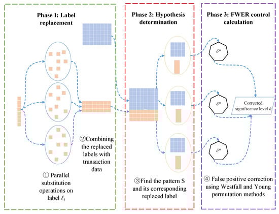
Figure 1. Overall framework of distributed PFWER false positive control.

Since the null hypothesis, $H_0$, proposed in this paper is that pattern S is not significantly associated with label $l_i$, more than one pattern S can be mined in the transactional dataset D. There is a dependency between different patterns, S, and the p-values computed from the labels $l_i$, so the PFWER false positive control is performed using the permutation method proposed by Westfall and Young [30,43]. The permutation-based method is very computationally intensive, so the Spark framework is used for parallel computing to improve the overall computational rate. The algorithm proposed in this chapter can be broadly divided into the following three stages.

• Label permutation operation. According to the replacement method proposed by Westfall and Young [30,43], it is known that to calculate the truncated p-value (corrected significance level $\delta$) more accurately, it is necessary to perform a replacement operation on the label $l_i$ (generally performing $jr={10}^3\sim {10}^4$ times replacement) to achieve the purpose of breaking the association between pattern S and label $l_i$.
• Finding the hypothesis to be tested in multiple hypothesis testing. Since the null hypothesis is composed of two key elements, pattern S and label $l_i$, the main task of the second stage of the algorithm is to find all patterns S and their corresponding labels $l_i$ in the transactional dataset D.
• False-positive correction calculation. After finding the hypotheses to be tested and permuting the labels, the p-value of each hypothesis was calculated according to Fisher’s exact test. The false-positive correction was then performed according to the Westfall and Young [30,43] replacement method, and finally, the FWER was controlled at the $\alpha$ level.

3.3. Index-Tree Algorithm

In order to solve the problem, the hypothesis determination process will dig out a large number of redundant patterns, which affects the computational speed. In this paper, we propose an Index-Tree algorithm, which uses a reduction strategy to reduce the construction of conditional trees and, thus, the computation of patterns. It also adopts an index optimization strategy to reduce the computational overhead caused by multiple traversals of the dataset, further reducing the computation of redundant patterns and speeding up the overall computational speed of the false positive control.

3.3.1. Pattern Mining

The main purpose of pattern mining in this paper is to find all hypotheses. The hypothesis is composed of two key elements patterns S with labels $l_i$, so in the hypothesis determination phase, it is necessary to mine all patterns S by pattern mining methods. Then the hypothesis is determined by traversing the dataset to find the labels that contain the corresponding pattern transactions.

As shown in Figure 2, this paper uses the FP-Growth algorithm for pattern mining. However, since this paper wants to control the false positives in multiple hypothesis testing, that is, to find all patterns S for which the p-value is calculated, the false positive control is performed using the PFWER control method. In other words, the minimum support count in the FP-Growth algorithm is to be set to 1. This makes the computational efficiency of the FP-Growth algorithm for pattern mining very low. Since pattern mining is also only one step in all the computational aspects of this paper, there is a subsequent PFWER false positive control calculation. Therefore, it is necessary to improve the FP-Growth algorithm without changing the effect of the PFWER false positive control in order to reduce the memory overhead and improve the computational efficiency. To solve the above problems, a pruning operation and an index optimization operation are adopted to reduce the redundant patterns and improve the computational efficiency.

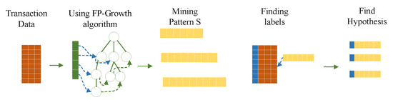
Figure 2. Pattern mining purpose.

3.3.2. Pruning Operation

This chapter focuses on controlling the number of false positive errors in multiple hypothesis testing using the PFWER control method. According to the concept of FWER control, it is known that FWER (family-wise error rate) is the probability of at least one false positive error, and to ensure that the probability of error is as small as possible is to make $FWER\left(\delta \right)\le \alpha$. This means that reducing the significance level of $p_S^F\left(b\right)$ from the original $\alpha$ to $\delta$ is a guarantee that $FWER\left(\delta \right)\le \alpha$. In this way, the problem becomes one of computing the significance threshold $\delta$, where $\delta =max\left\{\delta \right|FWER\left(\delta \right)\le \alpha \}$. Since the Westfall–Young Light algorithm [5] requires $jr={10}^3\sim {10}^4$ times permutation operation for label i in order to make the label unassociated with the pattern, and determines whether a false positive error has occurred by checking whether there is $p_{min}\le \alpha$ where $p_{min}\le min{p}_S^F\left(b\right)$. Then the cluster error rate is calculated as shown in Equation (9).

$$FWER\left(\delta \right)=\frac{1}{jr}\sum _{i=1}^{jr}1[p_{min}^{\left(i\right)}\le \delta ]$$

(9)

where $1\left[p_{min}^{\left(j\right)}\le \delta \right]$ means that if $p_{min}^{\left(j\right)}\le \delta$ is true, then it is 1, otherwise it is 0. The final $\delta$ to be found is the ${\left\{p_{min}^{\left(i\right)}\right\}}_{i=1}^{jr}$ of $\alpha$ quantile point.

Theorem 1.

If there exists $S_1\subseteq S_2$ and $\sigma \left(S_1\right)=\sigma \left(S_2\right)$, then ${\sigma }_1\left(S_1\right)={\sigma }_1\left(S_2\right)$, ${\sigma }_0\left(S_1\right)={\sigma }_0\left(S_2\right)$ and for each permuted label, ${\sigma }_1\left(S_1\right)={\sigma }_1\left(S_2\right)$, ${\sigma }_0\left(S_1\right)={\sigma }_0\left(S_2\right)$.

Theorem 2.

If $S_1\subseteq S_2$ and there exists $\sigma \left(S_1\right)=\sigma \left(S_2\right)$, then $p_{S_1}^F\left(b\right)=p_{S_2}^F\left(b\right)$.

Proof. 

Since $\sigma \left(S_1\right)=\sigma \left(S_2\right)$, the values $\left(n,n_1,\sigma \left(S\right)\right)$ of the edges in the $2\times 2$ column table are fixed, so for $S_1$ and $S_2$, the three values n, $n_1$, and $\sigma \left(S\right)$ are equal. Equations (10) and (11) can be obtained from Equation (7). Obviously, Equation (12) can be derived from Equations (10) and (11). By substituting Equation (12) into the Fisher exact test formula, it can be deduced that $p_{S_1}^F\left(b\right)=p_{S_2}^F\left(b\right)$.

$$p^F({\sigma }_1\left(S_1\right)=a|\sigma \left(S_1\right),n_1,n)=\left(\begin{array}{c}{n}_1\\ a\end{array}\right)\left(\begin{array}{c}n-n_1\\ \sigma \left(S_1\right)-a\end{array}\right)/\left(\begin{array}{c}n\\ \sigma \left(S_1\right)\end{array}\right)$$

(10)

$$p^F({\sigma }_1\left(S_2\right)=a|\sigma \left(S_2\right),n_1,n)=\left(\begin{array}{c}{n}_1\\ a\end{array}\right)\left(\begin{array}{c}n-n_1\\ \sigma \left(S_2\right)-a\end{array}\right)/\left(\begin{array}{c}n\\ \sigma \left(S_2\right)\end{array}\right)$$

(11)

$$p^F({\sigma }_1\left(S_1\right)=a|\sigma \left(S_1\right),n_1,n)=p^F({\sigma }_1\left(S_2\right)=a|\sigma \left(S_2\right),n_1,n)$$

(12)

   □

Theorem 3.

If $S_1\subseteq S_2$ and $\sigma \left(S_1\right)=\sigma \left(S_2\right)$, then only the p-value of mode $S_1$ needs to be computed.

Proof. 

According to Equation (9), it is known that the final estimate of $FWER\left(\delta \right)$ is related to $p_{min}^{\left(i\right)}$ after each permutation and $p_{min}=min{p}_S^F\left(b\right)$. By Theorem 2, we know that if $S_1\subseteq S_2$ and there exists $\sigma \left(S_1\right)=\sigma \left(S_2\right)$, then $p_{S_1}^F\left(b\right)=p_{S_2}^F\left(b\right)$. If $p_{S_1}^F\left(b\right)=p_{S_2}^F\left(b\right)$ is the minimum value of the p-value in this substitution, then $p_{min}$ picks $p_{S_1}^F\left(b\right)$ as the same as the result of $p_{min}$ picking $p_{S_2}^F\left(b\right)$. Therefore, it is sufficient to compute only the p-value $p_{S_2}^F\left(b\right)$ of the mode $S_1$, without computing the p-value of the mode $S_1$. If $p_{S_1}^F\left(b\right)=p_{S_2}^F\left(b\right)$ is not the minimum value of p-value in this replacement, since $p_{S_1}^F\left(b\right)=p_{S_2}^F\left(b\right)$, then $p_{min}$ and $p_{S_1}^F\left(b\right)$ are the same as the result of comparing $p_{S_2}^F\left(b\right)$, so it is sufficient to perform the calculation only once.    □

Theorem 4.

In FP-Tree, if there exists $\sigma \left(I_1\right)=\sigma \left(I_2\right)$ and $I_1.next=I_2$ in the item header table, while for all $I_1.link.next$ and $I_2.link.next$ there are $\sigma \left(I_1.link.next\right)$=$\sigma \left(I_2.link.next\right)$, and in the FP-Tree $I_1.link.next.child=I_2.link.next$ and $I_2.link.next.parent=I_1.link.next$, such that $S_1=S\cup \left\{I_1\right\}$, $S_2=S\cup \left\{I_1,I_2\right\}$, we have $S_1\subseteq S_2$ and $\sigma \left(S_1\right)=\sigma \left(S_2\right)$.

Proof. 

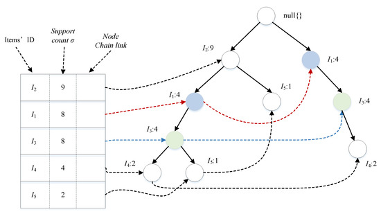
According to {$\left\{I_2,I_5:1\right\}$, $\left\{I_1,I_3:2\right\}$, $\left\{I_1,I_2,I_3:1\right\}$, $\left\{I_1,I_2,I_3,I_5:1\right\}$, $\left\{I_1,I_2,I_3,I_4\right.$$\left.:2\right\}$, $\left\{I_2:4\right\}$, $\left\{I_1,I_3,I_4:2\right\}$} the dataset constructed by the FP-Tree is shown in Figure 3. Where $\sigma \left(I_1\right)=\sigma \left(I_3\right)$, the number of nodes in the item header table is $I_1$ at one position on $I_3$ and for all $I_1$ and $I_3$ chains on the number of supported nodes $\left(\sigma \left(I.link.next\right)\right)$ is the same for all $I_1$ and $I_3$ links. In FP-Tree, all $I_3$ nodes’ parent nodes are $I_1$ nodes and all $I_1$ nodes’ children are $I_3$ nodes. Obviously, there is $\sigma \left(\left\{I_1\right\}\right)=\sigma \left(\{I_1,I_3\}\right)$. Let $S_1=S\cup \left\{I_1\right\}$, $S_2=S\cup \left\{I_1,I_3\right\}$, then $S_1\subseteq S_2$, $\sigma \left(S_1\right)=\sigma (S\cup \left\{I_1\right\})=\sigma \left(S\right)\cap \sigma \left(\left\{I_1\right\}\right)$, $\sigma \left(S_2\right)=\sigma (S\cup \left\{I_1,I_3\right\})=\sigma \left(S\right)\cap \sigma \left(\{I_1,I_3\}\right)$, so $\sigma \left(S_1\right)=\sigma \left(S_2\right)$.    □

Figure 3. Pattern mining purpose.

The nodes $I_1$ and $I_3$ that satisfy the condition of Theorem 4 in the FP-Tree can be combined into one node $I_1$; that is, patterns $S_1$ and $S_2$ can be combined into one pattern, and then according to Theorems 1–3, it is only necessary to calculate the p-value of pattern $S_1$ to reduce the amount of computation in memory and speed up the computation of the single-machine algorithm.

3.3.3. Index Optimization

From the $2\times 2$ column table, we know that after mining pattern S, we need to find all the $S\subseteq T_i$, $l_i=l^1$ support numbers ${\sigma }_1\left(S\right)$, and this process requires traversing the whole dataset once. Since the Westfall–Young Light algorithm [5] starts from a minimum support number of 1, the number of patterns to be mined is very large, and it would be too expensive to traverse the dataset once for each pattern mined to find its ${\sigma }_1\left(S\right)$. When performing pattern mining, an index can be added to speed up the query, which is the position of transaction $T_i$, so that counting $l_i=l^1$ takes only linear time to find. The transaction dataset D with the index added is shown in Table 4.

Table 4. Transaction dataset with index.

Index TID	Labels	Transaction
0	0	$I_2,I_5$
1	1	$I_1,I_3$
2	1	$I_1,I_2,I_3$
3	0	$I_2$
4	0	$I_1,I_2,I_3,I_4$
5	1	$I_1,I_2,I_3,I_4$
6	1	$I_2$
7	1	$I_1,I_3$
8	0	$I_1,I_2,I_3,I_5$
9	0	$I_1,I_3,I_4$
10	1	$I_2$
11	1	$I_2$
12	0	$I_1,I_3,I_4$

The FP-Tree with indexed structure is constructed based on the above dataset, as shown in Figure 4. The conditional pattern bases are constructed on the basis of the indexed FP-Tree, and the conditional pattern bases are constructed from the smallest to the largest support counts, that is, from $I_5:<I_2,I_1:\left\{8\right\}><I_2:\left\{0\right\}>$,$I_4:<I_2,I_1:\left\{3,5\right\}><I_1:\left\{9,12\right\}>$,$I_1:<I_2:\left\{2,3,5,8\right\}>$. Next, we construct the indexed conditional FP-Tree based on the indexed conditional pattern base and find the pattern $SI=\left(\left\{t_i\right\},\left\{TI{D}_i\right\}\right)$ with the index structure. The conditional pattern bases are constructed based on the index FP-Tree by supporting the degree counts from small to large; that is, starting from $I_5:\left\{<I_2,I_1:\left\{8\right\}>,<I_2:\left\{0\right\}>\right\}$,$I_4:\left\{<I_2,I_1:\left\{3,5\right\}><I_1:\left\{9,12\right\}>\right\}$,$I_1:\left\{<I_2:\left\{2,3,5,8\right\}>\right\}$. Next, we construct the indexed conditional FP tree based on the indexed conditional pattern base and find the pattern with the index structure $SI=\left(\left\{t_i\right\},\left\{TI{D}_i\right\}\right)$.

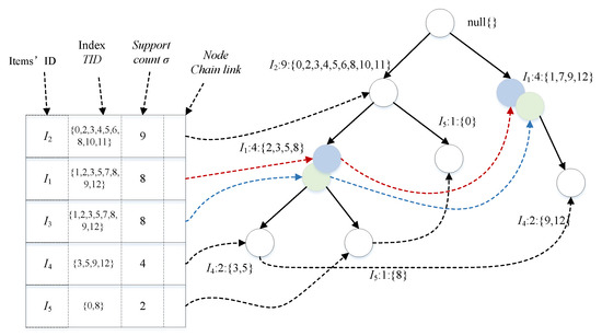
Figure 4. Pattern mining purpose.

The null hypothesis $H_0$ proposed in this paper is that pattern S is not significantly associated with the label $l_i$, and the parameter to be tested in this paper can be set as $\theta =\left\{\left(S,l_i\right)\right|S\subseteq T_j,j=1,\dots ,n,i=0,1\}$. According to Table 3 and Equation (9), the key variables for false positive control for the selected dataset D and the determined null hypothesis $h_0$ are n, $n_1$, $\sigma \left(S\right)$, and ${\sigma }_1\left(S\right)$ in the case of $l_i=l^1$ obtained after label replacement. Where n,$n_1$ can already be determined when the sample dataset is selected, and n,$n_1$ is fixed. While $\sigma \left(S\right)$ and ${\sigma }_1\left(S\right)$ are the support counts when $S\subseteq T_i$ and $l_i=l^1$ and $S\subseteq T_j$, respectively. It is easy to see from the structure of dataset D that once the set of transactions $\left\{T_i\right\}$ to which the pattern S belongs is known, the set of labels $\left\{l_i\right\}$ corresponding to it can be found, and the support count $\sigma \left(S\right)$ is the size of the set $\left\{T_i\right\}$, and it is also not difficult to determine ${\sigma }_1\left(S\right)$ based on the correspondence between transactions and labels. Therefore, it is not necessary to know what the specific pattern S is when performing the PFWER false positive control calculation, but only to know what sets of transactions $\left\{T_i\right\}$ are available to mine the pattern S. Finding out which transaction sets exist that can be mined for patterns is more important for subsequent computation. In this way, it is clearly more advantageous to use a vertical data format for data mining.

The transactional dataset of Table 4 is converted into a vertical data format representation, as shown in Table 5. Data mining is performed to find the patterns to be computed by intersecting the index set of each pair of items in the item set. For example, the index set of the pattern $\left\{I_1,I_2\right\}$ is $TID\left(I_1,I_2\right)=TID\left(I_1\right)\cap TID\left(I_2\right)=\left\{2,3,5,8\right\}$.

Table 5. Vertical data format transaction dataset.

Item Set	TID-Set
$I_1$	$\left\{1,2,3,5,7,8,9,12\right\}$
$I_2$	$\left\{0,2,3,4,5,6,8,10,11\right\}$
$I_3$	$\left\{1,2,3,5,7,8,9,12\right\}$
$I_4$	$\left\{3,5,9,12\right\}$
$I_5$	$\left\{0,8\right\}$

Theorem 5.

If there exists $TID\left(S_1\right)=TID\left(S_2\right)$, then $p_{S_1}^F\left(b\right)=p_{S_2}^F\left(b\right)$.

Proof. 

If there exists $TID\left(S_1\right)=TID\left(S_2\right)$, then it means that the number of transactions containing patterns $S_1$ and $S_2$ are equal, i.e., $\left|TID\left(S_1\right)\right|=\left|TID\left(S_2\right)\right|$, so there is $\sigma \left(S_1\right)=\sigma \left(S_2\right)$. Again, since labels have a one-to-one correspondence with transactions, although $jr$permutations are performed, pattern $s_1$ belongs to the same transaction set as pattern $s_2$. Therefore, for each permutation, there is ${\sigma }_1\left(S_1\right)={\sigma }_1\left(S_2\right)$. The total number of transactions n is fixed with the number of labels $l_i=l^1$ for the same dataset $n_1$, substituting $\sigma \left(S\right)$, ${\sigma }_1\left(S\right)$, n and $n_1$ into Equations (7) and  (8) to find $p_{S_1}^F\left(b\right)=p_{S_2}^F\left(b\right)$.    □

Substituting $p_{S_1}^F\left(b\right)=p_{S_2}^F\left(b\right)$ into Equation (9) (FWER false positive control formula) shows that $p_{S_1}^F\left(b\right)$ has the same effect as $p_{S_2}^F\left(b\right)$ on Equation (9), so their calculated p-values have the same influence on Equation (9) for different patterns with the same index set, so it is sufficient to perform the p-value calculation only once.

Based on the above problem analysis, it is clear that mining the set of transactions containing pattern S is more useful for the subsequent computation than mining all patterns in the dataset and then computing the corresponding dataset. Inspired by the vertical data format, the index tree is pruned again according to Theorem 5 to reduce the computation of invalid patterns generated in the data mining process.

The conditional pattern base of $I_4$ is $<I_2,I_1:\left\{3,5\right\}><I_1:\left\{9,12\right\}>$ according to the item header table in Figure 4, and the conditional tree constructed from this conditional pattern base is shown in Figure 5. The conditional tree using $I_4$ is pattern mined using the FP-Growth algorithm by combining all nodes on this single path and then combining the combined set with that node to form the pattern output. According to the above statement, from the conditional tree of $I_4$, we will receive $S_1=\left\{I_1,I_4,\left\{3,5,9,12\right\}\right\}$, $S_2=\left\{I_2,I_4,\left\{3,5\right\}\right\}$, $S_3=\left\{I_1,I_2,I_4,\left\{3,5\right\}\right\}$, but actually patterns $S_2$ and $S_3$ are exactly equal for the PFWER false positive control calculation, and there is no need to repeat the calculation; therefore, it is only necessary to know the index set of each node to substitute into the FWER control formula for the calculation. When the number of nodes contained in a single-path conditional tree is very large, it can reduce a lot of additional computational overhead.

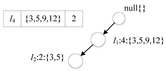
Figure 5. Condition tree of $I_4$.

The purpose of Algorithm 1 is to mine the index set containing the patterns and to provide computational preparation for the subsequent PFWER false positive control. The first line of the algorithm constructs the set of frequent1 -items and calculates their support counts. The second line of the algorithm constructs the index tree. In the third line of the algorithm, it calls Algorithm 2 to perform pruning operations on the index tree. If the condition tree contains only a single path, then the index set of nodes on this path is output, otherwise, the condition tree is constructed for the pattern $\beta \cup \alpha$ in the tenth to thirteenth lines of the algorithm, and if the condition tree is not controlled, then the algorithm is recursively called for mining, and finally, all index sets containing the pattern are obtained.

The first line of Algorithm 2 iterates through the nodes in the item head table, and the second to fifth lines determine whether two adjacent nodes with the same support count in the item head table are to be merged. If the nodes in the FP tree satisfy the pruning condition in Section 3.3.2, the nodes in the FP tree are merged in the sixth line of the algorithm, the term header table is updated, and the pruned index tree is returned.

Algorithm 1 Index Tree

Require:   $D=\left\{\left(T_i,l_i\right)\right\}$ Ensure:  $In=\left\{TI{D}_i\right\}$  1: $create\left(item\_1\right),\sigma \leftarrow size\left(index\right)$  2: $IFP\_Tree\leftarrow createTree(item\_1,D)$  3: $tree\leftarrow IPFP\_Tree(IFP\_Tree)$  4: $IFP\_Growth(tree,\beta )$  5: if  $path\in tree$ then  6:    for $node\in path$ do  7:        $TID(\beta \cup node)$  8:    end for  9: else 10:    for each $a_i\in (a_i,TI{D}_b)$ do 11:        $b\leftarrow \beta \cup a_i$$TI{D}_b\leftarrow TI{D}_a$$\sigma \leftarrow size\left(TI{D}_b\right)$ 12:        $create\left(D_b\right)$ 13:        $create\left(tre{e}_b\right)$ 14:        $tre{e}_{ib}\leftarrow IPFP-Tree\left(tre{e}_b\right)$ 15:        if $tre{e}_{ib}\ne ⌀$ then 16:           $IFP-Growth(tre{e}_{ib},b)$ 17:        end if 18:    end for 19: end if

Algorithm 2 IPFP Tree

Require:  $items$ Ensure:  $IPFP-tree$  1: for  $i\in items$  do  2:     if $\sigma Head\left(i\right))=\sigma Head(i-1\left)\right)$ then  3:         for $nod{e}_i\in lin{k}_i$, $nod{e}_{i-1}\in lin{k}_{i-1}$ do  4:             if $\sigma \left(nod{e}_i\right)=\sigma \left(nod{e}_{i-1}\right)$ then  5:                 if $nod{e}_i.child=nod{e}_{i-1}$ and $nod{e}_{i-1}.parent=nod{e}_i$ then  6:                     $remove\left(nod{e}_{i-1}\right)$  7:                     $update\left(Head\right)$  8:                 end if  9:             end if 10:        end for 11:     end if 12:     $i\leftarrow i+1$ 13: end for

3.4. Distributed PFWER Control Algorithm

3.4.1. Label Replacement

The first stage of the distributed PFWER false positive control algorithm is the label replacement stage, where the purpose of label replacement is to make no relationship between labels and patterns. Therefore, it is necessary to disrupt and reshuffle the labels, which generally requires $jr={10}^3\sim {10}^4$ times the permutation of the labels. This process can be run in parallel on the cluster, and the execution is shown in Figure 6.

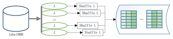
Figure 6. Parallel label replacement.

First, we read the label data using the sc.textFile() method and store it in labelRDD; then we perform a random permutation operation on the read labels in parallel. Then we perform a merge operation on the disordered set of labels in the cluster, and finally, we receive a permuted set of labels.

3.4.2. Hypothesis Determination

The second part of the distributed PFWER false positive control algorithm is to find the parameters to be tested in the multiple hypothesis test. Since the null hypothesis is composed of two key elements, pattern S and label $l_i$, it is known from the theorem in Section 3.3 that the parameters to be determined in the actual computation are the set of all indexes mapped to pattern S and their corresponding labels $l_i$ in the transaction dataset D, so the main task in this stage is to find the above two parameters.

Based on the PFWER false positive control characteristics combined with the Index-Tree algorithm in Section 3.3, this leads to a distributed computational method for hypothesis determination and the parallel computation of index sets and their labels mapped to patterns. The method consists of three important phases divided into a dataset-partitioning phase, a frequent 1-item set and FP tree construction phase, and a group mining phase with pattern-mapped index sets and their labels. Figure 7 shows the computational framework of distributed hypothesis determination, where the dataset is divided into n partitions in the dataset partitioning phase and subsequent computations are performed in parallel. The main objective of the frequent 1-item set and FP tree construction phase is to construct frequent 1-item sets with index structures and to construct FP trees with index structures based on frequent 1-item sets and transactional datasets. Figure 8 illustrates the process of constructing a frequent 1-term set as follows

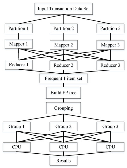
Figure 7. Find hypothetical computing frameworks in parallel.

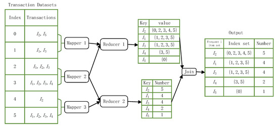
Figure 8. Constructing frequent 1-item sets.

• First, the items in the dataset should be split using the flatMap operator to construct <key = item,value = index> key-value pairs in parallel and the map operator to construct <key = item,value = 1> key-value pairs.
• Secondly, the key-value pairs of <key = item,value = 1> are computed cumulatively using the reduceByKey algorithm. The computed key is the item name, and the value is the number of items in the dataset.
• Next, the key-value pair <key=item,value = index> is computed using the groupByKey operator to obtain a new key-value pair <key = item,value = index>, where the value is the index set containing the key values.
• Finally, use the join operator to combine <key = item,value = index> and <key = item,value = count> into a new key-value pair <key = item,value = count + index> and output it in descending order of the count of the values in each key-value pair to get the item header table for subsequent calculations.

The FP tree with index structure is constructed by traversing the transaction dataset based on the frequent 1-item sets with index structure. Next, the frequent 1-item set is divided into h groups, the group numbers are denoted by $hid$, and each group contains a complete FP tree with an index structure. The conditional pattern base and the conditional pattern tree are constructed for each $hid$ group, and then the index set containing the patterns is mined using the Index-Tree algorithm. Since the labels correspond to the transaction data, the index set containing the patterns can be computed while the corresponding label set can be determined, and obviously, the two parameters related to the null hypothesis in the hypothesis test have been determined.

3.4.3. False Positive Control

This section mainly uses the false positive control method proposed by Westfall and Young [30,43] to control the FWER at the $\alpha$ level, which is implemented with the main idea that a new resampled transactional dataset with no relationship between patterns and labels can be generated by just randomly arranging the class labels. This allows one to determine whether a false positive error has occurred by computing the minimum p-value after each permutation, $p_{min}=min{p}_S^F$, and checking whether $p_{min}\le \delta$ holds. The subsequent sections of this paper refer to this method as the WY replacement algorithm.

The disadvantage of the WY replacement algorithm is that it is computationally expensive in addition to having a large number of replacement operations. Terada [13] and other researchers found that in Fisher’s exact test, when $2\times 2$ columns are fixed, then the value $\left(n,n_1,\sigma \left(S\right)\right)$ at the edge of the table is also fixed, and according to Equations (7) and (8) it is not difficult to find that the p-value is ultimately a function about ${\sigma }_1\left(S\right)$. Since the objects in the $2\times 2$ column table are discrete and can only take finitely many values, it can be determined that ${\sigma }_1\left(S\right)$ is bounded, i.e., ${\sigma }_1\left(S\right)\in \left[{\sigma }_1{\left(S\right)}_{min},{\sigma }_1{\left(S\right)}_{max}\right]$. Where ${\sigma }_1{\left(S\right)}_{max}=min\left(n_1,\sigma \left(S\right)\right)$, ${\sigma }_1{\left(S\right)}_{min}=max\left(0,\sigma \left(S\right)-\left(n-n_1\right)\right)$. From the bound of ${\sigma }_1\left(S\right)$, it can also be further deduced that there exists a minimum reachable p-value $\phi \left({\sigma }_S\right)$ strictly greater than 0 as follows.

$$\phi ({\sigma }_S)=min\left\{p_S^F\left(a\right)\right|{\sigma }_1{\left(S\right)}_{min}\le a\le {\sigma }_1{\left(S\right)}_{max}\}$$

(13)

According to Equation (8), the p-value calculated for Fisher’s exact test is the cumulative sum of the results obtained using Equation (7), and the values calculated in Equation (7) are all greater than 0. It can be inferred that when ${\sigma }_1\left(S\right)={\sigma }_1{\left(S\right)}_{min}$ or ${\sigma }_1\left(S\right)={\sigma }_1{\left(S\right)}_{max}$, the minimum reachable p-value $\phi \left({\sigma }_S\right)$. It is then possible to call all patterns S of $\phi \left({\sigma }_S\right)\le \delta$ the set of measurable patterns so that patterns not in the set of $\kappa \left(\delta \right)$ cannot be statistically significant under $\delta$. On this basis, a monotonically decreasing lower bound $\widehat{\phi }\left(\sigma \right)$ on the minimum achievable p-value can be introduced, as shown in Equation (14).

$$\widehat{\phi }\left(\sigma \right)=\left\{\begin{array}{cc}\phi \left({\sigma }_S\right)& 0\le {\sigma }_S\le n_1\\ 1/\left(\begin{array}{c}n\\ n_1\end{array}\right)& n_1\le {\sigma }_S\le n\end{array}\right.$$

(14)

The monotonically decreasing lower bound $\widehat{\phi }\left(\sigma \right)$ on the minimum achievable p-value gives $\widehat{\kappa }\left(\delta \right)=\left\{S|\widehat{\phi }\left(\sigma \right)\le \delta \right\}$, which satisfies $\kappa \left(\delta \right)\subset \widehat{\kappa }\left(\delta \right)$, which, in turn, can be rewritten as $\widehat{\kappa }\left(\delta \right)=\left\{S|{\sigma }_S\ge {\sigma }_{\delta }\right\}$ due to monotonicity. That means only the mode S satisfying condition $\widehat{\kappa }\left(\delta \right)=\left\{S|{\sigma }_S\ge {\sigma }_{\delta }\right\}$ is valuable for the PFWER false positive control calculation. Based on the above, the pseudo-code of the distributed PFWER false positive control algorithm is proposed, as shown in Algorithms 3 and 4.

Algorithm 3  DS-FWER(D)

Require:  D Ensure:  $\delta$  1:  $label\leftarrow DistributedLabelPermutation\left(D\right)$  2:  $p_{min}^{\left(i\right)}\leftarrow 1$  3:  $\sigma \leftarrow 1$, $\delta \leftarrow \widehat{\phi }\sigma$  4:  $itemIndex\leftarrow flatMap\left(D\right)$, $itemOne\leftarrow map\left(D\right)$  5:  $itemCount\leftarrow reduceByKey\left(itemOne\right)$, $itemIndexs\leftarrow groupByKey\left(itemInedx\right)$  6:  $item\leftarrow itemCount.join\left(itemIndexs\right)$  7:  $tree\leftarrow createF1Tree\left(item\right)$, $F1\_tree\leftarrow IPFP-Tree\left(tree\right)$  8:  $itemGroup\leftarrow group\left(item\right)$  9:  $index\leftarrow Index-tree(itemGroup,F1\_tree)$ 10:  $WY(index,label)$ 11:  Return $\alpha$ quantile of ${\left\{p_{min}^{\left(i\right)}\right\}}_{i=1}^{jr}$

Algorithm 4 WY Algorithm

Require:  $index,label$ Ensure:  $\sigma$  1:  $p_S^F\left({\sigma }_1\left(S\right)\right)$  2:  for  $i=1,\dots ,jr$  do  3:      Compute ${\sigma }_1\left(S\right)$  4:      $p_{min}^{\left(i\right)}\leftarrow \left\{p_{min}^{\left(i\right)},p_S^F\left({\sigma }_1\left(S\right)\right)\right\}$  5: end for  6: $FWER\left(\delta \right)=\frac{1}{jr}{\sum }_{i=1}^{jr}1\left[p_{min}^{\left(i\right)}\le \delta \right]$  7: while  $FWER\left(\delta \right)>\alpha$do  8:      $\sigma \leftarrow \sigma +1$$\delta \leftarrow \widehat{\phi }\left(\sigma \right)$  9:      $FWER\left(\delta \right)=\frac{1}{jr}{\sum }_{i=1}^{jr}1\left[p_{min}^{\left(i\right)}\le \delta \right]$ 10: end while 11: for  $inde{x}^{\prime }\in List\left\{index\right\}$do 12:      Compute $\sigma \left(S\right)$ 13:      if $\sigma \left(S\right)\ge \sigma$ then 14:          $WY(inde{x}^{\prime },label)$ 15:      end if 16: end for

The first line of Algorithm 3 uses distributed label permutation to obtain the permuted label set with indexed positions, the second line initializes all minimum p-values in $jr$ permutation calculations to 1, the third line initializes the minimum support of the pattern, and the modified significance threshold $\delta$ is initialized according to this minimum support for subsequent calculations. The fourth to seventh lines of the algorithm uses parallel methods to construct frequent 1-item sets with indexed structures with FP trees, and the eighth line groups the frequent 1-item sets and distributes the grouped data to each node in the cluster. We rewrite the Index-Tree algorithm and change its input to FP tree and frequent 1-item sets, and mine its index set on each node according to FP tree and the grouped frequent 1-item sets. Finally, the index set and label set are substituted into the WY replacement algorithm to obtain the set of $jr$ minimum p-values ${\left\{p_{min}^{\left(i\right)}\right\}}_{i=1}^{jr}$, then the significance threshold of p-value calculation is set to ${\left\{p_{min}^{\left(i\right)}\right\}}_{i=1}^{jr}$ of the $\alpha$ quantile will eventually control the FWER under the $\alpha$ level.

Algorithm 4 is the WY permutation algorithm. The first line of the algorithm computes all p-values $p_S^F\left({\sigma }_1\left(S\right)\right)$ in the bounds using Fisher’s exact test. The second to fourth lines of the algorithm calculate the ${\sigma }_1\left(S\right)$ value of the index set for each permutation for $jr$ permutations and calculate the minimum p-value $p_{min}^{\left(i\right)}$. The fifth line of the algorithm finds the current $FWER\left(\delta \right)$ value based on ${\left\{p_{min}^{\left(i\right)}\right\}}_{i=1}^{jr}$. Lines six to eight of the algorithm perform a round-robin operation where the minimum support is the current minimum support plus 1 if $FWER\left(\delta \right)>\alpha$ and update the significance threshold at the same time until $FWER\left(\delta \right)\le \alpha$. For all the mined index sets of $\sigma \left(S\right)\ge \sigma$, the WY replacement algorithm is executed to find the final modified significance threshold. Finally, the corrected significance thresholds found on each node are compared, and the smallest significance threshold among all nodes is the final result.

3.5. Proof of Correctness

The first is the correctness of the data cut, and the second is the correctness of the final result obtained by executing the WY permutation algorithm in parallel.

According to Section 3.3, we can find the index sets of all patterns S and perform the de-duplication operation on these index sets before performing the PFWER false positive control computation to reduce the amount of data to be computed while ensuring the correctness of the result computation. This chapter uses the distributed false positive control algorithm process to group the frequent 1-item sets with index structure, and each node will use the index FP tree and the grouped frequent 1-item sets for index set mining. The Index-Tree algorithm determines the conditional pattern base for each item in the head table based on the FP tree and then constructs a conditional tree based on the conditional pattern base to perform subsequent pattern mining. Therefore, as long as the initial index FP tree is consistent for each set of item headers, the index set obtained by the distributed computation will be the same as the index set obtained in the stand-alone case.

Theorem 6.

The minimum value of the significance threshold among all nodes is the overall significance threshold, and the overall significance threshold is the same as the result of the significance threshold computed by a single machine.

Proof. 

The WY replacement algorithm for example performs $\sigma =\sigma +1$ and $\delta =\widehat{\phi }\left(\sigma \right)$ operations whenever it meets $FWER\left(\delta \right)>\alpha$. Let $I{n}_1$ and $I{n}_2$ be two different index sets at different nodes with $I{n}_1$ and $I{n}_2$ support of ${\sigma }_{I{n}_1}$ and ${\sigma }_{I{n}_2}$, and ${\sigma }_{I{n}_1}<{\sigma }_{I{n}_2}$. According to Equation (9) and ${\delta }^{\prime }=max\left\{\delta \left|FWER\right(\delta \le \alpha )\right\}$ we can find ${\delta }_{I{n}_2}^{{}^{\prime }}<{\delta }_{I{n}_1}^{{}^{\prime }}$, which also verifies the property that $\delta$ decreases monotonically with $\sigma$. Therefore, $I{n}_2$ index sets smaller than the current support count can be directly ignored and will not have an impact on the final result, so the final significance threshold is the minimum of the significance thresholds obtained for all nodes and is the same as the result of the stand-alone calculation. □

4. Experiments and Performance Analysis

This chapter validates the algorithm through experiments in the following four areas: Section 4.3.1 determines the parameters used in the distributed PFWER false positive control. Section 4.3.2 tests the pruning efficiency of the algorithm and verifies the effect of the pruning operation on the algorithm. Section 4.3.3 focuses on verifying the accuracy of the calculation of the distributed PFWER false positive control algorithm. Section 4.3.4 tests the operational efficiency of the distributed PFWER false positive control algorithm by comparing the runtime of the distributed PFWER false positive control algorithm with that of the stand-alone PFWER false positive control algorithm using different datasets. The above four experimental directions verify the difference between the distributed false positive control algorithm and the stand-alone false positive control algorithm for false positive control results on the one hand. On the other hand, the distributed false positive algorithm is verified for its ability to improve the computation rate. The experiments use different datasets to demonstrate the robustness and general applicability of the algorithms.

4.1. Experimental Environment Configuration

The algorithm in this paper is written in Java language and uses the Spark framework for distributed computation. The experimental code writing environment is shown in Table 6.

Table 6. Coding environment description.

Encoding Software and Hardware Environment
CPU	Intel(R) Core(TM) i7-10750H CPU @ 2.60 GHz 2.59 GHz
Memory	16.00 GB
Hard disk	500 GB
Operating System	Windows 10
System type	64-bit OS, x64-based processor
Development tools	IEDA
Development environment	JDK1.8, Hadoop2.7.7, Spark2.4.4

The algorithm proposed in this paper is a distributed false positive control algorithm, so the main experimental part of the algorithm is completed on the cluster. The test cluster environment of the experiment is shown in Table 7.

Table 7. Experimental environment description.

Test Software and Hardware Environment
CPU	Intel(R) Xeon(R) CPU E5-2420 0 @ 1.90 GHz
Memory	24.00 GB
Hard disk	2TB
Operating system	Red Hat Enterprise Linux Server release 6.3
System type	X86_64
Experimental environment	JDK1.8,Hadoop2.7.7,Spark2.4.4

4.2. Experimental Dataset

The information on the datasets used in the experiments of this paper is shown in Table 8. We performed our experiments using 11 datasets: they are available at FIMI’04 (http://fimi.ua.ac.be, 7 June 2022), UCI (https://archive.ics.uci.edu/ml/index.php, 7 June 2022) and kdd2018 (https://github.com/VandinLab/TopKWY, 10 June 2022). The datasets labeled with (L) in the dataset description are the datasets with binary classification labels, and the datasets labeled with (U) are the datasets without classification. For datasets without transactions classified into two categories, a single item with a frequency closer to 0.5 is chosen to be removed from the transaction dataset to artificially divide the dataset into two groups, and $n/n_1$ is used to represent the ratio of the number of transactions in the dataset to the number of transactions labeled $l^1$, with two decimal places retained.

Table 8. Experimental dataset.

Dataset	|D|	Number of Items	Average Length of Transactions	$\mathit{n}/{\mathit{n}}_1$
Mushroom(L)	8124	118	22	2.08
Breast Cancer(L)	7325	1129	6.7	11.11
A9a(L)	32,561	247	13.9	4.17
Bms-Web1(U)	58,136	60,978	2.51	33.33
Bms-Web2(U)	77,158	330,285	4.59	25
Retail(U)	88,162	16,470	10.3	2.13
Ijcnn1(L)	91,701	44	13	10
T10I4D100K_new(U)	100,000	870	10.1	12.5
Codrna(L)	271,617	16	8	3.03
Covtype(L)	581,012	64	11.9	2.04
Susy(U)	5,000,000	190	43	2.08

4.3. Distributed PFWER False Positive Control Experiment

4.3.1. Determination of The Number of Permutations

• Experimental description: This section focuses on determining the parameter used in the distributed PFWER false positive control, i.e., the number of label replacements, jr. Label replacement is an important element to ensure the accuracy of the distributed PFWER false positive control results, and its purpose is to make sure there is no relationship between labels and patterns. The null hypothesis proposed in this paper is satisfied by the absence of an association between the mode and label and by avoiding the influence of inter-mode dependencies on the computational results. The experiment is to test the effect of the PFWER false positive control algorithm on the false positive control effect by setting different numbers of substitutions in the label substitution stage. In this paper, the FP-Growth algorithm will be used to perform the pattern mining operation for all comparison experiments.
• Experimental analysis: The distributed PFWER false positive control uses a permutation-based approach for the control calculation. The known cost in setting the permutation value, jr, is that the larger the jr, the more accurate the final corrected significance threshold is estimated, but the cost is that the running time increases with the increase in jr. The following figure represents the computation for different datasets with different jr.

The horizontal coordinate of Figure 9 is the number of permutations, jr, and the vertical coordinate indicates the final support count. Figure 10 indicates the running time corresponding to different datasets selected with different replacement counts, the horizontal coordinate is the replacement count jr, and the vertical coordinate indicates the running time in (s). Since the label replacement is a random replacement process, there will be individual label disruptions that are not very good in the process of disrupting the label order. However, from the overall experimental results, the support count tends to be stable at $jr={10}^3\sim {10}^4$; if the number of permutations is increased on this basis, it has little effect on the calculation but will greatly increase the running time of the algorithm, so the experimental parameter chosen in this paper is $jr={10}^3$ or $jr={10}^4$.

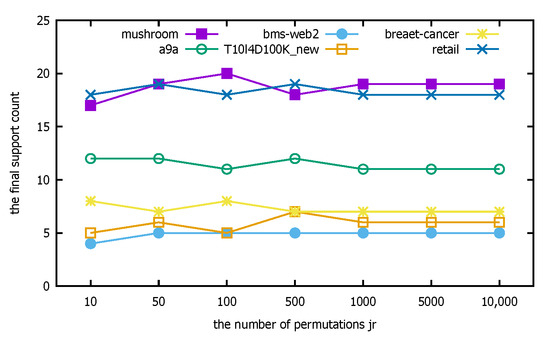
Figure 9. The number of replacement experiments.

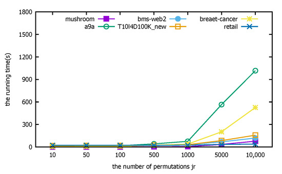
Figure 10. Run time changes.

4.3.2. Pruning Efficiency Analysis

(1)

Experimental description

The PFWER false positive control algorithm needs to find all the hypotheses to be tested in the dataset, and these hypotheses to be tested are composed of the patterns mined in the transaction set and their corresponding permuted labels. Therefore, it is necessary to use techniques related to pattern mining. In the computation process, it is found that using Fisher’s exact test to calculate the p-value and using the WY replacement process for false positive control can reduce the computation of PFWER false positive control by some pruning operations and speeding up the computation, which does not affect the computation results.

The purpose of the experimental tests in this section is to verify the effect of pruning operations on the algorithm. From the above experimental description, it can be seen that the execution of the pruning operation reduces the number of patterns to be calculated for PFWER false positive control and does not affect the false positive control effect. Therefore, the experiments in this section will verify the efficiency of the pruning operation in terms of both the number of patterns that need to be computed before and after the pruning operation and the change in the significance threshold.

(2)

Experimental analysis

The purple bars in Figure 11 show the number of patterns mined before the pruning operation, and the green bars show the number of patterns mined after the pruning operation. The experimental results show that the use of the pruning operation in the calculation of the PFWER false positive control can effectively reduce the number of patterns calculated, thus reducing the number of p-values that need to be calculated by Fisher’s exact test and thus can effectively improve the efficiency of the PFWER false positive control.

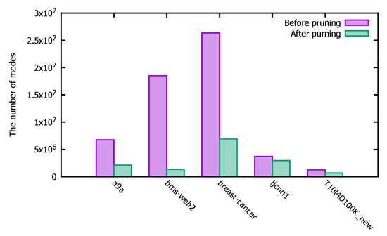
Figure 11. The number of modes before and after pruning operations in different datasets.

Table 9 shows the effect of pruning on the run speed of different datasets before and after the pruning operation, and it can be seen from the data in the table that for most of the datasets, the pruning operation can improve the run efficiency.

Table 9. Time comparison before and after pruning.

Dataset	Mushroom	A9a	Bms-Web2	Breast Cancer	Cod-Rna	Retail	Ijcnn1
Before pruning (s)	656.3	1706.9	226.0	833.9	1066.3	53.4	8837.0
After pruning (s)	77.5	1016.5	119.25	526.3	844.2	39.5	7157.1

Figure 12 represents the changes in the support counts of different datasets before and after the pruning operation. From the experimental results in Figure 12, we can see that the results calculated by the PFWER false positive control algorithm before and after performing the pruning operation are basically the same, thus verifying the correctness of the pruning operation.

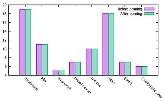
Figure 12. Impact of pruning operation on support count.

Figure 13 shows the comparison of the significance thresholds of the PFWER false positive control after performing pruning operations with and without the pruning operation on different datasets, with the vertical coordinate as the logarithm with base 10. Since the PFWER false positive control performs random permutations of jr times labels that affect the final significance threshold results, it is acceptable to have some deviation in the significance thresholds after performing the pruning operation with and without pruning on individual datasets.

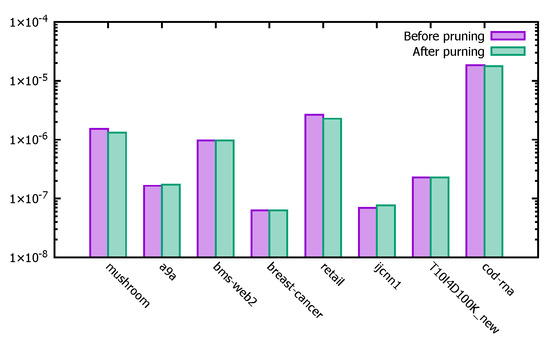
Figure 13. Significant threshold before and after pruning operation.

4.3.3. Accuracy Test

(1)

Experiment Description

The experiments in this section focus on verifying the accuracy of the computation of the distributed PFWER false positive control algorithm. The distributed PFWER false positive algorithm will process the data in the transaction dataset and then perform the PFWER false positive control calculation in parallel on each node of the cluster. The most important point in this process is to ensure that the calculation results of the algorithm in the distributed case are consistent with the results of the stand-alone calculation. The most important point in this process is to ensure that the algorithm’s computational results in the distributed case are consistent with those of the stand-alone computation. The main reason for ensuring the same results of the two runs is that the corrected saliency thresholds obtained in the end are the same.

(2)

Experimental Analysis

Figure 14 gives a comparison of the minimum support calculated by the distributed PFWER false positive control with that of the stand-alone PFWER false positive control, from which it can be seen that the final minimum support obtained for different datasets performing PFWER false positive control is basically the same in the distributed and stand-alone cases, demonstrating the accuracy of the distributed algorithm calculation.

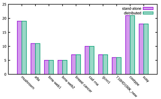
Figure 14. PFWER support for different datasets.

Figure 15 shows the final corrected significant threshold for the distributed PFWER false positive control versus the corrected significant threshold obtained from the PFWER false positive control in the stand-alone case, with the vertical coordinate as the logarithm with base 10. The experimental results show that the results of the corrected significance thresholds obtained for the single machine on different datasets are in general agreement with the results calculated by the distributed PFWER false positive control algorithm proposed in this paper.

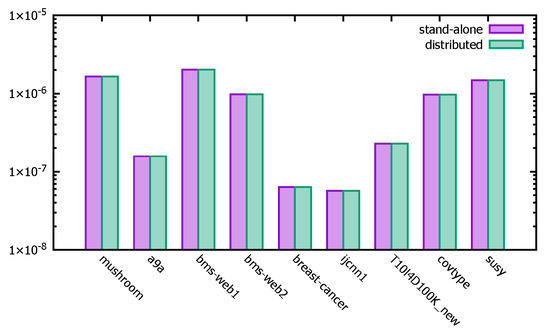
Figure 15. Modified significance thresholds for different datasets of PFWER.

4.3.4. Operational Efficiency Test

(1)

Experimental Description

The main purpose of using distributed techniques for PFWER false positive control calculations in this paper is to improve the computational efficiency of the procedure. The distributed PFWER false-positive control algorithm reduces the time spent on the experiment and does not affect the final results of the experiment, as the model is reduced in the hypothesis determination. In this section, the runtime of the distributed PFWER false positive control algorithm, the stand-alone PFWER false positive algorithm, and the existing FastWY [13] and WYlight [5] algorithms are compared using different datasets to test the efficiency of the distributed PFWER false positive control algorithm.

(2)

Experimental Analysis

The running time units for the algorithms in Figure 16 are seconds (s). The experiments focus on showing a comparison of the run times of the distributed PFWER false positive control algorithm, the stand-alone PFWER false positive algorithm, the FastWY algorithm [13], and the WYlight algorithm [5] running different datasets. The experimental results show that the use of the distributed PFWER false positive control algorithm can effectively improve the computational speed of the algorithm while avoiding the limitations of the stand-alone in-memory computation and can efficiently perform false positive control computations in large-scale data situations, which is of good use.

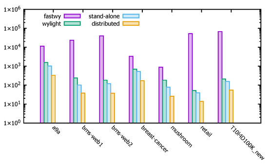
Figure 16. Runtime comparison of distributed PFWER control algorithms with existing algorithms.

4.4. Summary

The distributed PFWER false positive control algorithm has been analyzed and tested experimentally. The experimental data show that the distributed PFWER false positive control algorithm has the same control results as the stand-alone case and is better in terms of operational efficiency than running on a single machine. The algorithm can effectively address the problem of excessive computation in multiple hypothesis testing of false positive control for large data.

5. Conclusions

The PFWER control algorithm can obtain a single hypothesis-test significance threshold subject to an arbitrarily specified overall false positive level constraint without assuming an independent identical distribution. Since the PFWER control algorithm is highly time-consuming, this paper proposes a distributed solution to the PFWER control algorithm, which significantly improves the execution efficiency of the PFWER control algorithm without any loss in theoretical accuracy. Specifically, we abstract the PFWER control problem as a frequent pattern mining problem, and by adapting the FP growth algorithm and introducing distributed computing techniques, the constructed FP tree is decomposed into a set of subtrees, each corresponding to a subtask. All subtrees (subtasks) are distributed to different computing nodes, and each node independently computes the local significance threshold according to the assigned subtasks. The local computation outcomes from every node are aggregated, and the FWER false positive control thresholds are calculated to be exactly in line with the theoretical outcomes. To the best of our knowledge, this is the first paper to present a distributed PFWER control algorithm. Experimental results on real datasets show that the proposed algorithm is more computationally efficient than the comparison algorithm.

In the future, we may also consider using unconditional exact tests, i.e., Barnard’s exact tests, to calculate p-values in false positive control methods for multiple hypothesis testing. Unconditional tests, on the other hand, are generally more expensive than conditional tests (often Fisher’s exact tests) because unconditional tests take into account the various scenarios observed in the pattern frequencies and the actual dataset and require the use of an unknown perturbation parameter for subsequent calculations. Another possible path is to extend this paper’s distributed algorithm to multi-categorically labeled transactional datasets, and to explore efficient distributed control of false positives in multiple hypothesis testing processes in other types of datasets.

References

- Erdogmus, H. Bayesian Hypothesis Testing Illustrated: An Introduction for Software Engineering Researchers. ACM Comput. Surv. 2023, 55, 119:1–119:28. [Google Scholar] [CrossRef]
- Munoz, A.; Martos, G.; Gonzalez, J. Level Sets Semimetrics for Probability Measures with Applications in Hypothesis Testing. Methodol. Comput. Appl. Probab. 2023, 25, 21. [Google Scholar] [CrossRef]
- Li, Y.; Zhang, C.; Shelby, L.; Huan, T.C. Customers’ self-image congruity and brand preference: A moderated mediation model of self-brand connection and self-motivation. J. Prod. Brand Manag. 2022, 31, 798–807. [Google Scholar] [CrossRef]
- Jensen, R.I.T.; Iosifidis, A. Qualifying and raising anti-money laundering alarms with deep learning. Expert Syst. Appl. 2023, 214, 119037. [Google Scholar] [CrossRef]
- Llinares-López, F.; Sugiyama, M.; Papaxanthos, L.; Borgwardt, K.M. Fast and Memory-Efficient Significant Pattern Mining via Permutation Testing. In Proceedings of the 21th ACM SIGKDD International Conference on Knowledge Discovery and Data Mining, Sydney, NSW, Australia, 10–13 August 2015; Cao, L., Zhang, C., Joachims, T., Webb, G.I., Margineantu, D.D., Williams, G., Eds.; ACM: New York, NY, USA, 2015; pp. 725–734. [Google Scholar] [CrossRef]
- Dey, M.; Bhandari, S.K. FWER goes to zero for correlated normal. Stat. Probab. Lett. 2023, 193, 109700. [Google Scholar] [CrossRef]
- Samarskiĭ, A. Claverie JM: The significance of digital gene expression profiles. Genome Res. 1997, 7, 986–995. [Google Scholar]
- Holm, S. A simple sequentially rejective multiple test procedure. Scand. J. Stat. 1979, 6, 65–70. [Google Scholar]
- Simes, R.J. An improved Bonferroni procedure for multiple tests of significance. Biometrika 1986, 73, 751–754. [Google Scholar] [CrossRef]
- Hochberg, Y. A sharper Bonferroni procedure for multiple tests of significance. Biometrika 1988, 75, 800–802. [Google Scholar] [CrossRef]
- Pellegrina, L.; Vandin, F. Efficient Mining of the Most Significant Patterns with Permutation Testing. In Proceedings of the 24th ACM SIGKDD International Conference on Knowledge Discovery & Data Mining (KDD 2018), London, UK, 19–23 August 2018; Guo, Y., Farooq, F., Eds.; ACM: New York, NY, USA, 2018; pp. 2070–2079. [Google Scholar] [CrossRef]
- Hang, D.; Zeleznik, O.A.; Lu, J.; Joshi, A.D.; Wu, K.; Hu, Z.; Shen, H.; Clish, C.B.; Liang, L.; Eliassen, A.H.; et al. Plasma metabolomic profiles for colorectal cancer precursors in women. Eur. J. Epidemiol. 2022, 37, 413–422. [Google Scholar] [CrossRef]
- Terada, A.; Tsuda, K.; Sese, J. Fast Westfall-Young permutation procedure for combinatorial regulation discovery. In Proceedings of the IEEE International Conference on Bioinformatics & Biomedicine, Belfast, UK, 2–5 November 2014. [Google Scholar]
- Harvey, C.R.; Liu, Y. False (and Missed) Discoveries in Financial Economics. J. Financ. 2020, 75, 2503–2553. [Google Scholar] [CrossRef]
- Kelter, R. Power analysis and type I and type II error rates of Bayesian nonparametric two-sample tests for location-shifts based on the Bayes factor under Cauchy priors. Comput. Stat. Data Anal. 2022, 165, 107326. [Google Scholar] [CrossRef]
- Andrade, C. Multiple Testing and Protection Against a Type 1 (False Positive) Error Using the Bonferroni and Hochberg Corrections. Indian J. Psychol. Med. 2019, 41, 99–100. [Google Scholar] [CrossRef] [PubMed]
- Blostein, S.D.; Huang, T.S. Detecting small, moving objects in image sequences using sequential hypothesis testing. IEEE Trans. Signal Process. 1991, 39, 1611–1629. [Google Scholar] [CrossRef]
- Babu, P.; Stoica, P. Multiple Hypothesis Testing-Based Cepstrum Thresholding for Nonparametric Spectral Estimation. IEEE Signal Process. Lett. 2022, 29, 2367–2371. [Google Scholar] [CrossRef]
- Benjamini, Y.; Hochberg, Y. Controlling the False Discovery Rate: A Practical and Powerful Approach to Multiple Testing. J. R. Stat. Soc. Ser. B Methodological 1995, 57, 289–300. [Google Scholar] [CrossRef]
- Benjamini, Y.; Hochberg, Y. On the Adaptive Control of the False Discovery Rate in Multiple Testing With Independent Statistics. J. Educ. Behav. Stat. 2000, 25, 60–83. [Google Scholar] [CrossRef]
- Yekutieli, K.D. Adaptive linear step-up procedures that control the false discovery rate. Biometrika 2006, 93, 491–507. [Google Scholar]
- D’Alberto, R.; Raggi, M. From collection to integration: Non-parametric Statistical Matching between primary and secondary farm data. Stat. J. IAOS 2021, 37, 579–589. [Google Scholar] [CrossRef]
- Pawlak, M.; Lv, J. Nonparametric Testing for Hammerstein Systems. IEEE Trans. Autom. Control. 2022, 67, 4568–4584. [Google Scholar] [CrossRef]
- Carlson, J.M.; Heckerman, D.; Shani, G. Estimating False Discovery Rates for Contingency Tables. Technical Report MSR-TR-2009-53, 2009, 1–24. Available online: https://www.microsoft.com/en-us/research/publication/estimating-false-discovery-rates-for-contingency-tables/ (accessed on 13 February 2023).
- Bestgen, Y. Using Fisher’s Exact Test to Evaluate Association Measures for N-grams. arXiv 2021, arXiv:2104.14209. [Google Scholar]
- Pellegrina, L.; Riondato, M.; Vandin, F. SPuManTE: Significant Pattern Mining with Unconditional Testing. In Proceedings of the 25th ACM SIGKDD International Conference on Knowledge Discovery & Data Mining, Anchorage, AK, USA, 4–8 August 2019. [Google Scholar]
- Terada, A.; Sese, J. Bonferroni correction hides significant motif combinations. In Proceedings of the 13th IEEE International Conference on BioInformatics and BioEngineering (BIBE 2013), Chania, Greece, 10–13 November 2013; pp. 1–4. [Google Scholar] [CrossRef]
- Sultanov, A.; Protsyk, M.; Kuzyshyn, M.; Omelkina, D.; Shevchuk, V.; Farenyuk, O. A statistics-based performance testing methodology: A case study for the I/O bound tasks. In Proceedings of the 17th IEEE International Conference on Computer Sciences and Information Technologies (CSIT 2022), Lviv, Ukraine, 10–12 November 2022; pp. 486–489. [Google Scholar] [CrossRef]
- Paschali, M.; Zhao, Q.; Adeli, E.; Pohl, K.M. Bridging the Gap Between Deep Learning and Hypothesis-Driven Analysis via Permutation Testing; Springer: Cham, Switzerland, 2022. [Google Scholar]
- Young, S.S.; Young, S.S.; Young, S.S. Resampling-Based Multiple Testing: Examples and Methods for p-value Adjustment; John Wiley & Sons: Hoboken, NJ, USA, 1993. [Google Scholar]
- Schwender, H.; Sandrine, D.; Mark, J.; van der Laan, J. Multiple Testing Procedures with Applications to Genomics. Stat. Pap. 2009, 50, 681–682. [Google Scholar] [CrossRef]
- Webb, G.I. Discovering Significant Patterns. Mach. Learn. 2007, 68, 1–33. [Google Scholar] [CrossRef]
- Liu, G.; Zhang, H.; Wong, L. Controlling False Positives in Association Rule Mining. In Proceedings of the VLDB Endowment, Seattle, WA, USA, 29 August–3 September 2011. [Google Scholar]
- Yan, D.; Qu, W.; Guo, G.; Wang, X. PrefixFPM: A Parallel Framework for General-Purpose Frequent Pattern Mining. In Proceedings of the 2020 IEEE 36th International Conference on Data Engineering (ICDE), Dallas, TX, USA, 20–24 April 2020. [Google Scholar]
- Messner, W. Hypothesis Testing and Machine Learning: Interpreting Variable Effects in Deep Artificial Neural Networks using Cohen’s f2. arXiv 2023, arXiv:2302.01407. [Google Scholar]
- Yu, J.; Wen, Y.; Yang, L.; Zhao, Z.; Guo, Y.; Guo, X. Monitoring on triboelectric nanogenerator and deep learning method. Nano Energy 2022, 92, 106698. [Google Scholar] [CrossRef]
- Han, J.; Kamber, M.; Pei, J. Data Mining: Concepts and Techniques, 3rd ed.; Morgan Kaufmann: Burlington, MA, USA, 2011; pp. 248–253. [Google Scholar]
- Han, J.; Jian, P.; Yin, Y.; Mao, R. Mining Frequent Patterns without Candidate Generation: A Frequent-Pattern Tree Approach. Data Min. Knowl. Discov. 2004, 8, 53–87. [Google Scholar] [CrossRef]
- White, T. Hadoop—The Definitive Guide: Storage and Analysis at Internet Scale, 2nd ed.; O’Reilly Media: Sebastopol, CA, USA, 2011. [Google Scholar]
- Ji, K.; Kwon, Y. New Spam Filtering Method with Hadoop Tuning-Based MapReduce Naïve Bayes. Comput. Syst. Sci. Eng. 2023, 45, 201–214. [Google Scholar] [CrossRef]
- Zaharia, M.; Chowdhury, M.; Das, T.; Dave, A.; Stoica, I. Resilient distributed datasets: A fault-tolerant abstraction for in-memory cluster computing. In Proceedings of the 9th USENIX conference on Networked Systems Design and Implementation, San Jose, CA, USA, 25–27 April 2012. [Google Scholar]
- Chambers, B.; Zaharia, M. Spark: The Definitive Guide: Big Data Processing Made Simple; O’Reilly Media, Inc.: Sebastopol, CA, USA, 2018. [Google Scholar]
- Dalleiger, S.; Vreeken, J. Discovering Significant Patterns under Sequential False Discovery Control. In Proceedings of the 28th ACM SIGKDD Conference on Knowledge Discovery and Data Mining, Washington, DC, USA, 14–18 August 2022; Zhang, A., Rangwala, H., Eds.; ACM: New York, NY, USA, 2022; pp. 263–272. [Google Scholar] [CrossRef]
Disclaimer/Publisher’s Note: The statements, opinions and data contained in all publications are solely those of the individual author(s) and contributor(s) and not of MDPI and/or the editor(s). MDPI and/or the editor(s) disclaim responsibility for any injury to people or property resulting from any ideas, methods, instructions or products referred to in the content. |
© 2023 by the authors. Licensee MDPI, Basel, Switzerland. This article is an open access article distributed under the terms and conditions of the Creative Commons Attribution (CC BY) license (https://creativecommons.org/licenses/by/4.0/).