Article

Data Fusion-Based Structural Damage Identification Approach Integrating Fractal and RCPN

1
School of Civil Engineering, Liaoning Petrochemical University, Fushun 113001, China
2
School of Civil Engineering, Shenyang Jianzhu University, Shenyang 110168, China
*
Author to whom correspondence should be addressed.
Appl. Sci. 2023, 13(9), 5289; https://doi.org/10.3390/app13095289
Submission received: 27 March 2023 / Revised: 16 April 2023 / Accepted: 18 April 2023 / Published: 23 April 2023

Abstract

:
In order to improve the identification accuracy of damage detection and evaluation based on the vibration response, this paper presents a structural damage identification method based on the fractal dimension, data fusion and a revised counter-propagation network (RCPN). Firstly, the fractal dimensions of the original signal response are extracted through data preprocessing. Secondly, the first-time fusion of data (i.e., the feature-level fusion) is carried out, after which these data are used as the input for the RCPN, to identify and decide the initial damage. Finally, the second-time data fusion (i.e., based on the decision results of the feature-level fusion) is carried out, leading to decision-level fusion. In order to verify the validity of the proposed method, a four-storey benchmark structure of ASCE is used for damage identification and comparison, using a single RCPN decision and the data fusion damage identification method, respectively. The results show that the proposed method is more accurate and reliable than the results of single RCPN decision and feature-level fusion decision, and has good noise resistance and robustness.

1. Introduction

In the process of service, engineering structures inevitably suffer some damage due to long-term exposure to operating loads, environmental impacts and various emergencies. Performance degradation of large engineering structures is the trigger of most sudden accidents, which makes it increasingly important to adopt scientific methods for monitoring their health [1]. Structural damage identification is the core of a structural health monitoring system and a challenging subject. In recent years, with the emergence of multi-storey, high-rise buildings and long-span bridges, structural health monitoring is facing some new challenges. In the face of these new challenges, structural damage identification based on structural output response and data-driven methods has received more and more attention [2,3]. However, the essential problem of structural health monitoring research has not changed, while the research of feature parameter extraction and intelligent damage recognition algorithm sensitive to structural damage is still a hot issue to be solved urgently [4,5].
Traditional damage characteristics, such as frequency and damping ratio, are insensitive to damage. Structural dynamic characteristics, such as modal curvature [6,7], modal flexibility [8,9] and modal strain [10,11]—which are focused on by many researchers—can all achieve good results in the experimental stage, but rarely achieve good results on large structures. In the detection of large structures, the natural vibration frequency will vary greatly in different seasons [12], moreover, the structure is always in a state of unknown excitation, hence, some methods that have achieved good results in the field of mechanical damage detection, such as wavelet transform [13,14], HHT [15] and some transformation methods based on them, are also subject to certain limitations. Obviously, it is very urgent to find the damage index which is more sensitive to structural damage [16,17,18,19].
A real and pressing issue is that a civil engineering structure has the characteristics of complexity and non-linearity as a system, yet it is difficult to describe these characteristics accurately [16]. However, these characteristics can be described by fractal theory in statistical analysis to some extent. As we know, when the structure is damaged, some of its characteristic parameters will change accordingly. Here, it is worth noting that the fractal dimension extracted from the vibration signal will also change accordingly. This is the theoretical basis for the application of fractal theory to structural damage identification. The fractal method does not require mathematical model comparing some other methods, can extract structural information as a whole, and the solution of the fractal dimension (FD) is simple and intuitive. Based on the above-mentioned advantages, in recent years, the fractal dimension has become a hot issue in the field of structural health monitoring [17,18,19].
With the rapid development of sensor technology and computing power, many intelligent algorithms, such as Bayesian methods [19], genetic algorithms (GAs) [20,21], K-nearest neighbor (kNN) [22,23], support vector machine (svm) [24,25], and artificial neural networks (ANNs) [26,27,28,29,30], had been used in structural damage detection. In recent years, benefiting from the rapid development of artificial intelligence theory and computer technology, the data-driven structural damage identification method has become a hot issue, while the concept of deep learning has shown a vital role in engineering applications [30,31]. Sony et al. [32] proposed a windowed one-dimensional convolutional neural network (CNN) for multiclass damage identification. Li et al. [33] proposed a method for structural damage identification under non-stationary excitation based on threshold free combined recursive distance matrix and multi-label CNN. Puruncajas et al. [34] used accelerometer data combined with deep CNN to identify structural damage.
However, the lack of large enough tag data for model training and testing has become a key factor limiting the application of data-driven machine learning-based damage recognition methods in practical engineering. It is worth noting that the deep learning model has too many hidden layers and too many parameters, so training the deep neural network model from scratch requires a lot of data, higher computing and time cost. Furthermore, in some actual damage recognition cases, the availability of damage data is lower, so it is difficult to train an effective deep learning model. In order to solve the above-mentioned problems, this paper proposed a structural damage identification method based on fractal and RCPN. Using the fractal correlation dimension as the index of structural damage identification, combined with data fusion technology, RCPN was used for decision-level fusion to identify structural damage.
Finally, the rest of the paper is organized as follows. The fundamental theories are described in Section 2. Section 3 proposed a structural damage identification method based on fractal dimension, data fusion and RCPN, and applied the proposed method into an ASCE benchmark structure damage identification in the Section 4. Section 5 presents the conclusion.

2. Counter-Propagation Network (CPN)

CPN is developed on the basis of the Kohonen feature mapping network and Grossberg basic competitive network, and is a combination of both. Recently, CPN has been widely used in data compression, statistical analysis and pattern recognition. Because CPN has been described in great detail in relevant literature [35,36], only a brief introduction about how CPN works was given in this paper.
The structure of CPN network model can be shown in Figure 1. Obviously, the CPN network consists of three layers: input layer, competitive layer and output layer. Here, the input and competitive layers constitute self-organising maps (SOMs) networks, while the competitive and output layers constitute a competitive networks model. CPN as a whole is a teacher-type network, but a SOM network is a typical teacher-less network. Therefore, the CPN network model combines the advantages of two kinds of network models, and can give play to the strengths of each network model. It is an organic combination of these two types of network.
Assuming there are N neurons, the input mode for P consecutive values is A k = ( a 1 k , a 2 k , a N k ) ; there are Q neurons in the competition layer, and the corresponding binary output vector is B k = ( b 1 k , b 2 k , b N k ) ; There are M neurons in the output layer, and the output of its continuous value is C k = ( c 1 k , c 2 k , c M k ) , the target output vector is C k = ( c 1 k , c 2 k , c M k ) , where, k = 1, 2,…, p. The connection weight vector from the input layer to the competitive layer is W j = ( w j 1 , w j 2 , w j N ) , (j = 1, 2,…, Q); The connection weight vector from the competitive layer to the output layer is , ( v i 1 , v i 2 , , v i Q ) where, (i = 1, 2,… , M); The learning and working rules of the CPN model can be summarized as follows:
(1)
Initialize.
The Kth input mode Ak is supplied to the input layer of the network, the connection weight vectors Wj and Vl are assigned in the interval [0,1], and all input modes a i k are normalized:
a i k = a i k A k , A k = i = 1 N ( a i k ) 2   ,   i = 1 , 2 , , N
At the same time, each neuron in the competition layer is assigned a variable t (the initial value of t is set to 0), which is used to record the number of wins of this neuron, and the maximum number of wins is set as T, and the error limit is set as e.
(2)
The connection weight vector Wj is normalized as follows:
w j i = w j i w j i ,   w j i = i = 1 N w j i 2           i = 1 , 2 , , N
(3)
The input activation value of each neuron in the competitive layer is obtained, namely the sum of weighted input:
s j = i = 1 N a i k w j i     j = 1 , 2 , , Q
(4)
Find the vector Wg, which is closest to Ak in the connection weight vector Wj:
W g = max j = 1 , 2 , Q i = 1 N a j k w j i = max j = 1 , 2 , , Q s j
In addition, the output of neuron g is set to 1, and the output of other competing layer neurons is set to 0:
b j = { 1 0     j = g j g
(5)
Adjust the connection weight vector Wg:
w g i ( t + 1 ) = w g i ( t ) + α ( α i k w g i ( t ) )         i = 1 , 2 , , N
where, α is the learning rate, 0 < < 1.
(6)
The connection weight vector Wg is re-normalized as above, step (3).
(7)
Adjusting the connection weight vector Vl from the winning neuron in the competition layer to the neuron in the output layer:
v l i ( t + 1 ) = v l i ( t ) + β b j ( c j c l )     l = 1 , 2 , , M ,         j = 1 , 2 , , Q
where, β is learning rate and 0 < β < 1 . According to step (5), Equations (6)–(14) can be simplified as:
v lg ( t + 1 ) = v lg ( t ) + β b j ( c j c l ' )         l = 1 , 2 , , M
Namely, only the connection weight vector Vg of the winning neuron in the competition layer and the neuron in the output layer can be adjusted. The other connection weight vectors have no need to be adjusted, and the original value can remain unchanged.
(8)
The weighted input of each neuron in the output layer is solved and taken as the actual output value of the output neuron; c l = j = 1 Q b j v lg , l = 1, 2, ..., M, can then be reduced to c l = v lg .
(9)
Return to step (2) until the p input modes training is complete.
(10)
Then t = t + 1, the input mode Ak is re-provided to the network learning and ends when t = T.
It can be seen that the CPN network model has the advantages of simple structure, with no need for multiple rounds of data set and no need for error standards to limit network convergence. However, in practical application, the CPN network model often requires many data points to obtain the ideal function, which usually leads to the increase of computing memory and time [36]. In addition, in the learning process of CPN, if the values of multiple samples are similar to each other, the same weight value will be adjusted, so that the connection weight vector cannot converge, ultimately leading to the failure of network training.

3. Structural Damage Identification Methods

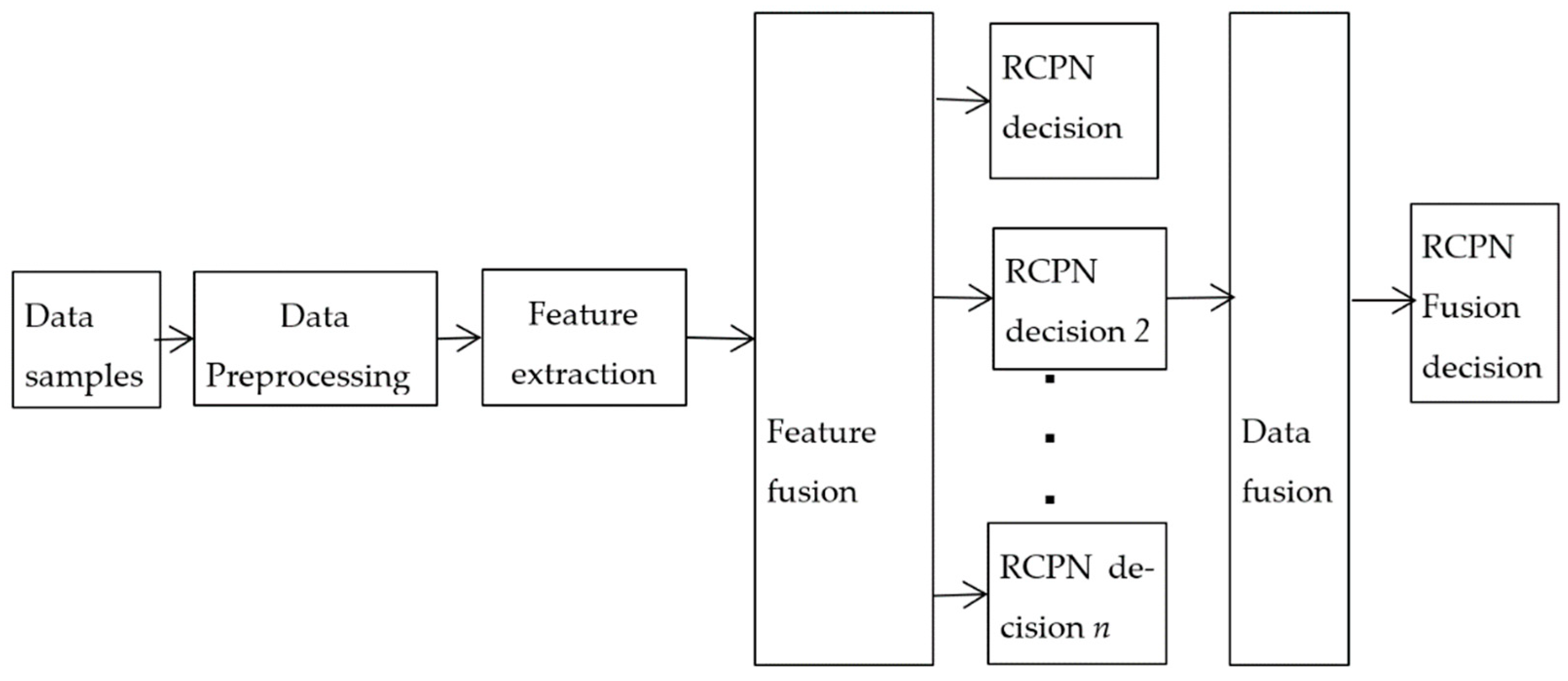
In order to improve the ability of the damage detection method in extracting structural damage features and noise processing—effectively improving the precision of structural damage detection—a structural damage detection method based on fractal dimension, data fusion and RCPN is proposed as shown in Figure 2.

3.1. Data Preprocessing

Considering that in the testing process of the structural health testing system, due to the existence of adverse factors such as testing environment, measurement errors and test technical defects, the test data often contain different degrees of measurement noise and test errors. In order to obtain better damage recognition accuracy, data preprocessing is often necessary. The commonly used methods include the threshold method and average method, which can eliminate mixed noise and errors in test data by preprocessing test signals.

3.2. Fractal Features Extraction

Correlation dimension [37,38,39] is a common dimension used in fractals. Fractal correlation dimension not only represents the degree of density of the system in multidimensional space, but also can reflect the correlation degree between two points of the system. Hence, fractal correlation dimension is often used to describe the characteristic quantity of a system. Since the correlation dimension can reflect the irregularity and complexity of the signal to be analyzed, it can be used to distinguish the classification of structural health state and damage state. Among the methods to obtain the correlation dimension, the G-P algorithm [39,40] is simpler and more reliable than other methods.
The principle of the G-P algorithm to solve the correlation dimension can be expressed by assuming a measured time data series with {x1, x2,…, xN}, where N is the length of the time series signal, the phase–space reconstruction of the original signal data sequence is carried out by using the time-delay method, and its length is Nm. Then, its pseudo-phase-space orbit can be represented by the following formula:
X i = [ x i , x i + τ , x i + 2 τ , , x i + ( m 1 ) τ ] T
where, τ is the time delay; m is embedding dimension; i = 1,2,…, Nm and N m = N ( m 1 ) τ .
Then, the attractor correlation dimension is obtained by the following correlation integral:
C ( r ) = 2 N m ( N m 1 ) N m N m N m N m H ( r X i X j )
where, C(r) is the correlation integral of signal; H is the Heaviside function, when u 0 , H(u) = 1; when u < 0, H(u) = 0; r is the hyperspherical radius of phase space; X i X j is the distance between two vectors:
X i X j = i = 0 m 1 ( x i + l τ x j + l τ ) 1 / 2
Here, the relevant integral C(r) means the probability of a pair of vectors with an embedding space distance less than or equal to r. In addition,
C ( r )   r D 2 r 0
where, D2 is correlation dimension, it can be solved by the following equation:
D 2 = lim ( ln C ( r ) / ln r ) r 0

3.3. Revised Counter-Propagation Network (RCPN)

In view of the above defects of the CPN network model in Section 2, namely, when the two training data values of the input layer are similar, the network connection weight vector may be adjusted twice in each learning, resulting in the failure of the final network training. Reference [36] revised the CPN network model. The improvement process can be summarized as follows: during network training, the samples are trained one by one, that is, a sample is trained first. When the network output error of the sample is less than the set error or reaches the maximum number of iterations, the network training is terminated, and then the next sample is trained until the training of all samples is finished.
After improvement, the defect caused by one connection weight vector being adjusted according to multiple input vectors in the CPN model can be avoided, and each input sample can be successfully trained, and the minimum distance between the connection weight vector of the competing winning neuron and the input mode can be guaranteed. In addition, the number of neurons in the competition layer of the RCPN model is less, and some of them are even equal to the number of samples. Therefore, the structure of the CPN network model is greatly simplified, thus shortening the time of network training and testing [36]. Therefore, in this study, based on the RCPN network model combined with fractal and data fusion, a damage detection model based on decision-level fusion was proposed.

3.4. Fusion Decision and Results Output of RCPN

For a certain test sample A, assume that it contains q pattern categories and the number of sensors is n, and Fj is the total weight of the jth category. Then, the maximum value of total weight in q pattern categories is the output result after fusion:
out = max j = 1 , 2 , q F j
F j = i = 1 n w i , j × f i , j
where, wi,j is the normalized coefficients of sensor i and category j, which is determined by the correct recognition rate of the network model in the training stage and, fi,j is the weight of sensor i and the jth category, and its value is the product of the test sample A in sensor i and the connection weight vector of the jth category, i.e.,
f i , j = m = 1 N a m w i , j , m
where, N is the number of characteristic parameters of test samples, w is the connection weight vector corresponding to sensor i and category j.
According to this method, the RCPN decision results of the feature-level fusion model are taken as the local results of the decision-level fusion model, and the weighted average method is used to fuse the local decision result obtained from all the test samples, and the final decision results after fusion are obtained.

4. Damage Identification of ASCE Benchmark Structure [41]

4.1. Numerical Model

The American Society of Civil Engineers (ASCE) Benchmark structure is a four-storey, 2 × 2 span steel frame structure. Its scaled structure model is shown in Figure 3a. The plane size of the model is 2.5 m × 2.5 m and the height is 3.6m. Each floor and each span of the steel frame model are provided with a floor slab. The four floor slabs of the first floor have a mass of 800 kg, the four floor slabs of the second and third floors have a mass of 600 kg and the four floor slabs of the fourth floor have a mass of 400 kg. In this paper, a structural finite element model of 120 degrees of freedom is adopted, and the schematic diagram of the analysis model is shown in Figure 3b. In the figure, w1, w2 and w3 represent external excitation respectively and are located at the nodes of columns in each layer, y ¨ representing acceleration sensors. Two acceleration sensors are arranged in the x and y directions of each layer, with a total of 16 acceleration sensors. The sampling frequency was 1000 Hz, the sampling duration was 10 s, and the excitation mode was environmental excitation. Four damage modes were simulated, as shown in Table 1.

4.2. Damage Detection Results of Single RCPN Classifier

The Benchmark problem data generation program Datagen was used to simulate various structural damage conditions and generate time-history response data of each damage condition. Based on the measured response data obtained by the Y-direction sensor, the correlation dimension values of each sensor under various damage modes were calculated according to Equation (13) in Section 3.2, which was taken as the damage characteristic parameters and as the input vectors of the RPN network model. Considering the inevitability of noise in actual signal measurement, three noise levels of 30%, 50%, and 70% are generated in the simulation.
y i = y i a ( 1 + ε R )
Here, y i is the acceleration signal after noise pollution; y i a is the measured acceleration signal; R is a normally distributed random number with a mean of 0 and a deviation of 1; ε is the noise degree index, and here, ε is set as 0%, 50% and 70% respectively.
Each damage condition at each noise level generates 1200 samples randomly; that is, each damage mode at each noise level can obtain 1200 correlation dimensions through calculation. These can be divided equally into two groups, namely, the first 6 × 100 data were used as training samples, and the last 6 × 100 data were used as test samples, which were divided into three groups (where each group has two columns, and each column has 100 correlation dimensions), represented by NC1, NC2 and NC3 (where each group has two columns). The RCPN structure of each noise level was the same.
RCPN classifier 1 was taken as an example to illustrate the establishment process of the network model. Firstly, if the input vector is NC1, the number of neurons in the input layer is equal to the number of characteristic parameters of the sample, namely, the number of neurons in the input layer is 2. Secondly, the number of neurons in the output layer is equal to the number of damage modes; there are four damage modes in this paper, so the number of output neurons is four. Finally, the number of neurons in the competition layer is equal to the number of input samples. Since there are 400 samples, the number of neurons in the competition layer is 400, and the structure of the established RCPN model is 2-400-4. The identification accuracy of all training samples is 100%, and the RCPN network training is completed. Here, α and β are both set as 0.1.
There is a test sample A of network input, that is, the input layer provided by ai to the network. The winning neuron g of the neurons in the competition layer can be obtained as follows:
b g = max i = 1 , 2 , , Q ( i = 1 N w j i a i )
Set bg = 1, and the rest of the output equals 0, according to the equation c j = v j g b g , the output of each neuron in the output layer can be obtained. Thus, an output mode C = ( c 1 , c 2 , , c M ) is generated, and the corresponding classification result of the output is the classification result of input A. Damage identification accuracy (IA) is defined here as the ratio of the total number of correctly identified samples to the total number of tested samples. The damage identification results of a single RCPN classifier under various noise levels are shown in Table 2.
It can be seen from Table 2, when the noise levels are 30%, 50% and 70%, respectively, the total average IA of a single RCPN classifier is 91.6%, 87.25% and 78.3%, respectively, with the total average IA all exceeding 78%. This indicates that the correlation dimension as the feature vector for damage identification can receive better recognition effect, and also indicates that the damage feature vector is more sensitive to structural damage. When the noise level is 30%, the comparison of damage identification results of each damage feature vector is shown in Figure 4a. As can be seen from Figure 4a, IA of damage patterns 1 and 2 is relatively high, while that of damage patterns 3 and 4 is slightly lower. The same phenomenon is also observed when the noise level is 50% and 70%, as shown in Figure 4b,c. This is mainly because damage patterns 1 and 2 are both more severe, so are easier to distinguish compared with the other two kinds of damage, so the IA is better.
It can also be seen from Table 2 that when the noise level is 30%, the average IA of feature vectors NC1, NC2 and NC3 is 92.75%, 92% and 90%, respectively. When the noise level is 50%, the average IA of feature vectors NC1, NC2 and NC3 is 87%, 86.75% and 88%, respectively. When the noise level is 70%, the average IA of feature vectors NC1, NC2 and NC3 is 78%, 78.25% and 78.75%, respectively. On the whole, there is little difference in the accuracy of damage identification among the three feature vectors, which also indicates that the RCPN network model has good noise resistance and robustness.

4.3. Damage Detection Results of Feature-Level Fusion Model

Feature-level fusion refers to the feature-level fusion of input vectors of the above single RCPN network model. Then, the fused correlation dimension groups were used as a new feature vector and input into the input layer of the RCPN network model for RCPN calculation, and eventually output the damage recognition results, which were shown in Table 3.
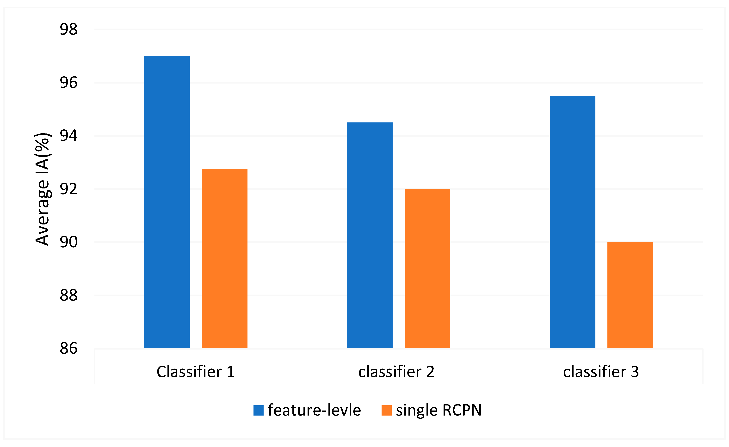
It can be seen from Table 3, after the feature-level fusion, when the noise level is 30%, 50% and 70%, the total average IA of the feature-level fusion damage recognition model is 95.2%, 88.7% and 81.0%, respectively. Moreover, with the increase of noise level, the recognition accuracy of the model decreases correspondingly, which is completely consistent with the reality. Taking a noise level of 30% as an example, the recognition results of a single RCPN classifier and a feature-level fusion model are compared, as shown in Figure 5.
It can also be seen from Table 3 and Figure 5, comparing with single RCPN classifiers, the classifier of feature-level fusion has better improved IA. When the noise level is 30%, the total recognition accuracy of the four feature-level fusion methods is 97%, 94.5%, 95.5% and 93.75%, respectively, with the total average IA exceeding 93%, which is significantly improved compared with the single RCPN network model. Among them, fusion method 1 had the highest damage identification accuracy. This is mainly because, in the identification of a single RCPN model, the total identification accuracy of single feature vectors NC1 and NC2 is high, and these two feature vectors are more sensitive to structural damage. Therefore, after feature-level fusion, the damage identification result is bound to be higher than that of other combination methods. When the noise level is 50%, this phenomenon is also reflected. The damage recognition results of the RCPN model with single feature vectors NC1 and NC3 are better. Therefore, after the feature-level fusion, the damage recognition results after the fusion of two feature vectors are further improved.

4.4. Damage Detection Results of Decision—Level Fusion Model

Structural damage detection using the decision-level fusion model in this paper means that the damage decision results of feature level fusion model were used as the local decision results and eventually the fusion decision results are obtained by decision-level fusion calculation. According to the fusion decision calculation method described in Section 3.4, for a test sample A, the results of data fusion decision is the largest of the total weight among the four damage patterns, namely, o u t = max j = 1 , 2 , 4 F j and, here F j = i = 1 4 w i , j × f i , j ,which is the total weight of the damage pattern j . since the correct recognition rate of RCPN network model in the training process is 100%, then, w i , j was set as 1/3 for all of them. Decision-level data fusion was carried out for each test sample one by one until all damage detection samples were fused. At this time, the output fusion results were the final damage identification results. The damage identification results of RCPN decision-level fusion model were shown in Table 4.
As can be seen from the identification results in Table 4, when the noise level is 30%, the IA of the three decision-level fusion methods are all more than 96%, and the total average IA is 96.9%. The identification results of decision-level RCPN model are satisfactory. When the noise level is 50%, the average IA of the three decision-level fusion methods is 90.25%, 91.75% and 90%, respectively, and the total average IA is 90.7%. When the noise level is 70%, among the three fusion methods, the average IA of the second fusion method is the highest, reaching 85.75%. This is mainly because these two classifiers had obtained better recognition results in feature-level fusion. Therefore, in the calculation of decision-level fusion, the damage recognition results of feature-level fusion were taken as the local decision results to obtain better recognition results. On the whole, even when the noise level is up to 70%, the decision-level fusion damage recognition model still had good anti-noise performance.
It can also be seen from Table 4 that with the increase of noise level, the identification accuracy of decision-level fusion model decreases. Contrary to that, it can be found from the results that, under the same noise level, the decision results obtained by different fusion methods are very close with little difference, which also indicates that the structural damage model based RCPN is insensitive to the feature input vectors and has good robustness.

4.5. Comparison and Discussion

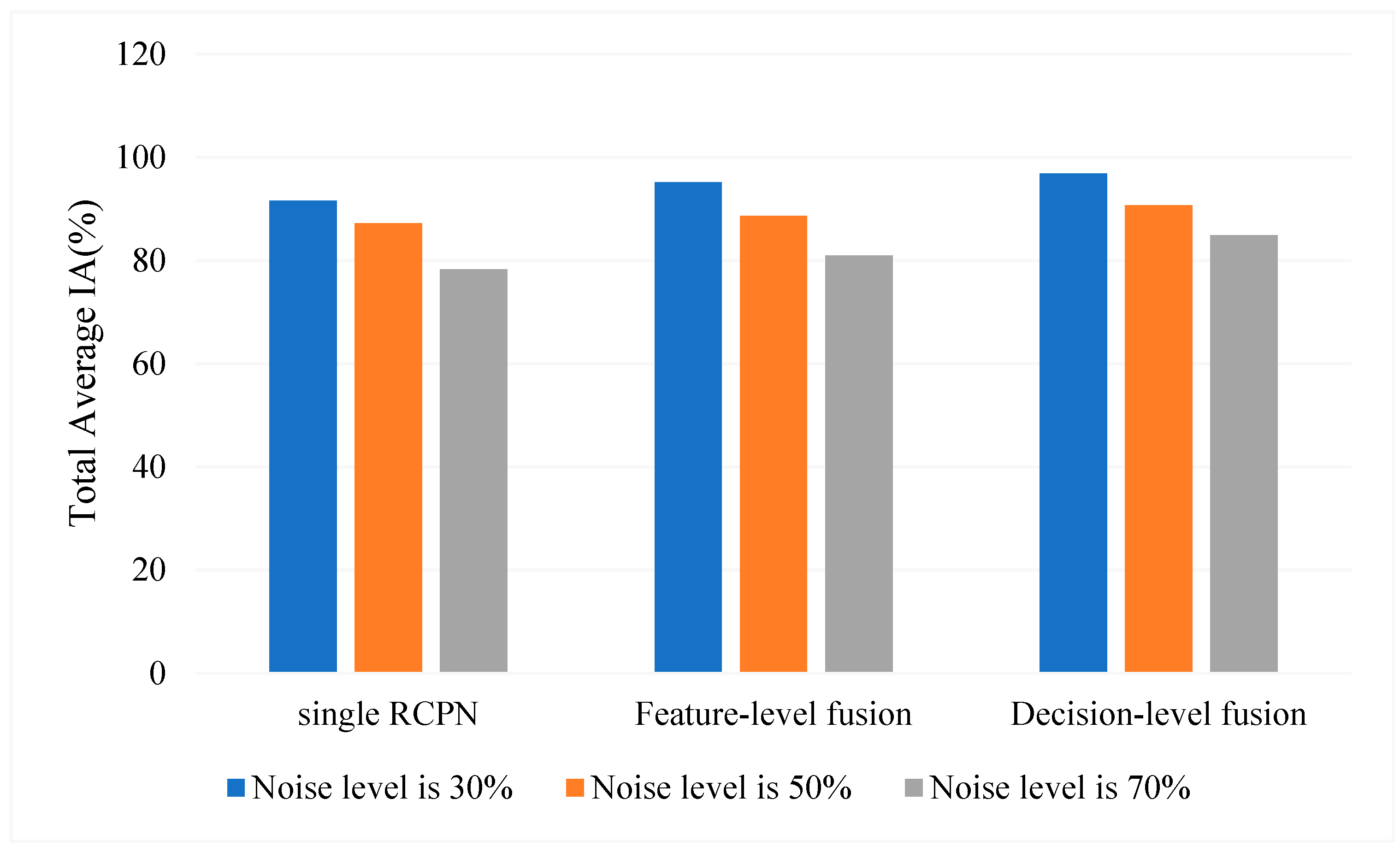
It can be seen from the comparison of structural damage identification results in Table 2, Table 3 and Table 4, with the increase of added noise level, the accuracy of damage identification of the single RCPN classifier model, feature-level fusion model and decision-level fusion model decreases. When the noise levels were 30%, 50% and 70%, the total average IA of the single RCPN classifier was 91.6%, 87.25% and 78.3%, respectively, and the total average IA of the feature level fusion model was 95.2%, 88.7% and 81.0%, respectively. The total average IA of decision-level fusion model is 96.9%, 90.7% and 84.9%, respectively. The comparison of damage identification accuracy is shown in Figure 6.
It can be clearly seen from Figure 6 that for structural damage identification based on correlation dimension, the IA of decision-level fusion model is better than that of feature-level fusion model, and feature-level fusion model is better than the single RCPN model. It can also be seen from Figure 6 that when the noise levels are 30%, 50% and 70%, the total average IA of the feature-level fusion model is 3.6%, 1.45% and 2.7% higher than that of the single RCPN model, respectively. The total average IA of the decision-level fusion model is increased by 1.7%, 2% and 3.9% compared with the feature-level fusion model, and by 5.3%, 3.45% and 6.6% compared with the single RCPN model, respectively. From these comparison results, it can be seen that with the increase of noise level, the total average IA of the feature-level and decision-level fusion model is significantly improved compared with the single RCPN model, indicating that the proposed feature-level fusion model and decision-level fusion model had better noise resistance.
The comparison between Table 3 and Table 4 shows that, when the noise level is 70%, the highest and lowest identification accuracy of the decision-level fusion model is 85.75% and 84%, respectively, while that of the corresponding feature-level fusion model is 81.75% and 80.25%, respectively. Compared with the feature-level fusion model, the average IA of the decision-level fusion model is increased by 5.5% at the highest and 2.25% at the lowest, indicating that the decision-level fusion model has better noise resistance than the feature-level fusion model. Moreover, it can also be seen from Table 3 and Table 4, for different damage indexes, the IA at the same noise level has little difference, which indicates that the two structural damage models are insensitive to damage feature vectors and have good robustness.

5. Conclusions

In this paper, a decision-level fusion method for structural damage identification is proposed based on correlation dimension and RCPN. The Benchmark structure of the ASCE is used to verify the potential of correlation dimension as a structural damage identification feature.
The research results showed that after data fusion, both the feature-level fusion damage identification model and the decision-level fusion damage identification model are significantly superior to the identification results of a single RCPN model. Particularly, the decision-level fusion damage detection model proposed in this paper based on the feature-level fusion results can significantly improve the accuracy of structural damage identification. It has the best identification accuracy, noise resistance and robustness among the three models. However, it is worth noting that the proposed model in this paper is only proved to be feasible and effective in numerical examples, its actual performance in experimental work needs to be further studied.
In the following research work, low-degree damage will be identified, and it is planned to be combined with decision tree, random forest, deep neural network and other methods to improve the accuracy of damage identification. In future, we will continue to carry out multiple damage identification and prediction and devote ourselves to applying our research results in practical experiments and engineering.

Author Contributions

Conceptualization, C.F. and M.L.; methodology, C.F.; software, C.F.; validation, C.F.; writing—original draft preparation, C.F.; writing—review and editing, C.F.; visualization, C.F. and M.L.; supervision, M.L.; project administration, C.F. and M.L.; funding acquisition, C.F. and M.L. All authors have read and agreed to the published version of the manuscript.

Funding

This research was funded by Basic Scientific Research Project of Education Department of Liaoning Province (LJKMZ20220750). Liaoning Provincial Department of Education Project (LJKZ056); and Housing and Rural Construction Project (2019-K-080).

Data Availability Statement

The data presented in this study are available upon request from the corresponding author.

Acknowledgments

Thanks to the Shaofei Jiang from Fuzhou University for his help in this research.

Conflicts of Interest

The authors declare no conflict of interest.

References

  1. Wang, H.; Tao, T.; Li, A.; Zhang, Y. Structural health monitoring system for Sutong Cable-stayed Bridge. Smart Struct. Syst. 2016, 18, 317–334. [Google Scholar] [CrossRef]
  2. Liu, T.; Xu, H.; Ragulskis, M.; Cao, M.; Ostachowicz, W. A Data-Driven Damage Identification Framework Based on Transmissibility Function Datasets and One-Dimensional Convolutional Neural Networks: Verification on a Structural Health Monitoring Benchmark Structure. Sensors 2020, 20, 1059. [Google Scholar] [CrossRef] [PubMed]
  3. Zhang, Y.M.; Wang, H.; Wan, H.P.; Mao, J.X.; Xu, Y.C. Anomaly detection of structural health monitoring data using the maximum likelihood estimation-based Bayesian dynamic linear model. Struct. Health Monit. 2021, 20, 2936–2952. [Google Scholar] [CrossRef]
  4. Scianna, A.M.; Christenson, R. Probabilistic Structural Health Monitoring Method Applied to the Bridge Health Monitoring Benchmark Problem. Transport. Res. Rec. 2018, 2131, 92–97. [Google Scholar] [CrossRef]
  5. Alrasheedi, A.F.; Alnowibet, K.A.; Saxena, A.; Sallam, K.M.; Mohamed, A.W. Chaos Embed Marine Predator (CMPA) Algorithm for Feature Selection. Mathematics 2022, 10, 1411. [Google Scholar] [CrossRef]
  6. Dessi, D.; Camerlengo, G. Damage identification techniques via modal curvature analysis: Overview and comparison. Mech. Syst. Signal Process. 2015, 52–53, 181–205. [Google Scholar] [CrossRef]
  7. Feng, D.; Feng, M.Q. Output-only damage detection using vehicle-induced displacement response and mode shape curvature index. Struct. Control Health Monit. 2016, 23, 1088–1107. [Google Scholar] [CrossRef]
  8. Stutz, L.; Rangel, I.; Rangel, L.; Corrêa, R.; Knupp, D. Structural damage identification built on a response surface model and the flexibility matrix. J. Sound Vib. 2018, 434, 284–297. [Google Scholar] [CrossRef]
  9. Ghannadi, P.; Kourehli, S.S. Structural damage detection based on MAC flexibility and frequency using moth-flame algorithm. Struct. Eng. Mech. 2019, 70, 649–659. [Google Scholar]
  10. Li, Y.; Cheng, L.; Yam, L.; Wong, W.O. Identification of damage locations for plate-like structures using damage sensitive indices: Strain modal approach. Comput. Struct. 2002, 80, 1881–1894. [Google Scholar] [CrossRef]
  11. Thue Nguyen, Q.; Livaŏglu, R. Modal strain energy based enhanced approaches for damage detection and severity estimation. Eng. Fail. Anal. 2023, 146, 107142. [Google Scholar] [CrossRef]
  12. Gillich, G.-R.; Praisach, Z.-I. Modal identification and damage detection in beam-like structures using the power spectrum and time–frequency analysis. Signal Process. 2014, 96, 29–44. [Google Scholar] [CrossRef]
  13. Yu, Z.; Xia, H.; Goicolea, J.M.; Xia, C. Bridge Damage Identification from Moving Load Induced Deflection Based on Wavelet Transform and Lipschitz Exponent. Int. J. Struct. Stab. Dyn. 2016, 16, 1550003. [Google Scholar] [CrossRef]
  14. Sun, G.; Wang, Y.; Luo, Q.; Li, Q. Vibration-based damage identification in composite plates using 3D-DIC and wavelet analysis. Mech. Syst. Signal Process. 2022, 173, 108890. [Google Scholar] [CrossRef]
  15. Lo Iacono, F.; Navarra, G.; Pirrotta, A. A damage identification procedure based on Hilbert transform: Experimental validation. Struct. Control Health Monit. 2012, 19, 146–160. [Google Scholar] [CrossRef]
  16. Xiang, H.; Nie, Z.; Gao, R.; Ma, H. Pattern Matching-Based Structural Damage Identification Using Mode Shape Difference Ratio with Limited Sensors. Int. J. Struct. Stab. Dyn. 2023, 1–23, 2350106. [Google Scholar] [CrossRef]
  17. Zhang, Z.; Sun, C.; Guo, B. Transfer-learning guided Bayesian model updating for damage identification considering modeling uncertainty. Mech. Syst. Signal Process. 2021, 166, 108426. [Google Scholar] [CrossRef]
  18. Shi, B.; Qiao, P. A new surface fractal dimension for displacement mode shape-based damage identification of plate-type structures. Mech. Syst. Signal Process. 2018, 103, 139–161. [Google Scholar] [CrossRef]
  19. Huang, Y.; Li, H.; Wu, S.; Yang, Y. Fractal dimension based damage identification incorporating multi-task sparse Bayesian learning. Smart Mater. Struct. 2018, 27, 075020. [Google Scholar] [CrossRef]
  20. Ramezani, M.; Bahar, O. Structural damage identification for elements and connections using an improved genetic algorithm. Smart Struct. Syst. 2021, 28, 643–660. [Google Scholar]
  21. Ghannadi, P.; Kourehli, S.S.; Mirjalili, S. The Application of PSO in Structural Damage Detection: An Analysis of the Previously Released Publications (2005–2020). Frat. Ed Integrità Strutt. 2022, 16, 460–489. [Google Scholar] [CrossRef]
  22. Lei, Y.; Zuo, M.J. Gear crack level identification based on weighted K nearest neighbor classification algorithm. Mech. Syst. Signal Process. 2009, 23, 1535–1547. [Google Scholar] [CrossRef]
  23. Sarmadi, H.; Karamodin, A. A novel anomaly detection method based on adaptive Mahalanobis-squared distance and one-class kNN rule for structural health monitoring under environmental effects. Mech. Syst. Signal Process. 2019, 140, 106495. [Google Scholar] [CrossRef]
  24. Lei, J.; Cui, Y.; Shi, W. Structural damage identification method based on vibration statistical indicators and support vector machine. Adv. Struct. Eng. 2022, 25, 1310–1322. [Google Scholar] [CrossRef]
  25. Ren, J.; Zhang, B.; Zhu, X.; Li, S. Damaged cable identification in cable-stayed bridge from bridge deck strain measurements using support vector machine. Adv. Struct. Eng. 2022, 25, 754–771. [Google Scholar] [CrossRef]
  26. Rabiej, M.; Rabiej, S. Application of the artificial neural network for identification of polymers based on their X-ray diffraction curves. Comput. Mater. Sci. 2020, 186, 110042. [Google Scholar] [CrossRef]
  27. Ye, L.; Su, Z.; Yang, C.; He, Z.; Wang, X. Hierarchical development of training database for artificial neural network-based damage identification. Compos. Struct. 2006, 76, 224–233. [Google Scholar] [CrossRef]
  28. González-Pérez, C.A.; González, J.V. Identification of Structural Damage in a Vehicular Bridge using Artificial Neural Networks. Struct. Health Monit. 2010, 10, 33–48. [Google Scholar] [CrossRef]
  29. Li, J.; Dackermann, U.; Xu, Y.-L.; Samali, B. Damage identification in civil engineering structures utilizing PCA-compressed residual frequency response functions and neural network ensembles. Struct. Control Health Monit. 2015, 18, 207–226. [Google Scholar] [CrossRef]
  30. Gu, J.; Gul, M.; Wu, X. Damage detection under varying temperature using artificial neural networks. Struct. Control. Health Monit. 2017, 24, e1998. [Google Scholar] [CrossRef]
  31. Aziz, R.M.; Mahto, R.; Goel, K.; Das, A.; Kumar, P.; Saxena, A. Modified Genetic Algorithm with Deep Learning for Fraud Transactions of Ethereum Smart Contract. Appl. Sci. 2023, 13, 697. [Google Scholar] [CrossRef]
  32. Sony, S.; Gamage, S.; Sadhu, A.; Samarabandu, J. Multiclass Damage Identification in a Full-Scale Bridge Using Optimally Tuned One-Dimensional Convolutional Neural Network. J. Comput. Civ. Eng. 2022, 36, 04021035. [Google Scholar] [CrossRef]
  33. Li, D.; Liang, Z.-L.; Ren, W.-X.; Yang, D.; Wang, S.-D.; Xiang, S.-L. Structural damage identification under nonstationary excitations through recurrence plot and multi-label convolutional neural network. Measurement 2021, 186, 110101. [Google Scholar] [CrossRef]
  34. Puruncajas, B.; Vidal, Y.; Tutivén, C. Vibration-Response-Only Structural Health Monitoring for Offshore Wind Turbine Jacket Foundations via Convolutional Neural Networks. Sensors 2020, 20, 3429. [Google Scholar] [CrossRef] [PubMed]
  35. Agrawal, S.; Singh, R.K.; Singh, U.P.; Jain, S. Biogeography particle swarm optimization based counter propagation network for sketch based face recognition. Multimedia Tools Appl. 2018, 78, 9801–9825. [Google Scholar] [CrossRef]
  36. Jiang, S.F.; Lin, J. Structural damage identification based on rough set and revised counter-propagation network. J. Vib. Shock 2011, 30, 1–645. [Google Scholar]
  37. Zhou, L.; Sun, H.; He, Z. Fractal dimension-based damage imaging for composites. Shock Vib. 2013, 20, 164539. [Google Scholar] [CrossRef]
  38. Wang, Y.; Yan, C.; Zhang, T.; Wang, N.; Chen, L.; Jie, G. Acoustic emission fractal characteristics analysis of steel fiber reinforced concrete during uniaxial tensile damage. Mater. Test. 2020, 62, 329–336. [Google Scholar] [CrossRef]
  39. Woods, J.E.; Yang, Y.-S.; Chen, P.-C.; Lau, D.T.; Erochko, J. Automated Crack Detection and Damage Index Calculation for RC Structures Using Image Analysis and Fractal Dimension. J. Struct. Eng. 2021, 147, 04021019. [Google Scholar] [CrossRef]
  40. Rolo, A. A method for the correlation dimension estimation for on-line condition monitoring of large rotating machinery. Mech. Syst. Signal Process. 2005, 19, 939–954. [Google Scholar] [CrossRef]
  41. Johnson, E.A.; Lam, H.F.; Katafygiotis, L.S.; Beck, J.L. Phase I IASC-ASCE Structural Health Monitoring Benchmark Problem Using Simulated Data. J. Eng. Mech. 2004, 130, 3–15. [Google Scholar] [CrossRef]
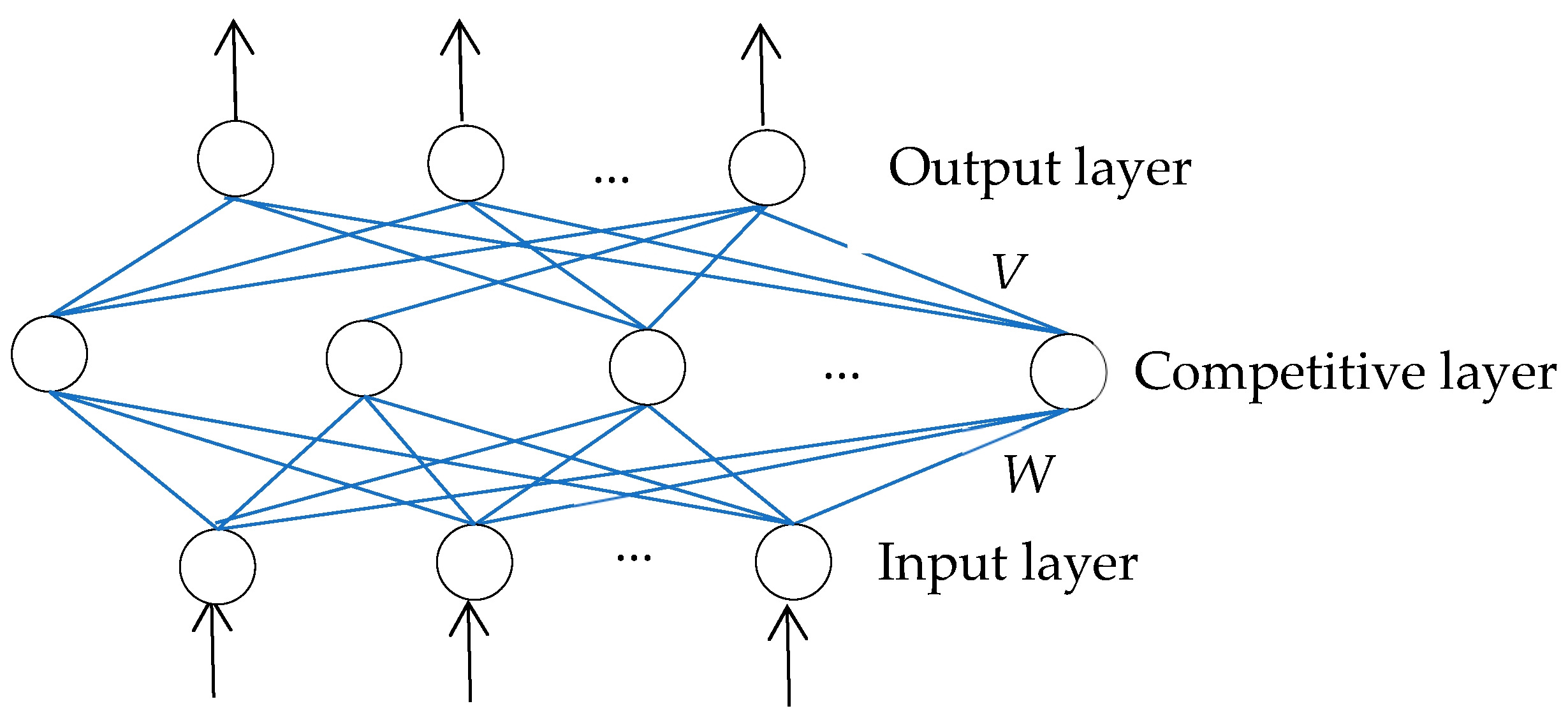
Figure 1. CPN model structure.
Applsci 13 05289 g001
Figure 2. Structural damage detection method.
Applsci 13 05289 g002
Figure 3. ASCE benchmark structural model [41]. (a) Experimental model of steel frame. (b) Analysis model.
Applsci 13 05289 g003
Figure 4. Comparison of the accuracy of damage pattern recognition when the noise level is 30%, 50% and 70% respectively. (a) Noise level ε = 30%. (b) Noise level ε = 50%. (c) Noise level ε = 70%.
Applsci 13 05289 g004aApplsci 13 05289 g004b
Figure 5. Comparison of the accuracy of damage between feature-level and single RCPN when the noise level is 30%.
Applsci 13 05289 g005
Figure 6. Comparison of damage identification accuracy of three models.
Applsci 13 05289 g006
Table 1. Structural damage simulation scenarios.
Damage PatternDamage Simulation
1Remove all support from the first layer
2Remove all supports from Layers 1 and 3
3Remove 1 brace from 1st layer
4Remove 1 brace each from the 1st and 3rd layers
Table 2. Damage identification results of a single RCPN classifier.
Noise Level ε (%)ClassifierIA of Damage Patterns (%)Average IA(%)Total Average IA
(%)
Pattern 1Pattern 2Pattern 3Pattern 4
30NC19694919092.7591.6
NC29195899392
NC39491838890
50NC1938985818787.25
NC29095808286.75
NC38991848888
70NC1838571737878.3
NC28187747178.25
NC38285737578.75
Table 3. Feature level fusion damage identification results of RCPN.
Noise Level ε (%)Feature-Level Fusion MethodsIA of Damage Patterns (%)Average IA(%)Total Average IA
(%)
Pattern 1Pattern 2Pattern 3Pattern 4
30Classifier 1 (NC1 + NC2)999997969795.2
Classifier 2 (NC2 + NC3)9797919394.5
Classifier 3 (NC1+NC3)9896949495.5
Classifier 4 (NC1 + NC2 + NC3)9698919093.75
50Classifier 1 (NC1 + NC2)9497828188.588.7
Classifier 2 (NC2 + NC3)9692808287.5
Classifier 3 (NC1 + NC3)9595858790.5
Classifier 4 (NC1 + NC2 + NC3)9394818588.25
70Classifier 1 (NC1 + NC2)8785767580.7581.0
Classifier 2 (NC2 + NC3)8789757481.25
Classifier 3 (NC1 + NC3)8488767981.75
Classifier 4 (NC1 + NC2 + NC3)8386787480.25
Table 4. Decision-level damage identification results of RCPN.
Noise Level ε (%)Decision-Level Fusion MethodsIA of Damage Patterns (%)Average IA(%)Total Average IA
(%)
Pattern1Pattern2Pattern 3Pattern4
301 (classifier 1 + 2)9899979697.596.9
2 (classifier 2 + 3)9998969597
3 (classifier 1 + 2 + 3)9897959596.25
501 (classifier 1 + 2)9696848590.2590.7
2 (classifier 2 + 3)9795868991.75
3 (classifier 1 + 2 + 3)9695848590
701 (classifier 1 + 2)909278808584.9
2 (classifier 2 + 3)9191798285.75
3 (classifier 1 + 2 + 3)8990787984
Disclaimer/Publisher’s Note: The statements, opinions and data contained in all publications are solely those of the individual author(s) and contributor(s) and not of MDPI and/or the editor(s). MDPI and/or the editor(s) disclaim responsibility for any injury to people or property resulting from any ideas, methods, instructions or products referred to in the content.