Abstract
The thermal error modeling technology of computer numerical control (CNC) machine tools is the core of thermal error compensation, and the machining accuracy of CNC machine tools can be improved effectively by the high-precision prediction model of thermal errors. This paper analyzes several methods related to thermal error modeling in the latest research applications, summarizes their deficiencies, and proposes a thermal error modeling method of CNC machine tool based on the improved particle swarm optimization (PSO) algorithm and radial basis function (RBF) neural network, named as IPSO-RBFNN. By introducing a compression factor to make the PSO algorithm balance between global and local search, the structure parameters of RBF neural network are optimized. Furthermore, in order to pick up the temperature-sensitive variables, an improved model, which combines the K-means clustering algorithm and correlation analysis method based on back propagation (BP) neural network is proposed. After the temperature-sensitive variables are selected, the IPSO-RBFNN method is adopted to establish the thermal error model for CNC machine tool. Based on the experimental data of the CNC machine tool under the name of DMG-DMU65, the predictive accuracy of the IPSO-RBFNN model in Z direction reaches 2.05 μm. Compared with other neural network method, it is improved by 10.48%, which indicates that it has better prediction ability. At last, the experiment verification for different thermal error terms at different velocities proves that this model has stronger robustness.
1. Introduction
Precise Computer Numerical Control (CNC) machine tool has symbolic significance for the standard of modern machining, and its importance is on the rise. With the sustaining progress of industrial technology, the demands for the accuracy of CNC machine tool are increased synchronically. Many factors have vital effects on the accuracy of machine tools, including geometric errors, thermal errors, cutting-force induced errors and others [1].
According to Ramesh’s research [2] published in 2000, it was discovered that thermal errors affected the machining accuracy remarkably, accounting for 45–65% of total errors. Apparently, it is crucial to study the methods to eliminate the effect of thermal errors [3].
Thermal error occurs when the thermal expansion of machine tool components causes displacement of the cutter relative to the workpiece [4]. In order to decrease thermal error, scholars carry out research from two aspects at present: error prevention and error compensation [5]. The former is to decrease or even eliminate the possibility of thermal error by promoting design and manufacturing level, such as adopting advanced materials [6], separating heat source [7] and so on. Considering that the use of these methods will lead to an exponential increase in manufacturing costs, it is difficult to utilize them practically. The error compensation method mainly studies the relationship between thermal errors and temperatures of critical heat source through analysis and statistics, thereby establishing the predictive model of thermal errors and using for compensation [8]. In comparison with the way of error prevention, it is more economical and appropriate to decrease the thermal errors through compensation [9].
The aim of thermal error compensation is to establish thermal error model with high predictive performance for different working conditions. The modeling method for thermal errors of the CNC machine tool mainly includes two aspects: empirical modeling and theoretical modeling [10]. The theoretical modeling method requires analysis of the thermal mechanism, the distribution of temperature field of overall machine tool and the main parts, and calculation of the boundary conditions. Because of the complex deformation process, it is difficult to establish a strict model to simulate the thermal deformation of machine tool. In addition, when the terminal conditions are hard to determine, the predictive performance of the theoretical model may be poor. Therefore, empirical modeling method is more frequently used to establish the thermal errors of machine tool. To build a thermal error prediction model for machine tool through empirical modeling method, sensors are installed in multiple locations on machine tools to detect the temperature variations, taken as input variables of the model. Contrastively, thermal errors are considered as output variables. By analyzing the correlation between temperature measurements and thermal errors based on statistical models, thermal errors can be predicted by temperature measurements. In this way, thermal error compensation is realized and the precision of CNC machine tool is remarkably promoted.
According to this exploratory direction, tremendous endeavors have been devoted to build predictive models statistically over the last two decades, such as least squares (LS), multivariable regression analysis (MRA), gray system theory (GS), support vector machine (SVM), neural network, and so on.
LS is one of the most widely used methods for thermal error compensation of machine tool, which is applied to find the best function matching to data by finding the sum of the squares of errors minimal [11]. The LS mothed is theoretically mature and structurally simple. However, the predictability of this method under complex conditions is limited because of fewer independent variables.
In comparison with the LS method, there are more independent variables in the MRA model [12]. It is more effective and practical to use the optimal combination of several independent variables to predict the dependent variables. Hence, the model of thermal error established through MRA method brings about higher precision and stronger robustness. However, when involving massive variables, the computation of MRA method is time-consuming and the correlation between thermal errors and temperature variables is merely taken into account, which will result in the coupling of temperature variables and reduce the precision of the model.
The modeling method based on GS theory is simpler and independent of the massive data information [13]. The problem of using GS theory for thermal error modeling is that the model predicts self-development on the basis of its own raw data. As a result, picking altered data from the primary data series will make a big difference to the model.
The SVM method that possesses excellent capability in nonlinear fitting [14] is deemed to be an appropriate model for predictive learning in small samples. However, it is hard to optimize the selection of parameters when utilizing SVM method for thermal error modeling. Moreover, the solving process is resource-consuming and slow.
Generally speaking, neural network has advantages over LS and MRA in the predictive accuracy. There are two common neural network methods: back propagation (BP) and radial basis function (RBF). BP neural network can be used to completely approximate complex nonlinear relations, which contributes to its wide application in thermal error modeling [15]. However, BP neural network has a slow convergence rate and is liable to descend into the local extremum. Furthermore, the initial value is also hard to determine.
As a feedforward neural network, RBF neural network has simple structure and good performance in approximation and global optimization [16]. However, compared with BP neural network, its key feature function is hard to be extracted and its generalization capability is poor.
In order to optimize the initial structural arguments of RBF neural network, particle swarm optimization (PSO) algorithm is adopted because it can iteratively update and change the moving direction of particles to seek optimal solution. PSO algorithm, that is one of the most commonly used metaheuristics in process optimization, has high computational efficiency and requires less adjustment of parameters. As a result, it is considered as a random optimization algorithm with high robustness, and is widely used in function optimization [17,18], neural network training [19,20], fuzzy system control [21,22], and other applications of genetic algorithms [23,24,25]. However, due to the lack of sophisticated search methods, PSO algorithm often cannot get accurate results or guarantee convergence to the global optimum.
In order to overcome the premature convergence of PSO algorithm and other related algorithms mentioned above, an improved PSO-RBF neural network (IPSO-RBFNN) model is proposed for thermal error prediction of machine tools in this paper. In this model, compression factors are used to effectively control the particle velocity and balance the solutions between local and global search. Based on the improved PSO algorithm, the initial structural arguments of RBF neural network are optimized. It turns out that the IPSO-RBFNN model for thermal error prediction has better predictive performance.
The following is the organizational structure of the rest of the article. Literature review for this study is presented in Section 2. The thermal error experiment on a 5-axis CNC machine tool, named as DMG-DMU65, is described in Section 3. The technical specifics of the IPSO-RBFNN model are provided in Section 4. The comparisons of the IPSO-RBFNN model with other models on the basis of the experimental data are conducted in Section 5. In Section 6 the experimental verification under different experimental conditions is carried out to demonstrate the predictive performance and robustness of the model. At last, Section 7 highlights the conclusions and provides an outlook on future research.
2. Literature Review
Over the last two decades, many mathematical modeling methods have been utilized to establish thermal error models of machine tools, such as least square method, multiple regression, grey system, support vector machine, neural network and so on.
In 2015, Li et al. [26] used the Chebyshev polynomial-based orthogonal least squares regression to fit the thermal drift error curve of the spindle. The obtained curve fit well with the measurement error curve. In 2018, Josef May et al. [27] used the weighted least square adaptive parameter updating method to adapt the model parameters and boundary condition changes, to process a random set of sample rates from any measurement of tool center point deviations. Thus, the optimum order of the model was determined and the thermal errors of the five-axis machine tool were predicted. During the 88 h experimental survey, the compensation reduced the occurrence of errors by more than 95%. In addition, with the use of the least square method in 2020, Liu et al. [28] established the radial and axial thermal error model for the spindle of machine tool and carried out error compensation. As a result, the accuracy of workpiece contour was increased by 78.4% after compensation.
In 2011, the multiple regression model was used by Pajor et al. [29] to construct an analytic model of the machine tool spindle. After it was applied for compensation, the thermal error of the spindle declined from 73 μm to 13 μm. In 2020, Liu et al. [30] put forward a thermal error model of linear axis on the basis of regression analysis, which separated thermal error from geometric error. Based on the homogeneous coordinate transformation data, the thermal error compensation method of machine tool was proposed. In comparison with uncompensated conditions, the machining error of the machine tool declined by 85%. Furthermore, in the paper by Shi et al. [31] published in 2022, the traditional multiple linear regression model was improved, and a modeling and compensation method based on the size error of machined parts was proposed. Accordingly, a generalized model of thermal error compensation for machine tool in X direction was established, which realized real-time thermal error compensation, and contributed to a decrease of nearly 52% in the machining error of machined parts.
On the basis of the standard gray system model GM(1, 1), Jiang and his colleagues [32] used a genetic algorithm to optimize the dimensions and weights of the variables in 2010, so as to minimize the residuals of the optimized model. It was able to reflect the tendency of thermal errors systematically, as well as lessen the effect of the stochastic change in thermal error, which contributed to a large promotion of the predictive accuracy of the thermal error model. In order to make the solution of grey prediction model GM(1, N) more accurate, Tien et al. [33] adopted gray control variables, which are more accurate due to their linear gray differential equation, and the corresponding solution based on the superposition principle. To have a higher predictive accuracy, a new gray GMC(1, N) model based on the cuckoo search algorithm, named as CS-GMC(1, N), was proposed for thermal error of machine tool by Wang et al. [34] in 2020. Comparing with the gray model based on PSO, it had a higher predictive accuracy.
Based on SVM, Miao et al. [35] proposed the thermal error model for the spindle of a machining center in 2013, and used it for thermal error compensation, which indicated that the SVM model had good performance on accuracy and robustness. In order to improve the performance of the thermal error model based on SVM, the grid search method was coupled with the SVM model to optimize its penalty and kernel parameters in the article by Zhang et al. [36] published in 2017. By applying the improved SVM model to the CNC machine tool, the positioning errors of X axis and Z axis were decreased by 89.55% and 85.67% respectively. In 2022, Li et al. [37] established the least squares SVM (LS-SVM) prediction model optimized by Aquila Optimizer (AO), which surmounted the problem of prediction error generated by the subjective key parameters of the LS-SVM model, and brought about an average increase of 7.25% in the predictive accuracy of the machine tool motorized spindle thermal errors.
For the purpose of optimizing the thresholds and weights of the BP neural network, the PSO algorithm with variable inertia factor was adopted by Huang et al. [38] to establish the thermal error model for the machine tool in 2014. As a result, the improved BP neural network model was capable of overcoming the restrictions of conventional BP neural network model, which gave rise to a higher predictive accuracy of 93.15%. Considering that BP neural network could not adjust separate arguments according to data updates in thermal error modeling, a revised BP neural network was proposed on the basis of global adjustment tactics by Liu et al. [39] in 2020. By minimizing the square error of whole data, the revised BP neural network model induced a 50% increase in predictive accuracy. Furthermore, in the study by Su et al. [40] in 2011, the RBF neural network was adopted to make the established thermal error model more accurate. However, large amount of time was spent in determining the quantity of neurons in the hidden layer. For promoting the predictive precision of the RBF neural network model, Zhang et al. [41] put forward an improved RBF neural network model for the thermal error prediction in 2019, in which the PSO method was adopted to optimize the key arguments of the RBF neural network.
Moreover, other improvements to the neural network have been made, such as deep learning convolutional neural network (CNN). Deep learning architectures are multilayer stacks of simple modules that allow computational models to learn data expression with multilevel abstraction [42]. Deep learning CNN has generated many breakthroughs in image processing [43,44], finance [45,46] and data mining [47,48]. Based on deep learning CNN, Wu et al. [49] proposed the axial and radial thermal error models for machine tool spindle, coupled with thermal images and thermocouple data to reflect the temperature field of the spindle. The results indicated that the predictive precision of the thermal error model may reach 90~93%.
3. Thermal Error Experiment
In this experiment, 20 batches were measured under different spindle velocities and ambient temperatures. The experimental subject is introduced in Section 3.1 and the experimental data are analyzed in Section 3.2.
3.1. Experiment Subject
The thermal error experiment was carried out on a five-axis CNC machine tool named as DMG-DMU65, and the thermal error of its spindle was detected using the five-point measurement method according to ISO 230-3:2020 [50]. In this way, the thermal error data in the X, Y and Z directions were obtained. In practice, the temperature change area includes not only the spindle area, but also other heat source areas, so it is essential to settle a certain amount of temperature transducers in the non-spindle area. Consequently, 15 temperature transducers were arranged on the CNC machine tool in the spindle area, spindle box area, machine box area, and working table, as shown in Figure 1.
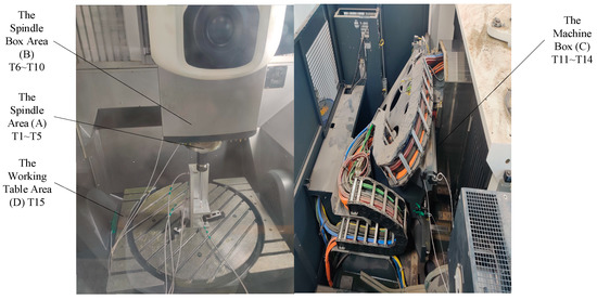
Figure 1.
Temperature transducers arrangement area.
The placement of the temperature transducers placed on the CNC machine tool is shown in Figure 2, and their location distribution is listed in Table 1. It should be noted that, T16 is arranged on the surface of machine tool to detect the ambient temperature, so it is not displayed in Figure 1. T1–T16 are platinum resistors transducers under the name of PT100 with a calibrated precision of 0.01 °C.

Figure 2.
Placement of temperature transducers placed on the CNC machine tool.

Table 1.
Detailed installment location of transducers.
Five eddy current displacement sensors under the name of ML33-02-00-03 were used as the X1, X2, Y1, Y2 and Z displacement measuring components of the spindle of the machine tool respectively. They were installed with customized fixture, as shown in Figure 3. The precision of the sensors can reach 0.1 μm after calibration. In addition, the standard test bar replaced the cutter as the test object, and thermal errors of the spindle that were transferred to the check bar were manifested as its axial and radial displacement.
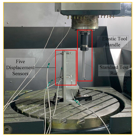
Figure 3.
Displacement sensors arrangement on the CNC machine tool.
3.2. Data Analysis
In total, 20 batches of experiments were carried out, marked as B1–B20. Each batch of experiments was run at five different spindle velocities and four different ambient temperatures. Furthermore, the measurement of each batch includes temperatures and thermal errors. The 20 batches are displayed in an ascending order of velocity, as shown in Table 2.
Table 2.
Experiment conditions of 20 batches.
Figure 4 demonstrates the error curves in X1, X2, Y1, Y2 and Z direction of B5. It is observed that thermal errors of X1, X2, Y1 and Y2 direction rise rapidly to around the 60th minute. After that, the curves flatten out, while the thermal error of Z direction peaks around 140 min and then declines slowly. Since thermal errors due to axial thermal expansion of the spindle of machine tool account for a majority of the entire thermal errors [51], the thermal error in Z direction is taken as the priority of the research in this paper. In the following section, the methodology is presented to pick up temperature-sensitive variables and establish the model between thermal errors and temperature transducers.
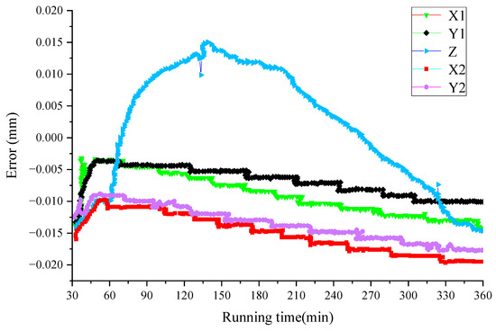
Figure 4.
Thermal error curves in X1, X2, Y1, Y2 and Z direction of B5.
4. Methodology
As mentioned above, the RBF neural network that has strong nonlinear mapping capability can effectively reflect the nonlinear relation between temperature variables and thermal errors of the spindle. For optimizing the structure parameters of the RBF neural network so that the predictive accuracy of the thermal error model for the spindle is promoted, the IPSO-RBFNN model is proposed in thermal error modeling by combining the improved PSO algorithm with the RBF neural network. Prior to establishing the thermal error model, an improved method, described in Section 4.1, is used to pick up the temperature-sensitive variables from the 16 installed transducers. The IPSO-RBFNN model, utilizing the selected temperature-sensitive variables, is used for thermal error modeling, and is presented in Section 4.2.
4.1. Temperature-Sensitive Variable Selection
To screen the temperature-sensitive points, considering different heat sources, an improved method that is proposed in this section combines the K-means clustering algorithm [52] and correlation analysis method [53] based on BP neural network, named as KR-BPNN.
4.1.1. K-Means Clustering Algorithm
Suppose, the sample X = {x1, x2,…, xn} of N objects, and the dimension of each object is M. K-means clustering aims to classify N objects into K clusters based on the similarity of samples and ensure that one object belongs to only one cluster. The steps of K-mean clustering are as follows:
Step 1: Initializing the clustering center, and selecting K objects randomly as the clustering center {C1, C2, …, Cn}, where 1 < k ≤ n.
Step 2: Calculating the distance between K objects and the centers of each cluster based on Euclidean distance.
where, xi is the ith object (1 ≤ i ≤ n); Cj is the Jth clustering center (1 ≤ j ≤ k); xil is the attribute of the lth (1 ≤ l ≤ m) dimension of the ith object; and Cjl is the attribute of the lth dimension of the Jth cluster center.
Step 3: According to the Euclidean distance of each object to the center of each cluster, it is classified into clusters with minimal distance, based on which K clusters {S1, S2, …, Sk} are obtained.
Step 4: Calculating the mean of all objects in the clusters and using this value as the center of the new cluster.
where, Cp is the pth (1 ≤ p ≤ k) new cluster center; |Sp| is the object number of the lth cluster; and xi is the ith object in the pth cluster.
Step 5: Judging whether the gap between the new and old cluster centers is small or iteration is completed. If yes, the algorithm ends. Otherwise, repeat steps 2~5.
4.1.2. Correlation Analysis Method
Correlation analysis mainly studies the correlation between multiple variables. It is often expressed by correlation coefficient R. For the continuity between temperature variables and thermal errors, the Pearson correlation coefficient [54] is adopted to represent the correlation between them. Equation (3) is the formula of the Pearson correlation coefficient.
where, Rxy is the correlation coefficient of the object; Sxy is the covariance of the object; Sx is the standard deviation of sample X of the temperature variables; Sy is the standard deviation of sample Y of thermal errors; N is the sample size; Xi is the ith temperature variable; is the mean of all temperature variables; Yi is the ith thermal error; and is the mean of all thermal errors.
Pearson correlation coefficient R ranges from [−1, 1]. If R is in the range [0, 1], it is a positive correlation, meaning that when one variable goes up or down, another variable goes up or down. If R is in the range [−1, 0], it is a negative correlation, meaning that when one variable goes up or down, another variable goes down or up.
If only the correlation coefficient R is used as the criterion for selecting temperature-sensitive variables, the robustness of the thermal error model may be decreased. To better express the correlation between thermal errors and temperature variables, the absolute mean correlation coefficient is adopted, as shown in Equation (4).
where, Rix1, Rix2, Riy1, Riy2, and Riz indicate the correlation coefficient between the ith temperature variable and the thermal error of X1, X2, Y1, Y2, and Z direction, respectively.
4.1.3. KR-BPNN Method
Considering the range of K values, different K values will produce different clusters, marked as Cik (where i is the serial number of the heat source area). The correlation degree between the temperature variables and thermal error is calculated using the Pearson correlation coefficient, based on which the absolute mean correlation coefficient can be obtained, according to Equation (4). Based on Cik, the temperature variables with the largest in each cluster can be found. They are combined as a set of temperature-sensitive variables in the present heat source area, marked as Tik. On this basis, the temperature-sensitive variables set Tik is taken as the input of the BP neural network, and the thermal error term is the output.
In order to judge which set of temperature-sensitive variables is most appropriate for the prediction of thermal errors, three metrics, mean absolute error (MAE), mean square error (MSE) and root mean square error (RMSE), are selected. The definitions of the metrics are shown in Equation (5).
where, yi′ is the predicted value, yi is the actual value, and n is the size of sample.
As a result, the set of temperature-sensitive variables with smaller MAE, MSE, and RMSE is appropriate for the prediction of thermal errors.
4.2. Thermal Error Modeling
4.2.1. RBF Neural Network
RBF neural network is a three-layer feedforward neural network proposed at the end of the 1980s, and its network structure is shown in Figure 5.
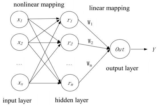
Figure 5.
RBF neural network structure diagram.
The basic principle of RBF neural network is to map the linearly inseparable sample of low-dimensional space to high-dimensional hidden layer space without using weight connection and make the high-dimensional space become linearly separable [55]. The mapping between the hidden layer and the output space is linear. In other words, the network output is the linear weighted sum of the hidden unit output. It can be seen that the network output is linear with respect to tunable arguments, so that the network weight can be resolved directly from the system of linear equations, thus greatly accelerating the learning speed and preventing local minimum problem.
Assume that RBF neural network input is X = {x1, x2, …, xn} (where X∈Rn), thus, the hidden layer output Zj, can be obtained using Equation (6):
where, Rj () is the RBF, and Cj is the center of the jth basis function.
Generally, Rj is set as the n-dimensional Gaussian kernel function, as shown in Equation (7).
where, is the square of the width of the jth basis function.
Through the linear correlation between hidden layer and output layer, the output of RBF neural network Y can be obtained using Equation (8).
where, Wj is the weight between hidden layer and output layer of RBF neural network; and m is the number of hidden layers.
Additionally, the sum of the differences between the actual output and the expectation of the RBF neural network is utilized as the fitness function in the PSO algorithm, as shown in Equation (9).
where, n is the iterations; Di is the expected value in the ith iteration; and Yi is the actual output of the RBF neural network in the ith iteration. The lower the Fit value, the better the optimization effect.
At present, the RBF neural network has caught scholars’ attention in many fields due to its simple structure and excellent approximation characteristics. It is mostly applied in classification mode [56], data mining [57] and other fields [58,59,60]. Compared with the BP neural network, the RBF neural network has better generalization ability and stronger global approximation to nonlinear functions. In addition, the RBF neural network has fast learning speed and the ability to avoid local extremum. Therefore, in this paper, RBF neural network is utilized to construct the thermal error model for the spindle of CNC machine tool.
4.2.2. The Improved PSO Algorithm
The PSO algorithm was first proposed by Eberhart and Kennedy in 1995 [61]. Each particle in the algorithm signifies a probable solution to the problem. Through the interaction of individual behavior and group information, the purpose of solving the problem is achieved.
Particles are initialized in the search space during the process of solving. They are defined by velocity, position, and fitness value. The fitness value that represents the quality of particles can be calculated by means of fitness function. The position of particles in space updates with the individual extremum pbest (the best individual position) and population extremum gbest (the best population position). Each time the particles update, the fitness values are re-calculated, which result in the update of pbest and gbest.
Moreover, the trajectory of particles is influenced by learning factors c1 and c2 which represent the weight of the statistical direction of acceleration of each particle towards pbest and gbest, respectively. If c1 takes a larger value, particles will wander in the local range. Otherwise, particles will converge prematurely and lead to local extremum. To effectively control the velocity of particles, a compression factor is introduced to make the PSO algorithm balance between global and local search.
The velocity vij and position xij (where i is the iteration and j is the number of variables) of particles can be calculated using the following Equation:
where, r1 and r2 are random numbers distributed between [0, 1]; c1 and c2 are non-negative constants; t is the iterations; and φ is the compression factor.
4.2.3. IPSO-RBFNN Model on Thermal Error Modeling
With the temperature-sensitive variables chosen using the KR-BPNN method, the IPSO-RBFNN model is further utilized to fit the data.
The construction process of the IPSO-RBFNN model is as follows:
Step 1: Initializing parameters and weights of RBF neural network;
Step 2: Establishing the thermal error model for the spindle of CNC machine tool based on RBF neural network, and taking the sum of differences between actual output and expectation value as the fitness function of the particle swarm;
Step 3: Updating parameters and weight using the improved PSO algorithm, as well as the velocity and position of particles;
Step 4: Determining whether to end conditions (iteration). If yes, getting the optimal arguments of the RBF neural network; otherwise, repeating step 3.
The flow of IPSO-RBFNN model on thermal error modeling is shown in Figure 6.
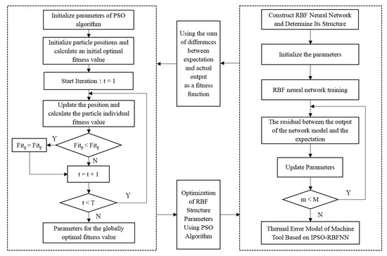
Figure 6.
Flow chart of establishing thermal error model based on IPSO-RBFNN.
5. Performance Evaluation
The choose results of temperature-sensitive variables set through the KR-BPNN method are provided in Section 5.1 The prediction performance analysis of the IPOS-RBFNN model of thermal errors is presented in Section 5.2.
5.1. Temperature-Sensitive Variables Selection
Prior to establishing the thermal error prediction model, the temperature-sensitive variables were chosen based on the experimental data at 12,000 rpm. Sixteen temperature transducers were arranged in five different heat source regions in the experiment.
According to the KR-BPNN method, different K values will produce different clusters. Considering that there are five thermal source regions, and both the ambient temperature transducer and the spindle region transducer are essential, the K value is set between [3, 8]. Seventy percent of the experimental data are utilized to train the model, and the remaining sample data are used to test the model.
Based on Equations (3) and (4), the absolute mean correlation coefficient is obtained, as shown in Table 3.
Table 3.
Absolute mean correlation coefficient between temperature variables and thermal errors.
Table 4 shows the clustering results of different K values, and the temperature-sensitive variables sets under different K values are shown in Table 5.
Table 4.
Clustering results of different K values.
Table 5.
Sets of temperature-sensitive variables under different K values.
The set of temperature variables under different K values is used as the temperature input of the BP neural network to setup the thermal error model. The predictive performance of the model is evaluated according to Equation (5), and the results are shown in Figure 7.
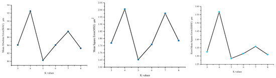
Figure 7.
Evaluation result under different K values.
It can be seen from Figure 7 that the values of MAE, MSE, and RMSE are all smallest when K = 5. Obviously, the BP neural network established by the combination of sensitive temperature points corresponding to K = 5 has the best prediction performance. Hence, the combination of sensitive temperature points {T1, T6, T9, T13, T16} is determined as the combination of sensitive temperature points of the overall machine tool.
5.2. Performance Comparison
To verify the optimization of RBF neural network by the improved PSO algorithm with compression factor, different neural networks are constructed for comparative analysis. Figure 8 is a graph comparing the relationship between the fitness value and the iterations of improved PSO and PSO. It is obvious that on the premise of the same iterations, the RBF neural network based on improved PSO algorithm has better fitness results, and it also needs fewer iterations under the same fitness value. Hence, it is proved that the improved PSO algorithm has better optimization precision and faster convergence speed than the PSO algorithm.
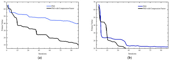
Figure 8.
Comparison between PSO and IPSO. (a) The same iterations; (b) The same fitness value.
To evaluate the prediction performance of the IPSO-RBFNN model and compare it to different algorithms, three evaluation metrics are computed, including deformation, residual error, and mean residual error.
The Z direction deformations of different algorithms, including RBF neural network (RBFNN), BP neural network (BPNN), PSO-BPNN, PSO-RBFNN, and IPSO-RBFNN based on the experimental data at 12,000 rpm are shown in Figure 9.
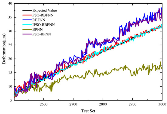
Figure 9.
Z direction deformations of different algorithms.
It can be seen that the predicting deformations of IPSO-RBFNN and PSO-RBFNN are fitted better for the expected value.
To compare the prediction performance of above algorithms further, the residual error and mean residual error are computed, and the results are displayed in Figure 10.
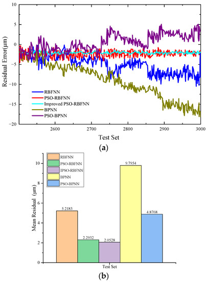
Figure 10.
Prediction performance of each model. (a) Residual error; (b) Mean residual error.
It is apparent that the residual errors of IPSO-RBFNN and PSO-RBFNN are smaller than other algorithms. Furthermore, Figure 10 indicates that the mean residual error of IPSO-RBFNN is smallest among all the algorithms.
The above analysis shows that, the predictive performance of IPSO-RBFNN is better than PSO-RBFNN. As a result, compared with PSO-RBFNN, the mean residual error of IPSO-RBFNN is reduced by 10.48%.
6. Experimental Verification
In this section, the predictive performance of IPSO-RBFNN model is verified based on different experimental conditions to reflect the robustness of the model. In Section 6.1, the prediction results of thermal error in Z direction based on IPSO-RBFNN model at different rotational velocities are analyzed. In Section 6.2, the predicted results of more thermal error terms based on the IPSO-RBFNN model are analyzed.
6.1. Verification of the IPSO-RBFNN Model at Different Rotational Velocities
Based on the trained neural network model, the verification experiment is carried out. The experimental data at 4000 rpm and 8000 rpm are used to analyze the prediction performance of the thermal error of the spindle in Z-direction based on IPSO-RBFNN. The thermal errors in Z-direction at 4000 rpm and 8000 rpm are shown in Figure 11 and Figure 12, respectively.
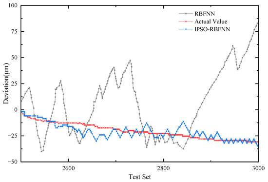
Figure 11.
The thermal errors in Z-direction of different models at 4000 rpm.
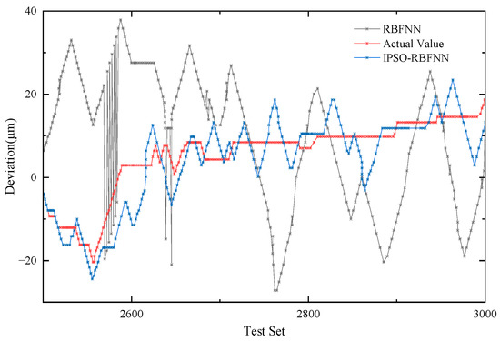
Figure 12.
The thermal errors in Z-direction of different models at 8000 rpm.
Figure 11 and Figure 12 show that the predicted values at 4000 rpm and 8000 rpm based on the IPOS-RBFNN model are both closer to the actual values than the RBFNN model. Furthermore, two metrics, MSE and RMSE, are used to evaluate the predictive performance of IPOS-RBFNN and RBFNN models. The results are displayed in Table 6. It is visible from the table that the RMSE and MSE values of IPOS-RBFNN model are both much smaller than those of RBFNN model at 4000 rpm and 8000 rpm, which proves that IPOS-RBFNN model has higher predictive accuracy than RBFNN model.
Table 6.
Evaluation results of predictive performance of two models.
6.2. Verification of the IPSO-RBFNN Models with Different Error Terms
In Section 5.2 and Section 6.1, the predictive performance of thermal error in Z direction based on the IPSO-RBFNN model has been analyzed at different velocities. In this section, the prediction performance of thermal errors in X2 and Y1 direction at 800 rpm will be verified. The thermal errors in X2 and Y1 direction at 800 rpm are shown in Figure 13 and Figure 14, respectively.
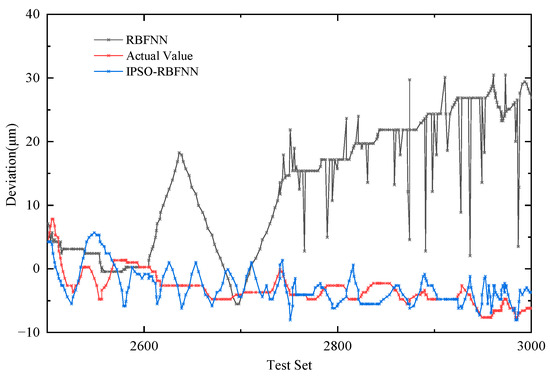
Figure 13.
Verification results of X2 error term of two models at 800 rpm.
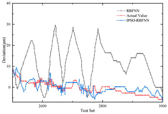
Figure 14.
Verification results of Y1 error term of two models at 800 rpm.
Figure 13 and Figure 14 show that the predicted values of the thermal error in X2 and Y1 direction at 800 rpm based on the IPOS-RBFNN model are both closer to the actual values than the RBFNN model. In the same way, two metrics, MSE and RMSE, are used to evaluate the predictive performance of the models.
It is visible from Table 7 that the RMSE and MSE values of IPOS-RBFNN model are both much smaller than those of RBFNN model, both in X2 direction or Y1 direction, which proves that the IPOS-RBFNN model has a higher predictive accuracy than the RBFNN model.
Table 7.
Evaluation of the prediction results of the two models.
7. Conclusions
In this article, an improved model which combines the K-means clustering algorithm and correlation analysis method based on BPNN, named as the KR-BPNN method, is proposed to choose the temperature-sensitive variables. Further, the IPSO-RBFNN model is utilized to predict the thermal errors for the spindle of CNC machine tool on the basis of the chosen temperature-sensitive variables. Since the IPSO-RBFNN model is established based on the improved PSO algorithm by introducing a compression factor to make the PSO algorithm balance between global and local search, it allows to optimize the structure arguments of RBFNN so as to promote the predictive accuracy of thermal error model for the spindle. On the foundation of the experimental data on the CNC machine tool, named DMG-DMU65, the predictive accuracy of IPSO-RBFNN model in Z direction reaches 2.05 μm. Compared with other methods, it is improved by at least 10.48%, which means it is remarkably better than the other four current neural network methods. The experiment verification shows that the proposed model has good predictive accuracy for different thermal error terms at different velocities, indicating that the model has strong robustness to a certain extent.
Further research is needed in several important directions. Firstly, the PSO algorithm with compression factor was used to optimize the RBF parameters in this paper, but introducing more advanced parameter optimization methods is worth studying. Secondly, during the experiment, the spindle was loaded only with an elastic tool handle and a standard test bar, so its predictive performance in the actual cutting scenario needs to be further verified. Finally, the thermal error compensation experiment based on the prediction model needs further research.
Author Contributions
Conceptualization and writing—review and editing, Z.F.; Methodology and writing—original draft preparation, X.M.; validation, W.J. and F.S.; investigation and data curation, X.L. All authors have read and agreed to the published version of the manuscript.
Funding
This research was funded by the Key Science and Technology Research Projects of Sichuan Province, grant number 2021ZHCG0015, the Ministry of Education “Chunhui” Plan of China, grant number Z2017074, and the Artificial Intelligence Key Laboratory of Sichuan Province, grant number 2022RYY02.
Institutional Review Board Statement
Not applicable.
Informed Consent Statement
Not applicable.
Data Availability Statement
Not applicable.
Acknowledgments
The authors specially thank Shuai Zhao and XiangZhi Chen for their support of experimental works.
Conflicts of Interest
The authors declare no conflict of interest.
References
- Mancisidor, I.; Zatarain, M.; Munoa, J.; Dombovari, Z. Fixed Boundaries Receptance Coupling Substructure Analysis for Tool Point Dynamics Prediction. Adv. Mater. Res. 2011, 223, 622–631. [Google Scholar] [CrossRef]
- Ramesh, R.; Mannan, M.; Poo, A. Error compensation in machine tools—A review Part I: Geometric, cutting-force induced and fixture-dependent errors. Int. J. Mach. Tools Manuf. Des. Res. Appl. 2000, 40, 1235–1256. [Google Scholar] [CrossRef]
- Abele, E.; Altintas, Y.; Brecher, C. Machine tool spindle units. Cirp. Ann. 2010, 59, 781–802. [Google Scholar] [CrossRef]
- Pan, S.W. Summary of Research Status on Thermal Error Robust Modeling of NC Lathe. Tool Eng. 2007, 41, 10–14. [Google Scholar]
- Ni, J. CNC machine accuracy enhancement through real-time error compensation. Manuf. Sci. Eng. 1997, 119, 717–725. [Google Scholar] [CrossRef]
- Liu, J.; Ma, C.; Wang, S. Precision loss modeling method of ball screw pair. Mech. Syst. Signal Process. 2020, 135, 106397. [Google Scholar] [CrossRef]
- Grama, S.N.; Mathur, A.; Badhe, A.N. A model-based cooling strategy for motorized spindle to reduce thermal errors. Int. J. Mach. Tools Manuf. 2018, 132, 3–16. [Google Scholar] [CrossRef]
- Chen, T.-C.; Chang, C.-J.; Hung, J.-P.; Lee, R.-M.; Wang, C.-C. Real-Time Compensation for Thermal Errors of the Milling Machine. Appl. Sci. 2016, 6, 101. [Google Scholar] [CrossRef]
- Aguirre, G.; Nanclares, A.; Urreta, H. Thermal Error Compensation for Large Heavy Duty Milling-Boring Machines. In Proceedings of the Euspen Special Interest Group Meeting, Thermal Issues, Zurich, Switzerland, 7 March 2014; pp. 19–20. [Google Scholar]
- Ivo, P.; Dagmar, B. Total Least Squares Approach to Modeling: A Matlab Toolbox. Acta Montan. Slovaca 2010, 15, 158. [Google Scholar]
- Wang, H.; Li, T.; Wang, L.; Li, F. Review on Thermal Error Modeling of Machine Tools. J. Mech. Eng. 2015, 51, 119–128. [Google Scholar] [CrossRef]
- Li, Y.; Yu, M.; Bai, Y.; Hou, Z.; Wu, W. A Review of Thermal Error Modeling Methods for Machine Tools. Appl. Sci. 2021, 11, 5216. [Google Scholar] [CrossRef]
- Li, Y.; Zhao, W.; Lan, S.; Ni, J.; Wu, W.; Lu, B. A review on spindle thermal error compensation in machine Tools. Int. J. Mach. Tools Manuf. 2015, 95, 20–38. [Google Scholar] [CrossRef]
- Ramesh, R.; Mannan, M.A.; Poo, A.N.; Keerthi, S.S. Thermal error measurement and modelling in machine tools. Part II. Hybrid Bayesian Network—Support vector machine model. Int. J. Mach. Tools Manuf. 2003, 43, 405–419. [Google Scholar] [CrossRef]
- Wang, C.N.; Qin, B.; Qin, Y.; Yuan, Y.; Wu, Q.C.; Zhang, W.X. Thermal Error Prediction of Numerical Control Machine Based on Improved Particle Swarm Optimized Back Propagation Neural Network. In Proceedings of the 11th International Conference on Natural Computation (ICNC), Zhangjiajie, China, 15–17 August 2015; pp. 820–824. [Google Scholar]
- Liu, K.; Yu, L.; Yang, D.Z. Comparative Experimental Research on Modeling of Thermal Error Neural Network of Machine Tool. J. Sichuan Univ. Sci. Eng. Nat. Sci. Ed. 2018, 31, 21–26. [Google Scholar]
- Ren, M.; Huang, X.; Zhu, X.; Shao, L. Optimized PSO algorithm based on the simplicial algorithm of fixed point theory. Appl. Intell. 2020, 50, 2009–2024. [Google Scholar] [CrossRef]
- Ghasemi, M.; Akbari, E.; Rahimnejad, A.; Razavi, S.; Ghavidel, S.; Li, L. Phasor particle swarm optimization: A simple and efficient variant of PSO. Soft Comput. A Fusion Found. Methodol. Appl. 2019, 23, 9701–9718. [Google Scholar] [CrossRef]
- Hojung, L.; Cho-Jui, H.; Jong-Seok, L. Local Critic Training for Model-Parallel Learning of Deep Neural Networks. IEEE Trans. Neural Netw. Learn. Syst. 2021, 33, 1–13. [Google Scholar]
- Kostenko, V.A.; Seleznev, L.E. Random Search Algorithm with Self-Learning for Neural Network Training. Opt. Mem. Neural Netw. 2021, 30, 180–186. [Google Scholar] [CrossRef]
- Bin, W.; Lan, Y.; Feng, W.; Diyi, C. Fuzzy predictive functional control of a class of non-linear systems. IET Control Theory Appl. 2019, 13, 2281–2288. [Google Scholar]
- Seyed, M.; Aliakbar, J. Fuzzy tracking control of fuzzy linear dynamical systems. ISA Trans. 2020, 97, 102–115. [Google Scholar]
- Iyer, V.H.; Mahesh, S.; Malpani, R.; Sapre, M.; Kulkarni, A.J. Adaptive Range Genetic Algorithm: A hybrid optimization approach and its application in the design and economic optimization of Shell-and-Tube Heat Exchanger. Eng. Appl. Artif. Intell. Int. J. Intell. Real-Time Autom. 2019, 85, 444–461. [Google Scholar] [CrossRef]
- Zhang, D.; Li, W.; Wu, X.; Lv, X. Application of simulated annealing genetic algorithm-optimized back propagation (BP) neural network in fault diagnosis. Int. J. Model. Simul. Sci. Comput. 2019, 10, 1950024.1–1950024.12. [Google Scholar] [CrossRef]
- Zhu, Y.; Zhou, L.; Xu, H. Application of improved genetic algorithm in ultrasonic location of transformer partial discharge. Neural Comput. Appl. 2020, 32, 1755–1764. [Google Scholar] [CrossRef]
- Li, Z.; Yang, J.; Fan, K.; Zhang, Y. Integrated geometric and thermal error modeling and compensation for vertical machining centers. Int. J. Adv. Manuf. Technol. 2015, 76, 1139–1150. [Google Scholar] [CrossRef]
- Mayr, J.; Blaser, P.; Ryser, A.; Hernández-Becerro, P. An adaptive self-learning compensation approach for thermal errors on 5-axis machine tools handling an arbitrary set of sample rates. CIRP Ann. 2018, 67, 551–554. [Google Scholar] [CrossRef]
- Liu, H.W.; Yang, Y.; Xiang, H.; Wang, J.P.; Chen, G.H. Research on Thermal Error Compensation Technology of Machine Tool Spindle On Least Square Method. Mach. Des. Res. 2020, 36, 130–133. [Google Scholar]
- Pajor, M.; Zapłata, J. Compensation of thermal deformations of the feed screw in a CNC machine tool. Adv. Manuf. Sci. Technol. 2011, 35, 9–17. [Google Scholar]
- Liu, P.; Du, Z.; Li, H.; Deng, M.; Feng, X.; Yang, J. Thermal error modeling based on BiLSTM deep learning for CNC machine tool. Adv. Manuf. 2021, 9, 235–249. [Google Scholar] [CrossRef]
- Shi, H.; Xiao, X.; Mei, X.; Tao, T.; Wang, H. Thermal error modeling of machine tool based on dimensional error of machined parts in automatic production line. ISA Trans. 2022, 135, 575–584. [Google Scholar] [CrossRef]
- Jiang, H.; Yang, J.G. Application of an Optimized Grey System Model on 5-Axis CNC Machine Tool Thermal Error Modeling. In Proceedings of the 2010 International Conference on E-Product E-Service and E-Entertainment, Henan, China, 7–9 November 2010; pp. 1–5. [Google Scholar]
- Tien, T.-L. A research on the grey prediction model GM(1,n). Appl. Math. Comput. 2012, 218, 4903–4916. [Google Scholar] [CrossRef]
- Wang, S.; Hu, S.W.; Jiang, X.L.; Xu, F.; Wu, J. Thermal Error Modeling Optimization Method for Numerical Control Machine Tool Based on CS—GMC (1,N). Mach. Tool Hydraul. 2020, 48, 126–131. [Google Scholar]
- Miao, E.M.; Gong, Y.Y.; Cheng, T.J.; Chen, H.L. Application of support vector regression machine to thermal error modelling of machine tools. Opt. Precis. Eng. 2013, 21, 980–986. [Google Scholar] [CrossRef]
- Zhang, E.Z.; Qi, Y.L.; Ji, S.J.; Chen, Y.P. Thermal Error Modeling and Compensation for Precision Polishing Platform Based on Support Vector Regression Machine. Modul. Mach. Tool Autom. Manuf. Tech. 2017, 58, 48–51. [Google Scholar] [CrossRef]
- Li, Z.; Wang, Q.; Zhu, B.; Wang, B.; Zhu, W.; Dai, Y. Thermal error modeling of high-speed electric spindle based on Aquila Optimizer optimized least squares support vector machine. Case Stud. Therm. Eng. 2022, 39, 102432. [Google Scholar] [CrossRef]
- Huang, Y.; Zhang, J.; Li, X.; Tian, L. Thermal error modeling by integrating GA and BP algorithms for the high-speed spindle. Int. J. Adv. Manuf. Technol. 2014, 71, 1669–1675. [Google Scholar] [CrossRef]
- Liu, H.; Miao, E.M.; Feng, D.; Li, J.G.; Ma, H.F.; Zhang, Z.H. Thermal Error Modeling Algorithm Based on Overall Adjustment Strategy Neural Network. J. Chongqing Univ. Technol. Nat. Sci. 2020, 34, 107–115. [Google Scholar]
- Su, T.M.; Ye, S.P.; Sun, W. Thermal Error Compensation Modeling Based on Fuzzy C -means Clustering Algorithm and RBF Neural Network Modeling. Modul. Mach. Tool Autom. Manuf. Tech. 2011, 10, 1–4. [Google Scholar]
- Zhang, H.N. Research on Modeling of Machining Center Spindle Thermal Error Based on Improved RBF Network. Technol. Autom. Appl. 2019, 38, 60–74. [Google Scholar]
- Elghaish, F.; Talebi, S.; Abdellatef, E.; Matarneh, S.T.; Hosseini, M.R.; Wu, S.; Mayouf, M.; Hajirasouli, A.; Nguyen, T.Q. Developing a new deep learning CNN model to detect and classify highway cracks. J. Eng. Des. Technol. 2022, 20, 993–1014. [Google Scholar] [CrossRef]
- Asifullah, K.; Anabia, S.; Umme, Z.; Aqsa, S. A survey of the recent architectures of deep convolutional neural networks. Artif. Intell. Rev. 2020, 53, 5455–5516. [Google Scholar]
- Wang, R.; Lei, Z.; Zhang, Z.; Gao, S. Dendritic Convolutional Neural Network. IEEJ Trans. Electr. Electron. Eng. 2022, 17, 302–304. [Google Scholar] [CrossRef]
- Aziz, R.M.; Mahto, R.; Goel, K.; Das, A.; Kumar, P.; Saxena, A. Modified Genetic Algorithm with Deep Learning for Fraud Transactions of Ethereum Smart Contract. Appl. Sci. 2023, 13, 697. [Google Scholar] [CrossRef]
- Rezaei, H.; Faaljou, H.; Mansourfar, G. Stock price prediction using deep learning and frequency decomposition. Expert Syst. Appl. 2021, 169, 114–332. [Google Scholar] [CrossRef]
- Yin, X.; Tao, X. Prediction of Merchandise Sales on E-Commerce Platforms Based on Data Mining and Deep Learning. Sci. Program. 2021, 2021, 2179692. [Google Scholar] [CrossRef]
- Wang, S.; Cao, J.; Yu, P. Deep Learning for Spatio-Temporal Data Mining: A Survey. IEEE Trans. Knowl. Data Eng. 2020, 1, 3681–3700. [Google Scholar] [CrossRef]
- Wu, C.; Xiang, S.; Xiang, W. Spindle thermal error prediction approach based on thermal infrared images: A deep learning method. J. Manuf. Syst. 2021, 59, 67–80. [Google Scholar]
- ISO 230-3; Test Code for Machine Tools Part 3: Determination of Thermal Effects 2020. ISO Copyright Office: London, UK, 2020.
- MacQueen, J. Some methods for classification and analysis of multivariate observations. Symp. Math. Stat. Probab. 1967, 281–297. [Google Scholar]
- Kristina, P.; Sinaga; Ishtiaq, H.; Miin-Shen, Y. Entropy K-Means Clustering with Feature Reduction under Unknown Number of Clusters. IEEE Access 2021, 9, 67736–67751. [Google Scholar]
- Yuan, Q.; Ma, C.; Liu, J.; Gui, H.; Li, M.; Wang, S. Correlation analysis-based thermal error control with ITSA-GRU-A model and cloud-edge-physical collaboration framework. Adv. Eng. Inform. 2022, 54, 101759. [Google Scholar] [CrossRef]
- Wei, J.; Xu, S.; Liu, H. Simplified Model for Predicting Fabric Thermal Resistance According to its Microstructural Parameters. Fibres Text. East. Eur. 2015, 23, 57–60. [Google Scholar]
- Ma, C.; Zhao, L.; Mei, X.; Shi, H.; Yang, J. Thermal error compensation of high-speed spindle system based on a modified BP neural network. Int. J. Adv. Manuf. Technol. 2017, 89, 3071–3085. [Google Scholar] [CrossRef]
- Jia, W.; Zhao, D.; Ding, L. An optimized RBF neural network algorithm based on partial least squares and genetic algorithm for classification of small sample. Appl. Soft Comput. 2016, 48, 373–384. [Google Scholar] [CrossRef]
- Qin, Z.; Chen, J.; Liu, Y.; Lu, J. Evolving RBF Neural Networks for Pattern Classification. Lect. Notes Comput. Sci. 2005, 3801, 957–964. [Google Scholar]
- Markus, B.; Oliver, B.; Timo, H.; Ralf, K.; Bernhard, S.; Robert, W. Technical data mining with evolutionary radial basis function classifiers. Appl. Soft Comput. 2009, 9, 765–774. [Google Scholar]
- Hasan, Ö.; Yiğit, A.; Mert, Ş.; Abdullah, K. Estimations for (n,α) reaction cross sections at around 14.5MeV using Levenberg-Marquardt algorithm-based artificial neural network. Appl. Radiat. Isot. 2022, 192, 110609. [Google Scholar]
- Akkoyun, S. Estimation of fusion reaction cross-sections by artificial neural networks. Nucl. Instrum. Methods Phys. Res. Sect. B 2020, 462, 51–54. [Google Scholar] [CrossRef]
- Kennedy, J.; Eberhart, R. Particle Swarm Optimization. In Proceedings of the ICNN’95—International Conference on Neural Networks, Perth, WA, Australia, 27 November–1 December 1995. [Google Scholar]


Disclaimer/Publisher’s Note: The statements, opinions and data contained in all publications are solely those of the individual author(s) and contributor(s) and not of MDPI and/or the editor(s). MDPI and/or the editor(s) disclaim responsibility for any injury to people or property resulting from any ideas, methods, instructions or products referred to in the content. |
© 2023 by the authors. Licensee MDPI, Basel, Switzerland. This article is an open access article distributed under the terms and conditions of the Creative Commons Attribution (CC BY) license (https://creativecommons.org/licenses/by/4.0/).