Abstract
Light detection and ranging (LiDAR) has been applied in many areas because of its excellent performance. An easily achievable, cost-effective, and high-performance ranging method is a major challenge of LiDAR. Meanwhile, with the increasing applications of LiDAR, numerous LiDARs can be made to operate simultaneously, and potential interference is inevitable. Therefore, immunity against interference is paramount in LiDAR systems. In this paper, we demonstrated a ranging method referred to as phase-modulated continuous-wave (PhMCW). A detection range of 50 m and a ranging error of 2.2 cm are achieved. A one-dimensional scanning LiDAR system that is capable of detecting targets at 28 m is built, demonstrating the validation of the PhMCW method. Moreover, we propose a quantitative method for evaluating the anti-interference capability of lidar systems. The p-values of the Ljung–Box test were 0.0589 and 0.6327 for ToF and coherent LiDAR interferences, respectively, indicating that the PhMCW system is immune to interference. The proposed method can be applied to all types of LiDAR systems, regardless of the ranging method or beam-steering technique used.
1. Introduction
Light detection and ranging (LiDAR) has garnered considerable attention because of its excellent performance [1,2,3,4,5,6,7,8,9,10]. Compared to its counterpart operating at radio frequencies, LiDAR can achieve long-range, superior accuracy and angular resolution owing to the short wavelength of light [1]. LiDAR devices have been applied in many areas such as autonomous vehicles, robotics, and drones. In particular, autonomous vehicle technology requires an eye-safe, anti-interference, and low-cost ranging method.
The ranging mechanism is a core technology of the LiDAR system [11], and the time-of-flight (ToF) ranging method based on pulsed light has been the dominant technology in commercial lidar applications because of its simplicity and ease of implementation [2,5,12,13,14,15]. However, the detection range of the ToF is primarily limited by eye safety issues [16]. In addition, to improve the precision of the lidar system to the millimeter scale, the modulation bandwidth must be at the GHz level [6,17]. Such high-level modulation devices are difficult to use in commercial applications. Therefore, much research interest has moved on to frequency-modulated continuous waves (FMCW) [7,18,19,20]. However, FMCW is plagued by low stability, high complexity, and high insertion loss of the frequency modulation source [21,22,23,24]. Consequently, the use of FMCW is impractical for commercial applications. Thus, LiDAR requires an easily achievable, cost-effective, high-performance ranging method.
Moreover, in realistic applications, LiDAR systems are encountering situations wherein numerous LiDARs operate simultaneously and a potential interference is inevitable [25,26,27]. Therefore, immunity against interference is paramount in LiDAR systems [26]. However, the ToF is notorious for its lack of anti-interference capability [12,15,26]. Several studies have focused on the modification of sensors in ToF ranging systems. Lee et al. [28] used an internal interference light reduction structure on the sensors to reduce the measurement error. Dashpute et al. [29] used the polarization state of reflected light to reduce the depth measurement error. Moreover, to improve the capability of interference by design, the authors of [25,30,31] analyzed different interference modes by modeling the signal interference. However, the problem of being easily interfered with is prevalent in ToF LiDARs. Thus, there is a need for a new ranging method with a much better anti-interference capability than ToF.
Meanwhile, in many evaluations of LiDAR’s anti-interference capability, the victim LiDAR is placed in an indirect interference environment. Carballo et al. [32] performed measurements from a fixed position using multiple LiDARs mounted side-by-side and operated them simultaneously. Popko et al. [31] used a scanner at different angles to modify direct and scattered interference. However, in these reports, the victim and interferential LiDARs were not synchronized in either the time domain or the field of view, implying that the possibility of disturbance caused to the victim LiDAR remains completely uncertain and random. Therefore, the evaluation results were not convincing. To quantitatively analyze the anti-interference capability of LiDARs, a novel test method is required. As for the FMCW, although the coherent ranging method has an intrinsic rejection of interference [19], to the best of our knowledge, there have been no experimental demonstrations.
In this study, we demonstrated a ranging method referred to as phase-modulated continuous-wave (PhMCW), which exhibited excellent anti-interference capabilities. First, we proposed a PhMCW ranging mechanism and combined it to set up a ranging system. In addition, we varied the distance of a diffusive reflection board placed at the furthest distance of 50 m, and the ranging error was as low as 2.2 cm. A one-dimensional scanning LiDAR system that is capable of detecting targets at 28 m was built, demonstrating the validation of the PhMCW method. Moreover, we proposed a modified model for ranging precision. Furthermore, using the PhMCW as an example, we proposed two sets of anti-interference capability experiments against ToF and coherent LiDARs. Through an analysis of the differences in the measured precision with and without interference through the Ljung–Box method, we arrived at a quantitative conclusion about the anti-interference capability of LiDARs. The p-values of the PhMCW system were 0.0589 and 0.6327 with ToF and coherent LiDAR interference, respectively, demonstrating the excellent capability of the PhMCW against interference. Moreover, the proposed method can be applied to all types of lidar systems. To the best of our knowledge, this is the first quantitative method to evaluate the anti-interference capability of LiDARs.
2. PhMCW Mechanism
The mechanism of PhMCW is briefly illustrated in Figure 1a. The laser phase is modulated by a rectangular waveform, where is the initial optical phase, is modulation depth, is an integer, and is the period of phase modulation.
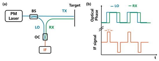
Figure 1.
(a) A schematic of the PhMCW system. PM: phase modulation; BS: beam splitter and OC: optical coupler. (b) The optical phase of the LO and RX and the waveform of the IF signal.
The modulated laser is coupled as a local oscillator (LO) and transmitter signal (TX), which is transmitted into free space. The TX signal will be back-scattered by the target and collected by the receiver. Subsequentially, the received signal (RX) and LO are mixed to obtain an intermediate frequency (IF) signal. For a stationary target, ignoring the DC term of the IF signal, it can be expressed as:
where is the amplitude of the electric field of LO, is the amplitude of the electric field of RX, is the optical frequency, and is the time of flight. As shown in Figure 1b, the IF signal consists of a bunch of pulses whose pulse width is equal to . Therefore, by measuring the pulse width of the IF signal and then multiplying it by , where is the speed of light, we can obtain the distance information.
3. Ranging Experiments
According to the mechanism, we built a PhMCW system based on a monostatic configuration to demonstrate the validation of the proposed PhMCW method, as shown in Figure 2. We chose a 1550 nm CW narrow-linewidth laser (Connect CoSF-D) as the light source, followed by an erbium-doped fiber amplifier. The optical phase is modulated by a LiNbO3 phase modulator, which is driven by an arbitrary function generator (AFG). After that, the modulated laser is split into LO and TX by a 10:90 beam splitter, and the TX signal is collimated and emitted into free space. The RX signal, back-scattered by the target, is routed to a 2 × 2 optical coupler and mixed with the LO signal. The mixed optical signal is received by a pair of balanced photodetectors (Thorlabs PDB470C-AC) and transmitted to the electrical IF signal. Finally, the IF signal is monitored, stored, and digitally processed by an oscilloscope (Tektronix MSO54). We chose an off-the-shelf diffused reflection board with a reflectivity of 90% as the target, and the distance to the target was varied from 5 m to a maximum of 50 m.
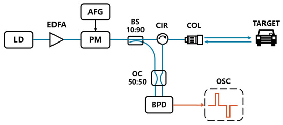
Figure 2.
A schematic of the PhMCW system. LD: laser; EDFA: erbium-doped fiber amplifier; PM: phase modulator; AFG: arbitrary function generator; OC: optical coupler; CIR: circulator; COL: collimator; BPD: balance photodetector; and OSC: oscilloscope.
At each distance, we performed 50 ranging measurements, and the averaged results are shown in Figure 3. The linear relationship between the measured distance and the actual distance indicates the validation of the PhMCW method and the ranging error is as low as 2.2 cm, suggesting good accuracy.
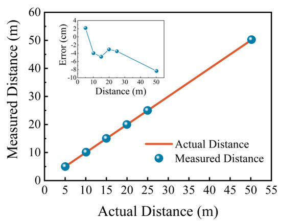
Figure 3.
Measured distance as a function of actual distance. Inset is the ranging errors of each distance.
In addition to accuracy, precision is another important criterion for LiDAR [1,11,12,18]. Therefore, we calculated the measured results with varying distances, and the distribution results are shown in Figure 4, where the dashed curves indicate Gaussian fits and all distributions confirm a Gaussian distribution. The minimum and maximum standard deviations were 1.7 and 6.2 cm, respectively, demonstrating the exceptional precision of the PhMCW system.
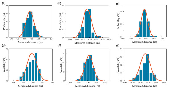
Figure 4.
(a–f) Distribution figures of the ranging results at actual distances of 5.025 m, 10.09 m, 14.99 m, 19.96 m, 24.983 m, 50.179 m, respectively. Orange lines indicate Gaussian fits.
Theoretically, the ranging precision is inversely proportional to the square root of the signal-to-noise ratio (SNR), that is, [33]. In our ranging system, the power of the LO was several orders of magnitude higher than that of the RX. Therefore, the noise in the system is believed to be dominated by the shot noise of the LO. Meanwhile, the IF signal level is proportional to the amplitude of the electric field of the RX signal , that is, to the square root of the RX power . According to the LiDAR link budget, is primarily affected by the target reflectivity and the distance to the target [19]. Therefore, is derived to be proportional to and inversely proportional to , as given by . The target reflectivity is 90%, and, as a result, the ranging precision can be expressed as , where is a coefficient. Figure 5 illustrates the precision values extracted from Figure 4. The precision formulas fitted from Figure 5 are . According to such a model, a target located at 100 m would result in a precision of 8.93 cm, which is comparable to commercial LiDARs [32], suggesting promising application prospects for the PhMCW method.
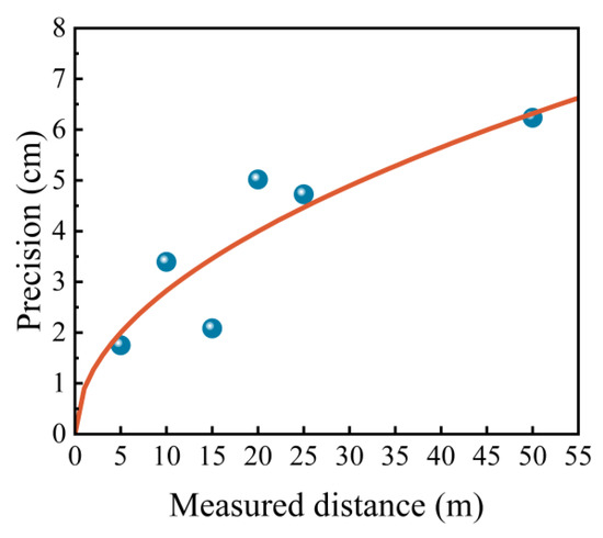
Figure 5.
Precision as a function of the measured distance. The orange line indicates the 1/2-power polynomial fitting.
In order to demonstrate the validation of the PhMCW ranging method, we built a PhMCW LiDAR by mounting the collimator, shown in Figure 2, on a rotational base, and the laser beam direction is mechanically steered horizontally. Due to the narrow width of the clean room’s corridor, the scanning angle is thus varied from −2° to −2° with a step of 0.5°. Figure 6a gives a picture of the experimental scene, showing targets consisting of a diffused reflection board, laboratory doors, and a researcher at approximate distances of 15 m, 28 m, and 5 m, respectively. The measured results are shown in Figure 6b for average target distances of 15.13 m, 27.85 m, and 5.03 m, respectively. The measured distances are in good agreement with the actual distances.
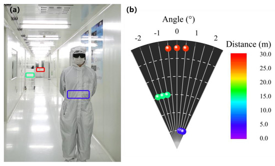
Figure 6.
One-dimensional scanning results. (a) An image of the experimental scene. The colored boxes indicate the corresponding measurement positions. (b) The measured results of targets. The points are color-coded by the distance values.
4. Anti-Interference Capability
With the increasing applications of LiDAR, numerous LiDARs can be made to operate simultaneously, and potential interference is inevitable. For autonomous vehicles, the anti-interference capability is among the most important issues owing to safety requirements [26]. Therefore, exploring the anti-interference capabilities of LiDAR systems is crucial. By measuring the anti-interference capability of the PhMCW, we demonstrated two sets of experiments that can quantitatively analyze the anti-interference capability, which can be used in any other LiDAR system.
The setup of an anti-interference experiment against ToF is illustrated in Figure 7. The aggressor light source is a 1550 nm pulsed laser triggered by an AFG. It is aimed at the target by a collimator (COL1). The setup of the PhMCW system (victim) is similar to that shown in Figure 2. The minor difference lies in that, instead of being terminated by a balanced photodetector, each output port of the 2 × 2 optical coupler (OC2) is further split by a 50:50 optical coupler (OC3 and OC4), resulting in a total of four ports, where port two and three are connected to the balanced photodetector to detect the IF signal, and port 4 is connected to a single-ended photodetector to monitor the interfered RX signal. A highly reflective metal plate located at 7.10 m is set as the target. The nominal frequencies of both AFGs are 100 kHz. The peak power of the aggressor light pulse is measured to be 100 W to 160 W and the power of the TX signal is maintained at 4 mW.
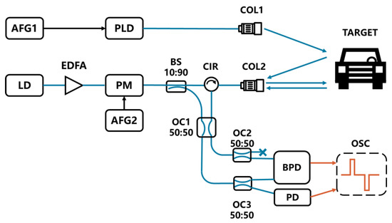
Figure 7.
A schematic of the experimental setup demonstrating the anti-interference capability against ToF. AFG: arbitrary function generator; PLD: pulsed laser; COL: collimator; LD: laser; EDFA: erbium-doped fiber amplifier; PM: phase modulator; OC: optical coupler; CIR: circulator; BPD: balance photodetector; PD: photodetector; and OSC: oscilloscope.
Figure 8a,b shows typical waveforms of the interfered RX signal and the IF signal, respectively. The pronounced peaking in Figure 8a indicates that the aggressor pulses have been received by the victim aperture and are concurrent with the PhMCW detection. As shown in Figure 8b, the aggressor pulse has negligible influence on the IF signal. The minor peaking in the IF signal, as circled in Figure 8b, is due to a minute imbalance resulting from the optical couplers or the balanced photodetectors.
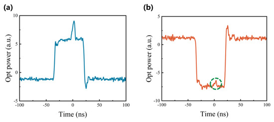
Figure 8.
Waveforms of the interfered RX signal (a) and IF signal (b).
We acquired 50 successive RX signals, as shown in Figure 9a. For better visibility, we only show every other four RX signals. It is obvious that the pulsed interference signals gradually advance in time with respect to the IF signals. This is because the AFGs are asynchronous and there is a minute frequency offset between them, even though their nominal frequencies are both 100 kHz. The pulse widths of the corresponding IF signals are obtained by the oscilloscope, and we can also conclude, from Figure 9a, that the timing relationship between the interference signal and the IF signal does not influence the ranging result. Figure 9b shows the ranging precision as a function of target distance with and without the interference signals. There is no significant difference between the two curves, suggesting the capability of anti-interference against ToF LiDARs. In order to reach a more quantitative conclusion, the Ljung–Box test is performed [34]. Briefly, if the interference has no influence on the PhMCW system, the difference of the measured precision with and without interference is thus a white noise, i.e., is Gaussian distributed random measurement error, where and are the measured precisions with and without interference, respectively. Subsequently, the Ljung–Box statistic is calculated using , where T = 6 is the sample size, m = 1 is the lag rank or degree of freedom, and is the n-order autocorrelation coefficient. Finally, the p-value is calculated by , where is the chi-square random variable. If the p-value is greater than 0.05, we cannot reject the null hypothesis that is white noise and thus interference does not influence the LiDAR system. The measured precision values are summarized in Table 1 and the p-value is calculated to be 0.0589, demonstrating the anti-interference capability against ToF LiDARs.
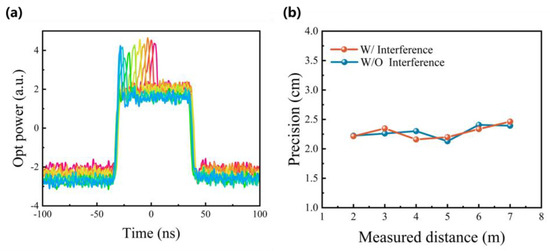
Figure 9.
(a) Superimposed image of the interfered RX signal. For better visibility, only 10 RX signals are shown. (b) Precision as a function of distance with and without interference.

Table 1.
Precision as a function of distance with and without ToF LiDAR interference.
For a commercial LiDAR, the echo waveform may not be measured during the anti-interference evaluation. To resolve this problem, we can first place the victim Lidar on an optical table and then observe the stationary scanning pattern by using an infrared camera. Subsequently, we can aim the interference source (AFG1 + PLD + COL1 in Figure 7) to a particular voxel and record the ranging results of the corresponding voxel as a function of time. The interference source can be amplitude-, frequency- or phase-modulated to mimic any possible interference in realistic applications. Finally, the Ljung–Box test is performed to quantitively determine the anti-interference capability, as mentioned above.
In addition to ToF, we also validated the immunity against coherent LiDARs. The diagram of the setup is illustrated in Figure 10. As a demonstration, the aggressor light source was another PhMCW laser operating at 1550 nm. The phase-modulation frequency of the aggressor laser was chosen to be 10 MHz, which is two orders of magnitude higher than that of the victim PhMCW system, guaranteeing that the phase-modulation interference was concurrent with the PhMCW detection. Prior to the anti-interference experiment, the aggressor laser was mechanically chopped and the waveform of the RX signal was monitored at either arm of the balanced detectors. Figure 11a shows the monitored RX signal and the negative rectangular pulse indicates that the aggressor light had been received by the victim aperture. Figure 11b shows the ranging precision as a function of distance with and without interference. The measured precision values are summarized in Table 2. The two curves exhibit negligible differences and the p-value is calculated to be 0.6327, illustrating the immunity against coherent LiDARs.
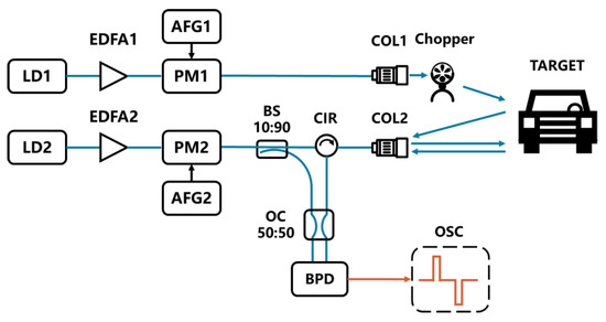
Figure 10.
A schematic of the experimental setup demonstrating anti-interference capability against coherent Lidars. LD: laser; EDFA: erbium-doped fiber amplifier; PM: phase modulator; AFG: arbitrary function generator; COL: collimator; OC: optical coupler; CIR: circulator; BPD: balance photodetector; and OSC: oscilloscope.
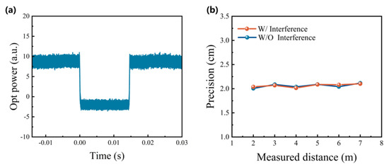
Figure 11.
(a) The optical waveform at either arm of the balanced photodetector. (b) Ranging precision as a function of distance with and without interference.
Table 2.
Precision as a function of distance with and without coherent Lidar interference.
5. Conclusions
This study demonstrated a phase-modulated continuous-wave (PhMCW) ranging method. Experimentally, we varied the distance of a diffusive reflection board to a furthest distance of 50 m, and a ranging error as low as 2.2 cm was achieved, which is comparable to that of commercial LiDARs. In addition, we modeled the ranging precision of the PhMCW system. Furthermore, a one-dimensional scanning LiDAR system that is capable of detecting targets at 28 m was built, demonstrating the validation of the PhMCW method. Subsequently, we proposed a quantitative method for evaluating the anti-interference capability of lidar systems. Specifically, the ranging precision was measured with and without interference, and the Ljung–Box test was performed to quantitatively illustrate the minimal influence of interference. The p-values were 0.0589 and 0.6327 with ToF and coherent LiDAR interferences, respectively, demonstrating that the PhMCW system is immune to interference. Additionally, the proposed method can be applied to all types of LiDAR systems, regardless of the ranging method or beam-steering technique used. To the best of our knowledge, this is the first quantitative method for evaluating the anti-interference capability of LiDARs.
The PhMCW ranging method is specifically suitable for applications with medium detection ranges such as autonomous vehicles, robotics, and drones. In Table 3, we have outlined the requirements for autonomous vehicle LiDAR and compared the performances of FMCW, commercial ToF, and the PhMCW methods. While the PhMCW has similar performances to commercial ToF LiDARs, it outperforms them with its excellent eye-safe feature and anti-interference ability. While FMCW has the best overall performance, it is limited by low stability, high complexity, and high insertion loss of the frequency-modulated source, as mentioned in references [7,32,35,36,37,38]. Thus, the PhMCW is a simple and effective ranging method that satisfies various applications such as autonomous vehicles, robotics, and drones.
Table 3.
Comparison among various LiDAR technologies.
Finally, it is worth noting that the PhMCW method is especially suitable for detection at 100 m, where the refractive index can be considered constant along the light trajectory. Although factors including temperature, pressure, and humidity inevitably lead to refractive index variation and result in ranging error, they can be calibrated in conjunction with temperature, pressure, and humidity sensors.
Author Contributions
Conceptualization, M.Z. and Y.W.; methodology, Y.W. and Q.H.; validation,M.Z., Y.W. and S.Z.; data curation, M.Z., L.L., Y.C.,Y.L., C.Q., P.J. and Y.S.; writing—original draft preparation, M.Z.; writing—review and editing, Y.W., L.L., Y.C., Y.L., C.Q., P.J. and Y.S.; project administration, Y.W., L.Q. and L.W. All authors have read and agreed to the published version of the manuscript.
Funding
This work was supported by the Science and Technology Development Project of Jilin Province (20230201033GX, 20200501006GX, 20200501007GX, 20200501008GX) and the National Natural Science Foundation of China (62090054).
Data Availability Statement
Data underlying the results presented in this paper are not publicly available at this time but may be obtained from the authors upon reasonable request.
Conflicts of Interest
The authors declare no conflict of interest.
References
- Zhang, X.; Kwon, K.; Henriksson, J.; Luo, J.; Wu, M.C. A large-scale microelectromechanical-systems-based silicon photonics LiDAR. Nature 2022, 603, 253–258. [Google Scholar] [CrossRef] [PubMed]
- Royo, S.; Ballesta-Garcia, M. An Overview of Lidar Imaging Systems for Autonomous Vehicles. Appl. Sci. 2019, 9, 4093. [Google Scholar] [CrossRef]
- Purdy, T. Bright squeezed light reduces back-action. Nat. Photonics 2019, 14, 1–2. [Google Scholar] [CrossRef]
- Sun, X.; Zhang, L.; Zhang, Q.; Zhang, W. Si Photonics for Practical LiDAR Solutions. Appl. Sci. 2019, 9, 4225. [Google Scholar] [CrossRef]
- Whyte, R.; Streeter, L.; Cree, M.J.; Dorrington, A.A. Application of lidar techniques to time-of-flight range imaging. Appl. Opt. 2015, 54, 9654–9664. [Google Scholar] [CrossRef]
- Bosch, T. Laser ranging: A critical review of usual techniques for distance measurement. Opt. Eng. 2001, 40, 10–19. [Google Scholar] [CrossRef]
- Rogers, C.; Piggott, A.Y.; Thomson, D.J.; Wiser, R.F.; Opris, I.E.; Fortune, S.A.; Compston, A.J.; Gondarenko, A.; Meng, F.; Chen, X.; et al. A universal 3D imaging sensor on a silicon photonics platform. Nature 2021, 590, 256–261. [Google Scholar] [CrossRef]
- Shi, J.W.; Guo, J.I.; Kagami, M.; Suni, P.; Ziemann, O. Photonic technologies for autonomous cars: Feature introduction. Opt. Express 2019, 27, 7627–7628. [Google Scholar] [CrossRef]
- Zhang, L.; Li, Y.; Chen, B.; Wang, Y.; Li, H.; Hou, Y.; Tao, M.; Li, Y.; Zhi, Z.; Liu, X.; et al. Two-dimensional multi-layered SiN-on-SOI optical phased array with wide-scanning and long-distance ranging. Opt. Express 2022, 30, 5008–5018. [Google Scholar] [CrossRef]
- Lee, S.-H.; Kwon, W.-H.; Lim, Y.-S.; Park, Y.-H. Highly precise AMCW time-of-flight scanning sensor based on parallel-phase demodulation. Measurement 2022, 203, 111860. [Google Scholar] [CrossRef]
- Byun, H.; Lee, J.; Jang, B.; Lee, C.; Ha, K. A gain-enhanced silicon-photonic optical phased array with integrated O-band amplifiers for 40-m ranging and 3D scan. In Proceedings of the 2020 Conference on Lasers and Electro-Optics (CLEO), San Jose, CA, USA, 10–15 May 2020. [Google Scholar]
- Behroozpour, B.; Sandborn, P.A.M.; Wu, M.C.; Boser, B.E. Lidar System Architectures and Circuits. IEEE Commun. Mag. 2017, 55, 135–142. [Google Scholar] [CrossRef]
- Taneski, F.; Abbas, T.A.; Henderson, R.K. Laser Power Efficiency of Partial Histogram Direct Time-of-Flight LiDAR Sensors. J. Light. Technol. 2022, 40, 5884–5893. [Google Scholar] [CrossRef]
- Lee, J.; Kim, Y.-J.; Lee, K.; Lee, S.; Kim, S.-W. Time-of-flight measurement with femtosecond light pulses. Nat. Photonics 2010, 4, 716–720. [Google Scholar] [CrossRef]
- Horaud, R.; Hansard, M.; Evangelidis, G.; Ménier, C. An overview of depth cameras and range scanners based on time-of-flight technologies. Mach. Vis. Appl. 2016, 27, 1005–1020. [Google Scholar] [CrossRef]
- Working with Lasers Updated to Include IEC. 2014. Available online: https://slideplayer.com/slide/12202834/ (accessed on 20 March 2023).
- Lum, D.J. Ultrafast time-of-flight 3D LiDAR. Nat. Photonics 2020, 14, 2–4. [Google Scholar] [CrossRef]
- Poulton, C.V.; Byrd, M.J.; Russo, P.; Timurdogan, E.; Khandaker, M.; Vermeulen, D.; Watts, M.R. Long-Range LiDAR and Free-Space Data Communication With High-Performance Optical Phased Arrays. IEEE J. Sel. Top. Quantum Electron. 2019, 25, 1–8. [Google Scholar] [CrossRef]
- Poulton, C.V.; Yaacobi, A.; Cole, D.B.; Byrd, M.J.; Raval, M.; Vermeulen, D.; Watts, M.R. Coherent solid-state LIDAR with silicon photonic optical phased arrays. Opt. Lett. 2017, 42, 4091–4094. [Google Scholar] [CrossRef]
- Zhang, T.; Qu, X.; Zhang, F. Nonlinear error correction for FMCW ladar by the amplitude modulation method. Opt. Express 2018, 26, 11519–11528. [Google Scholar] [CrossRef]
- Kamata, M.; Hinakura, Y.; Baba, T. Carrier-Suppressed Single Sideband Signal for FMCW LiDAR Using a Si Photonic-Crystal Optical Modulators. J. Light. Technol. 2020, 38, 2315–2321. [Google Scholar] [CrossRef]
- Shi, P.; Lu, L.; Liu, C.; Zhou, G.; Xu, W.; Chen, J.; Zhou, L. Optical FMCW Signal Generation Using a Silicon Dual-Parallel Mach-Zehnder Modulator. IEEE Photonics Technol. Lett. 2021, 33, 301–304. [Google Scholar] [CrossRef]
- Kittlaus, E.A.; Eliyahu, D.; Ganji, S.; Williams, S.; Matsko, A.B.; Cooper, K.B.; Forouhar, S. A low-noise photonic heterodyne synthesizer and its application to millimeter-wave radar. Nat. Commun. 2021, 12, 4397. [Google Scholar] [CrossRef] [PubMed]
- Zhang, X.; Pouls, J.; Wu, M.C. Laser frequency sweep linearization by iterative learning pre-distortion for FMCW LiDAR. Opt. Express 2019, 27, 9965–9974. [Google Scholar] [CrossRef] [PubMed]
- Popko, G.B.; Gaylord, T.K.; Valenta, C.R. Interference measurements between single-beam, mechanical scanning, time-of-flight lidars. Opt. Eng. 2020, 59, 053106. [Google Scholar] [CrossRef]
- Hwang, I.-P.; Lee, C.-H. Mutual Interferences of a True-Random LiDAR With Other LiDAR Signals. IEEE Access. 2020, 8, 124123–124133. [Google Scholar] [CrossRef]
- Grollius, S.; Buchner, A.; Ligges, M.; Grabmaier, A. Probability of Unrecognized LiDAR Interference for TCSPC LiDAR. IEEE Sens. J. 2022, 22, 12976–12986. [Google Scholar] [CrossRef]
- Lee, B.-C.; Choi, B.-C.; Bang, H.-S.; Koh, Y.N.; Han, K.-Y. Study on Measurement Error Reduction Using the Internal Interference Light Reduction Structure of a Time-of-Flight Sensor. IEEE Sens. J. 2022, 22, 12967–12975. [Google Scholar] [CrossRef]
- Dashpute, A.; Anand, C.; Sarkar, M. Depth Resolution Enhancement in Time-of-Flight Cameras Using Polarization State of the Reflected Light. IEEE Trans. Instrum. Meas. 2019, 68, 160–168. [Google Scholar] [CrossRef]
- Jiménez, D.; Pizarro, D.; Mazo, M.; Palazuelos, S. Modeling and correction of multipath interference in time of flight cameras. Image Vis. Comput. 2014, 32, 1–13. [Google Scholar] [CrossRef]
- Popko, G.B.; Gaylord, T.K.; Valenta, C.R.; Turner, M.D.; Kamerman, G.W. Signal interactions between lidar scanners. In Laser Radar Technology and Applications XXIV; SPIE: Bellingham, WA, USA, 2019. [Google Scholar]
- Carballo, A.; Lambert, J.; Monrroy-Cano, A.; Wong, D.R.; Narksri, P.; Kitsukawa, Y.; Takeuchi, E.; Kato, S.; Takeda, K. LIBRE: The Multiple 3D LiDAR Dataset. In Proceedings of the 2020 IEEE Intelligent Vehicles Symposium (IV), Las Vegas, NV, USA, 19 October–13 November 2020. [Google Scholar]
- Thurn, K.; Ebelt, R.; Vossiek, M. Noise in Homodyne FMCW radar systems and its effects on ranging precision. In Proceedings of the 2013 IEEE MTT-S International Microwave Symposium Digest (MTT), Seattle, WA, USA, 2–7 June 2013. [Google Scholar]
- Ljung, G.M.; Box, G.E. On a Measure of Lack of Fit in Time Series Models. Biometrika 1978, 65, 297–303. [Google Scholar] [CrossRef]
- Li, Y.; Chen, B.; Na, Q.; Xie, Q.; Tao, M.; Zhang, L.; Zhi, Z.; Li, Y.; Liu, X.; Luo, X.; et al. Wide-steering-angle high-resolution optical phased array. Photonics Res. 2021, 9, 2511–2518. [Google Scholar] [CrossRef]
- Poulton, C.V.; Byrd, M.J.; Russo, P.; Moss, B.; Shatrovoy, O.; Khandaker, M.; Watts, M.R. Coherent LiDAR With an 8,192-Element Optical Phased Array and Driving Laser. IEEE J. Sel. Top. Quantum Electron. 2022, 28, 1–8. [Google Scholar] [CrossRef]
- Velodyne. Velodyne. Available online: https://velodynelidar.com/ (accessed on 20 March 2023).
- Robosense. Robosense. Available online: https://www.robosense.cn/ (accessed on 20 March 2023).


Disclaimer/Publisher’s Note: The statements, opinions and data contained in all publications are solely those of the individual author(s) and contributor(s) and not of MDPI and/or the editor(s). MDPI and/or the editor(s) disclaim responsibility for any injury to people or property resulting from any ideas, methods, instructions or products referred to in the content. |
© 2023 by the authors. Licensee MDPI, Basel, Switzerland. This article is an open access article distributed under the terms and conditions of the Creative Commons Attribution (CC BY) license (https://creativecommons.org/licenses/by/4.0/).