3.1. Materials
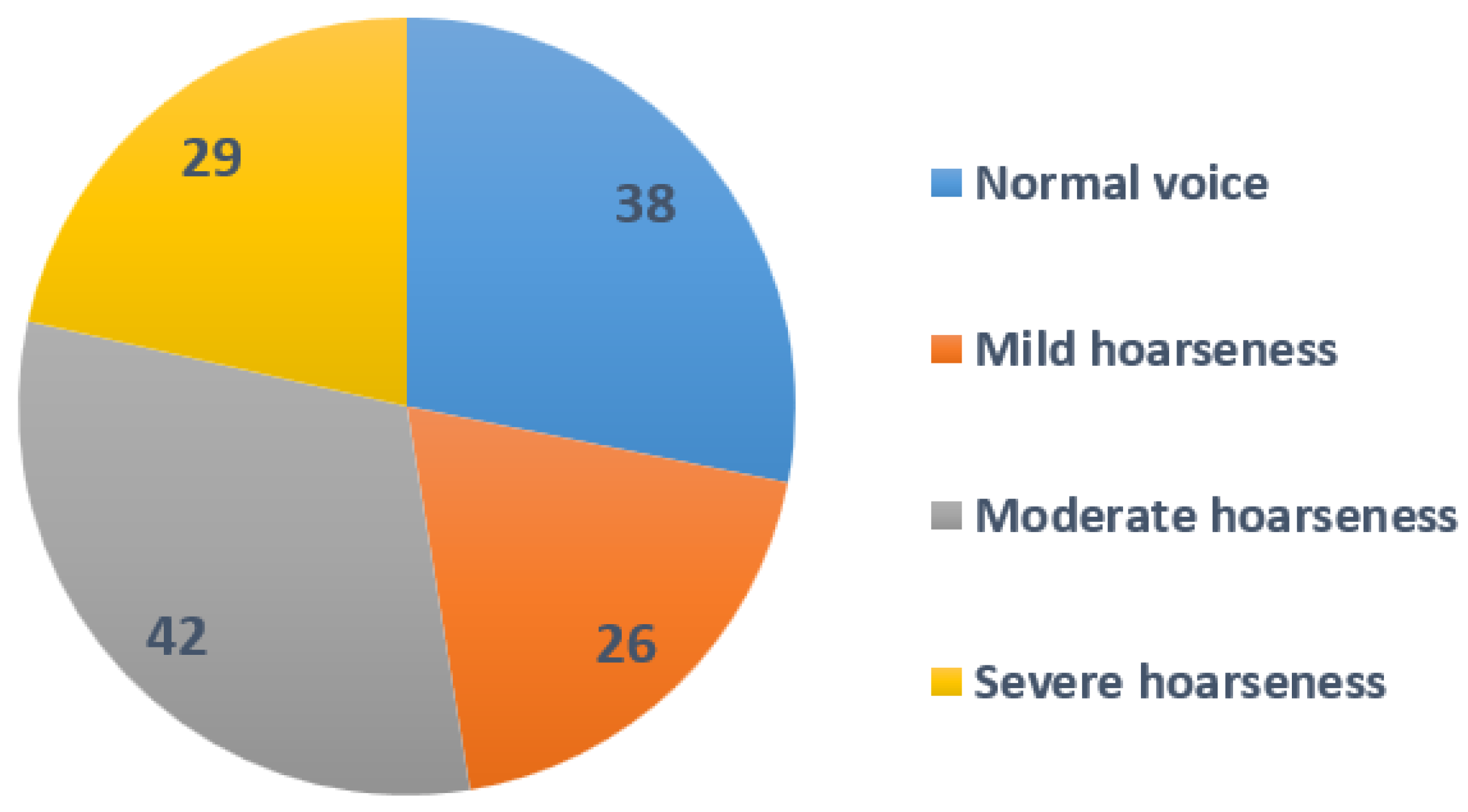
The study comprised 134 adult participants, with 58 men and 77 women, who were evaluated in the Department of Otolaryngology of the Lithuanian University of Health Sciences, Kaunas, Lithuania. The mean age of the participants was 42.9 (SD 15.26) years. The pathological voice subgroup, which included 86 patients (42 men and 44 women), had a mean age of 50.8 years (SD 14.3) and presented with a variety of laryngeal diseases and associated voice impairments, such as benign and malignant mass lesions of the vocal folds and unilateral paralysis of the vocal fold. Diagnosis was based on clinical examination, including patient complaints and history, voice assessment and video laryngostroboscopy (VLS) using an XION Endo-STROB DX device (XION GmbH, Berlin, Germany) 70° rigid endoscope and/or direct microlaryngoscopy. Five experienced physicians–laryngologists performed the auditory–perceptual evaluations of voice samples. For the purpose of this study, only the evaluation of dysphonia’s grade (G) was used from the GRBAS scale (grade, breathiness, roughness, asthenia, and strain). The voice samples were rated into four ordinal severity classes of G on the scale from 0 to 3 points, where 0 = normal voice, 1—mild, 2—moderate, and 3—severe dysphonia [
64]. A severity distribution is displayed in
Figure 1.
The normal voice subgroup consisted of 49 healthy volunteers, 16 men and 33 women, with a mean age of 31.69 (SD 9.89) years. To qualify as vocally healthy, participants were required to have no actual voice complaints, no history of chronic laryngeal diseases or voice disorders, and to self-report their voice as normal. The voices of the participants were evaluated as normal by otolaryngologists specialized in the field of voice, as there were no pathological alterations in the larynx. Demographic data for the study group and diagnoses for the pathological voice subgroup are presented in
Table 1.
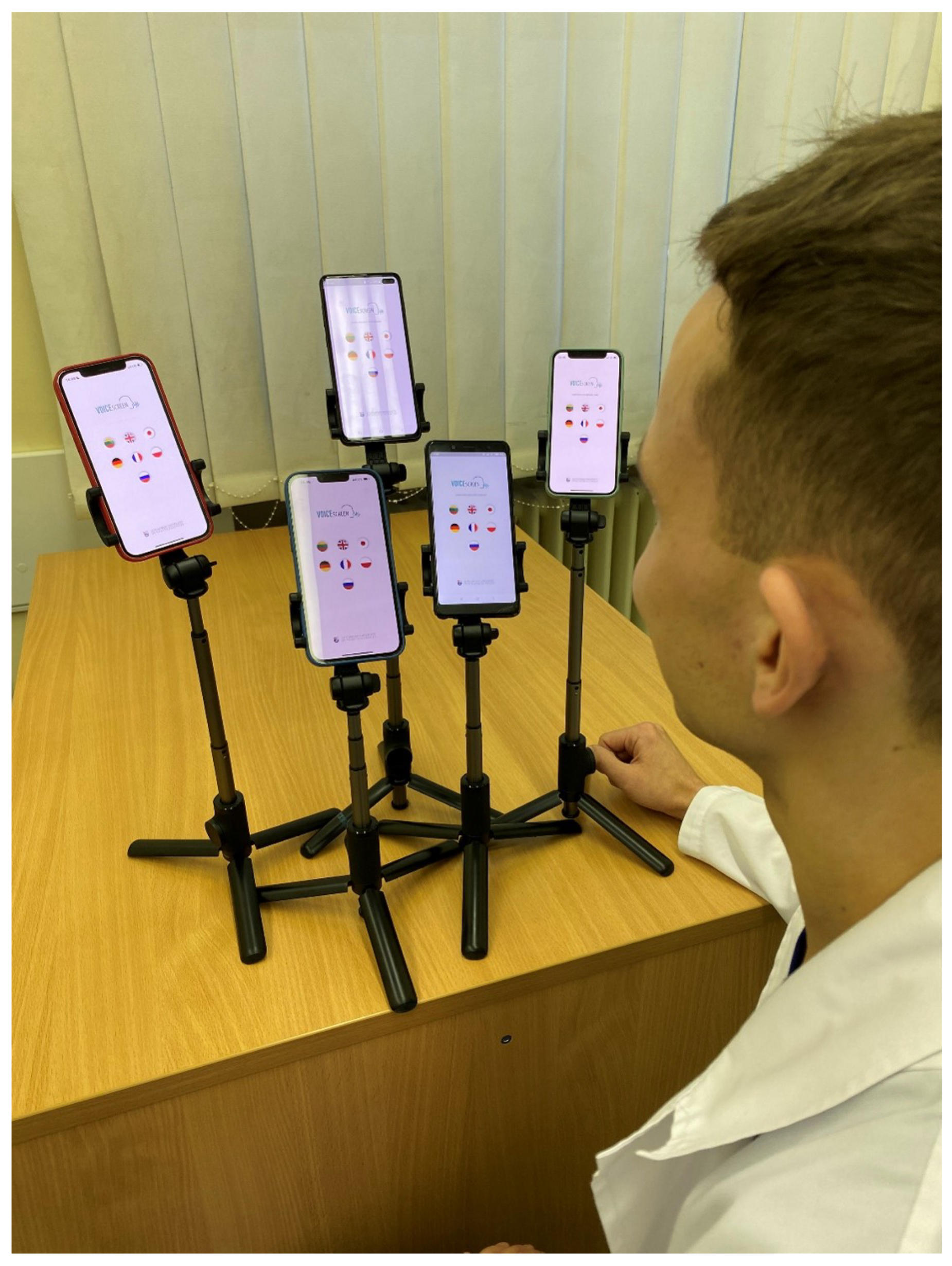
Voice samples representing five different smartphones were used, namely the iPhone 12 Pro, iPhone 13 Pro Max, Xiaomi Redmi Note 5, iPhone 12 Mini, and Samsung Galaxy S10+. The following processing conditions were applied: smartphones were placed approximately 30.0 cm away from the mouth, at a 90
angle to the mouth, and had internal microphones (bottom) (see
Figure 2). The devices were selected from a range of commercial prices. The background noise level averaged 29.61 dB SPL and the signal-to-noise ratio (SNR) was approximately 38.11 dB compared to the voiced recordings, indicating that the environment was suitable for both voice recordings and the extraction of acoustic parameters. The AKG microphone was placed 10.0 cm from the mouth at a comfortable (approximately 90°) microphone-to-mouth angle.
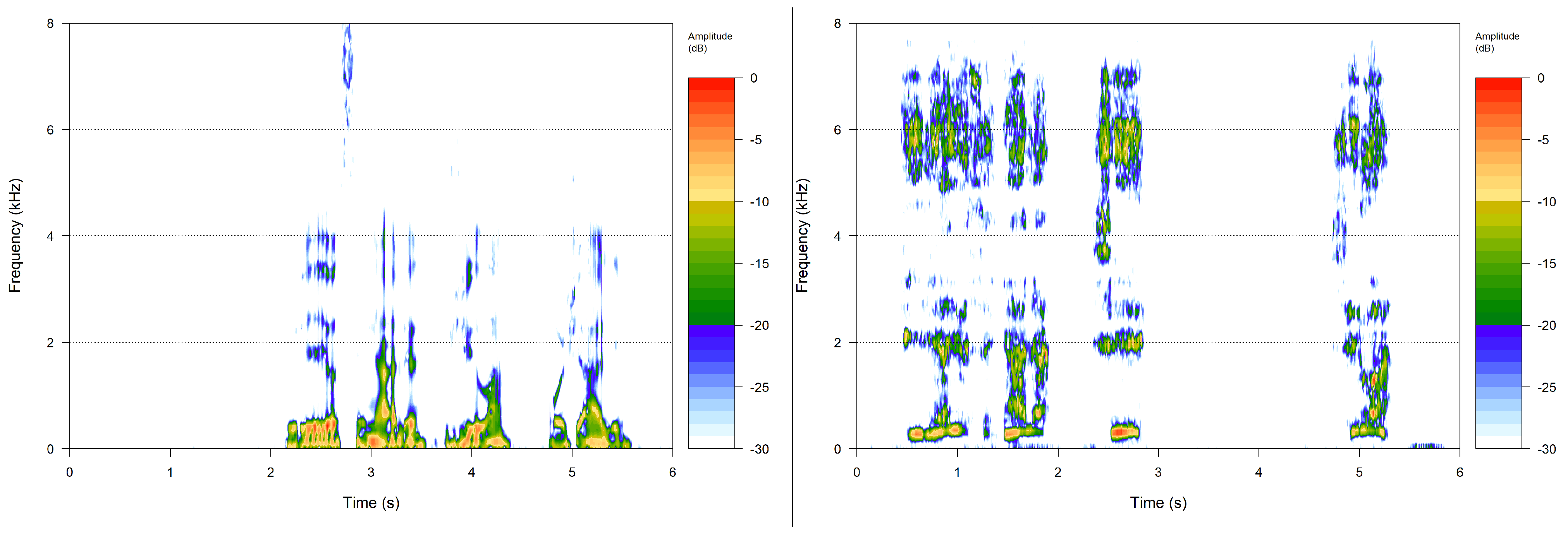
A phonetically balanced Lithuanian sentence “Turėjo senelė žilą oželį” (“Old granny had a billy goat”) was the main utterance used to compare the recordings. The relative frequencies of the phonemes in the sentence are as close as possible to the distribution of speech sounds used in Lithuanian. The examples of spectral analysis results of voice samples are given in
Figure 3.
3.2. Calculating Required Voice Characteristics
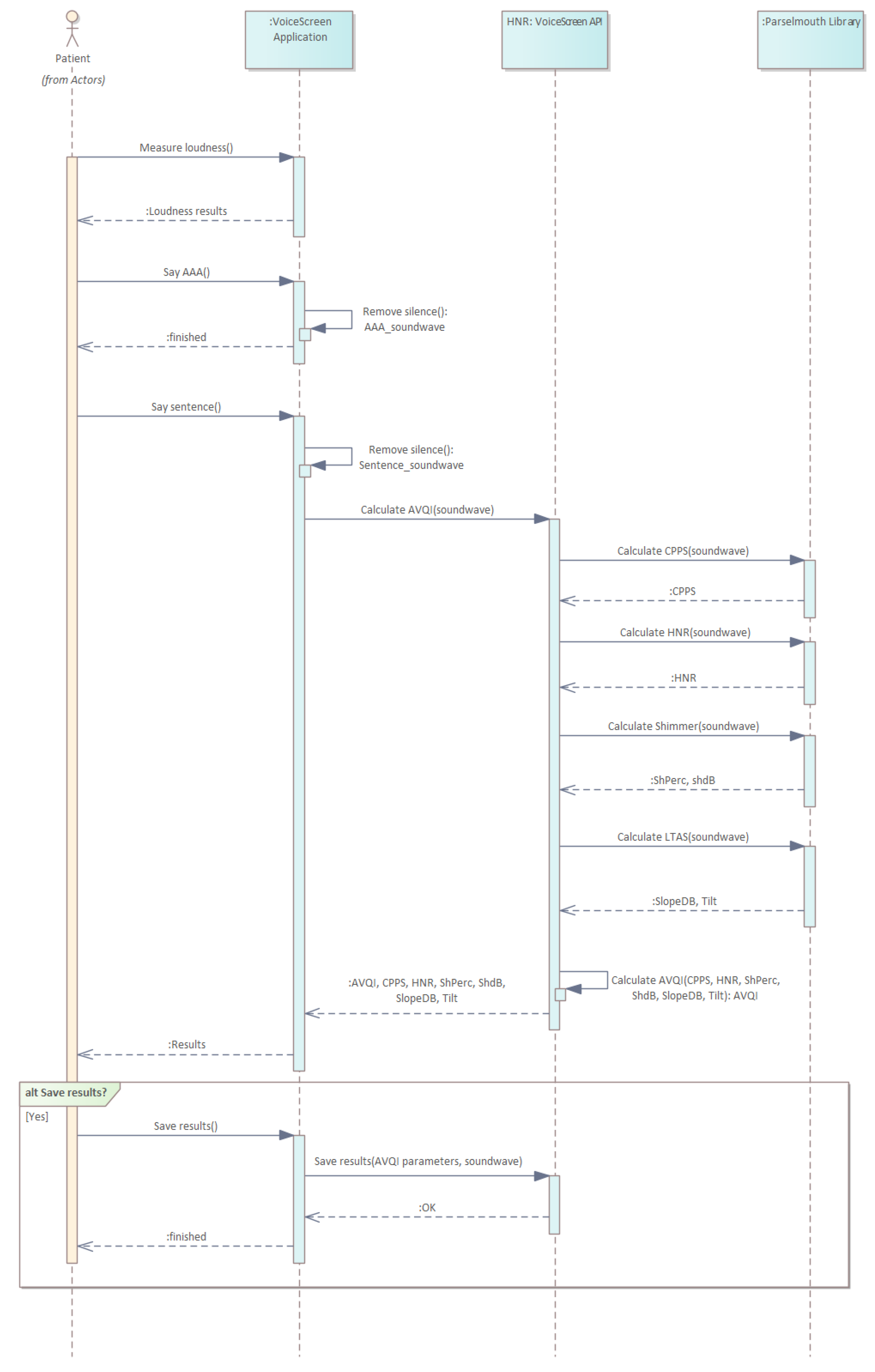
To conduct the clinical research, we built a universal-platform-based version of the “VoiceScreen” software for use with both iOS and Android operating systems, using our Pareto optimized technique. The AVQI and its characteristics are calculated on the server; hence, computationally expensive sound processing is not reliant on the computing capabilities of the user device and may run on any Android or iOS device with a manufacturer-supported version of each respective operating system. The provided smartphone (either iOS or Android) records sound waves obtained while pronouncing given sentences aloud in the first stage. Sound waves are preprocessed in real time. The goal is to remove pauses from the sound waves and to guarantee that only the minimum quantity of sound is available for further processing. Then, that preprocessed sound wave is sent to the server for further analysis. The server runs a Linux operating system and operates our proprietary software to calculate the required characteristics necessary to evaluate the voice. Finally, the AVQI index and related data are sent back to the phone and displayed to the user.
Figure 4 shows the structure of the system, while
Figure 5 illustrates the operation sequence.
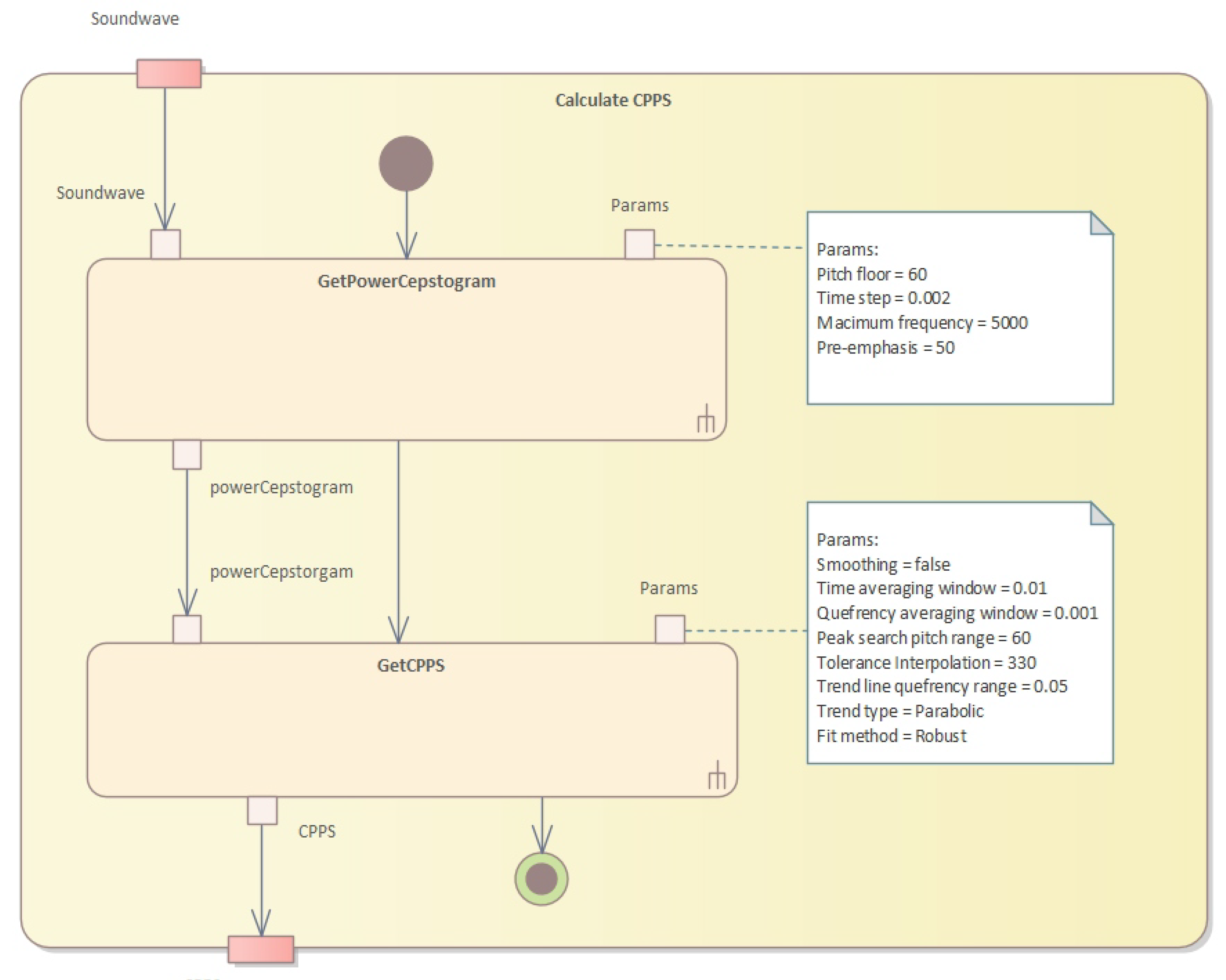
The server-side system performs numerous operations. First, the cepstral peak prominence (CPPS) is calculated (see
Figure 6).
Our approach outlines a series of algorithms used to assess impaired voice quality using acoustic measures. The first algorithm resamples and applies pre-emphasis to the sound, then calculates the power cepstrogram. The second algorithm calculates the harmonicity using the cross-correlation technique, while the third algorithm calculates the shimmer, which measures cycle-to-cycle variations in vocal amplitude. The fourth algorithm calculates the long-term average spectrum (LTAS) of the sound waveform. Finally, the AVQI values are calculated, using multiple acoustic measures of voice quality through Pareto optimization. This technique identifies the optimal trade-off between multiple conflicting objectives to find the best solution to improve overall vocal quality while minimizing breathiness, roughness, and strain.
In Algorithm 1, we first resample the sound to twice the value of the maximum frequency and apply pre-emphasis to the resampled sound. Then, for each analysis window, we apply a Gaussian window, calculate the spectrum, transform it into a PowerCepstrum and store the values in the corresponding vertical slice of the PowerCepstrogram matrix. The algorithm returns the resulting PowerCepstrogram. The PowerCepstrogram is a representation of the power spectrum of a signal in the cepstral domain. The algorithm takes as input a sound signal, a pitch floor, a time step, a maximum frequency, and a pre-emphasis coefficient. The output of the algorithm is the PowerCepstrogram.
| Algorithm 1 PowerCepstogram algorithm. |
Require:
Ensure: PowerCepstrogram
- 1:
function PowerCepstrogram() - 2:
Resample() - 3:
Pre-emphasize() - 4:
- 5:
Gaussian window with length - 6:
length of - 7:
- 8:
- 9:
empty matrix with dimensions - 10:
for to do - 11:
- 12:
- 13:
- 14:
Spectrum() - 15:
- 16:
PowerCepstrum() - 17:
values from up to - 18:
end for - 19:
return - 20:
end function
|
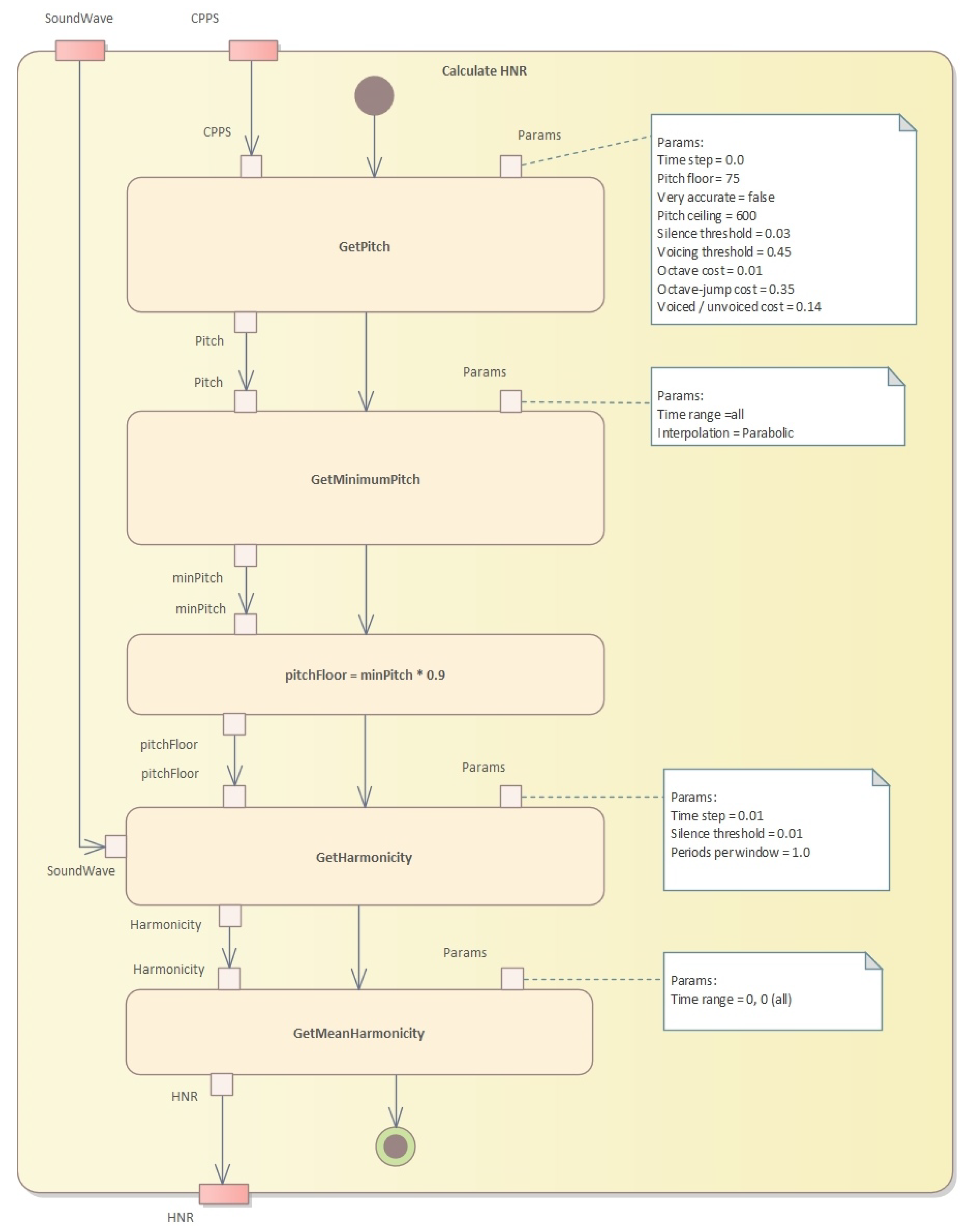
The second step is to perform pitch analysis and calculate harmonicity (see
Figure 7 and Algorithm 2).
Algorithm 2 shows an implementation of the pitch analysis method that uses the cross-correlation technique to determine the pitch of a sound signal. The input parameters are the sound signal, the time step, the pitch floor and ceiling, as well as various thresholds and costs that affect the pitch analysis. The algorithm returns a pitch object that contains the pitch measurements and other pitch-related information.
The formant calculation algorithm is presented in Algorithm 3. This algorithm is a partial implementation of a function called “getFormantMean” that calculates the average value of a specified formant for a given time range. The function takes four arguments: “formantNum” specifies which formant to calculate the mean for, “fromTime” and “toTime” specify the time range to consider, and “units” specifies the units of the time range.
Algorithm 4 presents an algorithm to calculate harmonicity using Praat’s harmonicity object. This algorithm takes a Praat sound object, a start and end time for the analysis, a time step, a silence threshold, and the number of periods per analysis window. It first creates a Praat harmonicity object from the input sound, with the given time step, silence threshold, and periods per window. It then selects the portion of the harmonicity object corresponding to the specified time range and returns the mean value of the selected portion. Aproach is explained in the Algorithm 4.
| Algorithm 2 Pitch analysis based on the cross-correlation method. |
- 1:
function PitchAnalysis() - 2:
Resample(, ) - 3:
PreEmphasize(, ) - 4:
- 5:
if then - 6:
- 7:
end if - 8:
if then - 9:
- 10:
end if - 11:
CreateEmptyPitch() - 12:
SetTimeStep(, ) - 13:
SetPitchFloor(, ) - 14:
SetSilenceThreshold(, ) - 15:
SetVoicingThreshold(, ) - 16:
SetCeiling(, ) - 17:
SetOctaveCost(, ) - 18:
SetOctaveJumpCost(, ) - 19:
SetVoicedUnvoicedCost(, ) - 20:
for in with interval of do - 21:
the length of the analysis window - 22:
CreateWindow(, ) - 23:
Autocorrelate() - 24:
ExtractCandidates(, , ) - 25:
FindBestCandidate(, ) - 26:
AddPitchMeasurement(, , ) - 27:
end for - 28:
PostProcessPitch() - 29:
return - 30:
end function
|
| Algorithm 3 Formant calculation. |
- 1:
function getFormantMean() - 2:
selected Formant object - 3:
- 4:
- 5:
for to n do - 6:
time at index i of formantObj - 7:
if or then - 8:
continue - 9:
end if - 10:
end for - 11:
formant value at index i, formant number of formantObj - 12:
end function
|
| Algorithm 4 Harmonicity calculation. |
- 1:
function CalculateHarmonicity() - 2:
ToHarmonicity(, , , ) - 3:
Select(harmonicity, , ) - 4:
return Get_mean(harmonicity) - 5:
end function
|
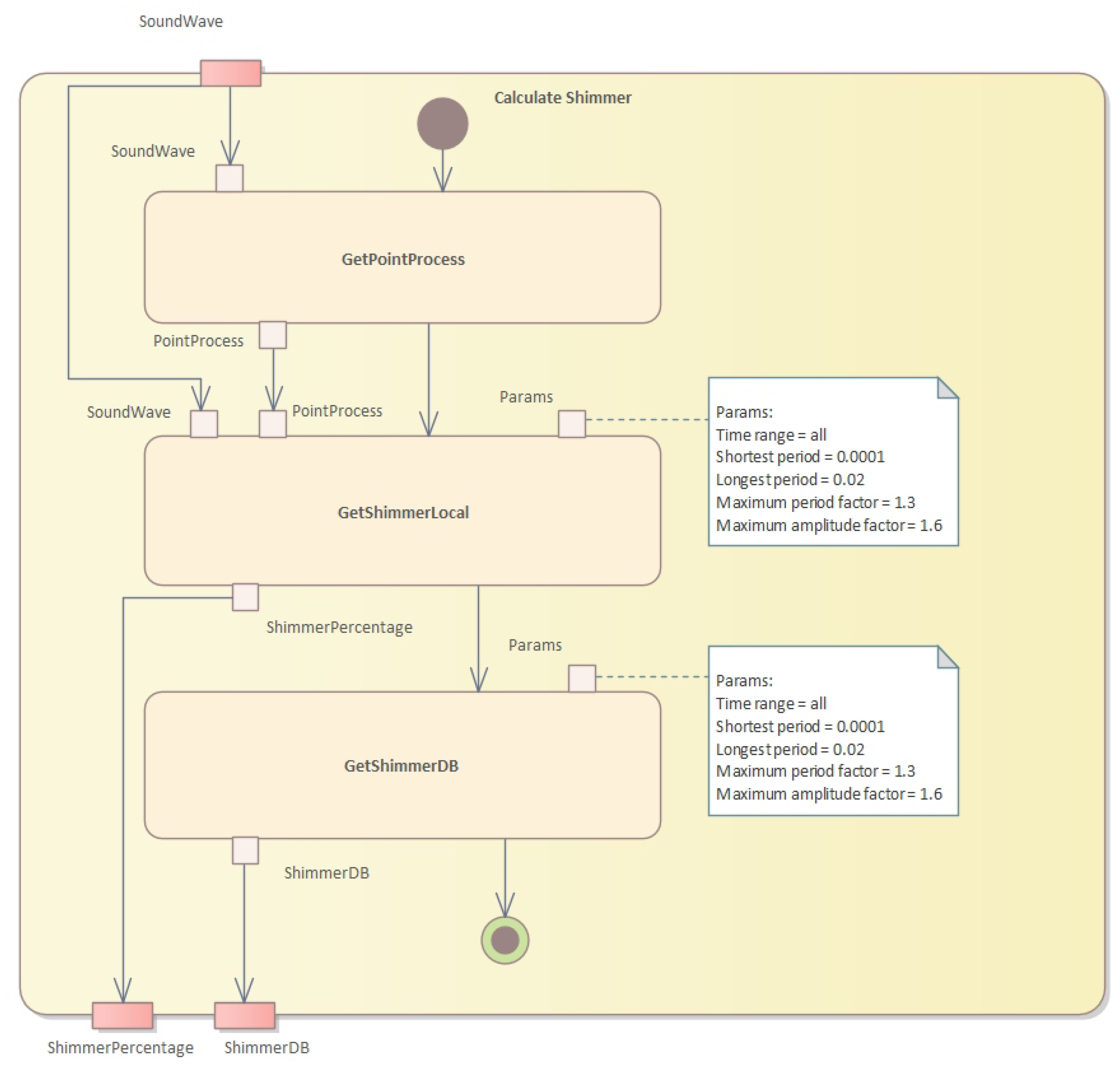
The third step is to calculate the shimmer (see
Figure 8 and Algorithm 5).
This algorithm calculates two measures of shimmer, which is a measure of cycle-to-cycle variations in vocal amplitude. The input is a sound waveform, a point process representing glottal closures, and the start and end times in seconds. The output is the shimmer local value and the shimmer dB value.
| Algorithm 5 Shimmer calculation. |
Require: , the sound waveform
Require: , the point process representing glottal closures
Require: , the start time in seconds
Require: , the end time in seconds
Ensure: , the shimmer local value
Ensure: , the shimmer dB value
- 1:
Extract a pitch contour from the sound using the Sound: To Pitch… command with the following settings: - 2:
- pitch floor: 75 Hz - 3:
- pitch ceiling: 600 Hz - 4:
- time step: 0.01 s - 5:
- range of analysis: to - 6:
Convert the pitch contour to a point process using the Pitch: To PointProcess command with the following settings: - 7:
- silences: unvoiced - 8:
- voicing threshold: 0.45 - 9:
Initialize a list to store the amplitude differences - 10:
for each period in the point process do - 11:
Get the start and end times of the period - 12:
Calculate the amplitude difference between the two points in the waveform that correspond to the start and end times - 13:
Append the absolute value of the amplitude difference to the list - 14:
end for - 15:
Calculate the average amplitude difference and the average amplitude: - 16:
- Calculate the mean of the amplitude difference list and store it as - 17:
- Calculate the mean of the absolute values of the waveform and store it as - 18:
Calculate the shimmer local value: - 19:
- Divide by and multiply by 100 - 20:
- Store the result as - 21:
Calculate the shimmer dB value: - 22:
- Calculate the base-10 logarithm of each amplitude difference value in the list and store the result as a new list - 23:
- Calculate the mean of the new list and multiply by 20 - 24:
- Store the result as - 25:
Return and
|
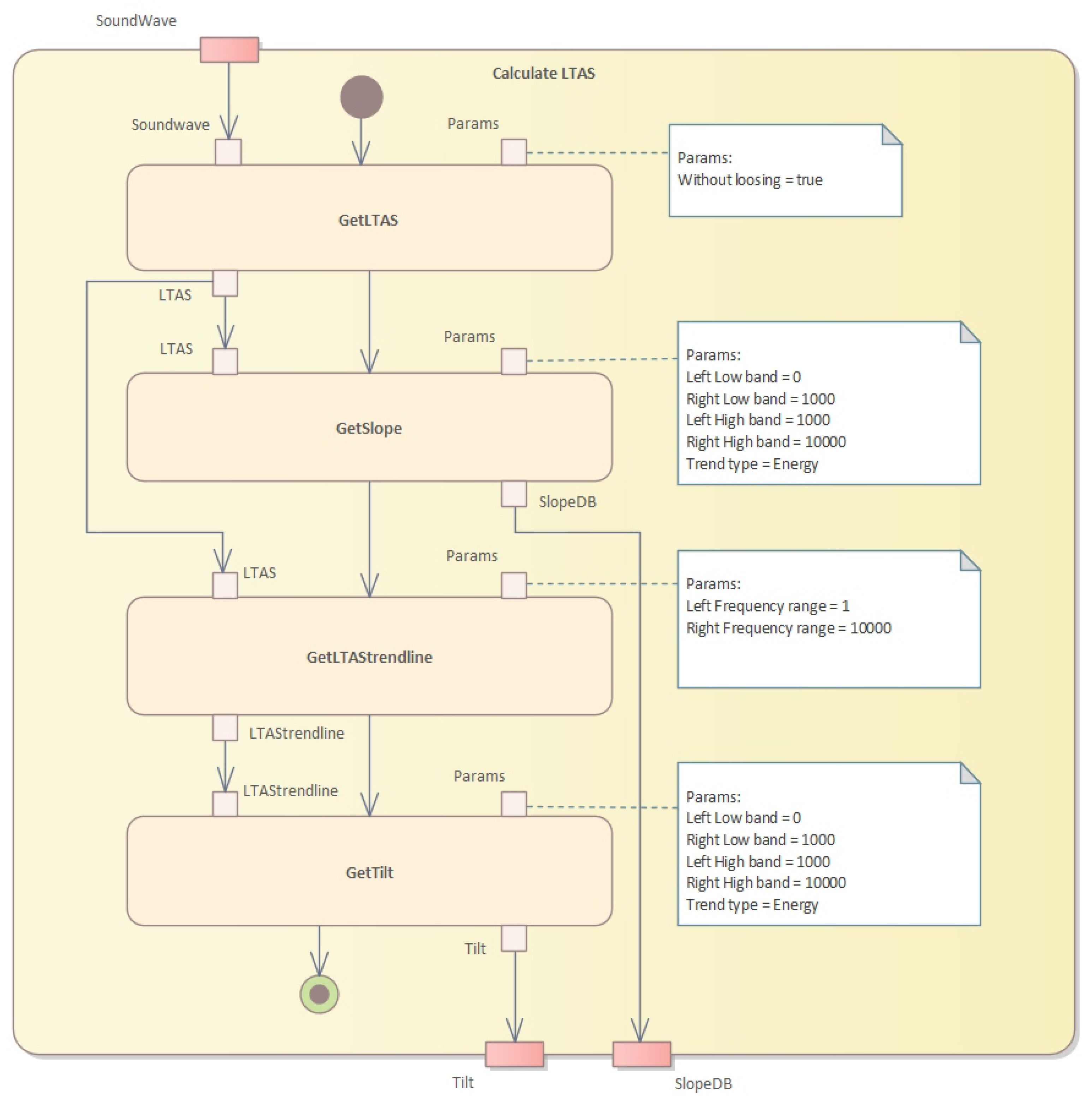
In the fourth step, we need to calculate the long-term average spectrum (LTAS) (see
Figure 9).
The algorithm to calculate the LTAS (long-term average spectrum) is presented in Algorithm 6. This algorithm calculates the LTAS of a given sound waveform and computes the slope and tilt parameters. The LTAS is a smoothed version of the spectrum of the sound waveform, calculated over a long period of time, typically several seconds.
| Algorithm 6 LTAS calculation. |
Require: : the sound waveform
Ensure: : the slope in dB and : the tilt parameter
- 1:
call(soundWav, “To Ltas…”, 1) ▹ Convert sound waveform to Ltas - 2:
for to do ▹ Calculate power in each band - 3:
call(ltas, “Get frequency”, i) - 4:
call(ltas, “Get real”, i) - 5:
call(ltas, “Get imaginary”, i) - 6:
▹ Calculate band power - 7:
end for - 8:
call(ltas, “Get slope…”, 0, 1000, 1000, 10000, “energy”) ▹ Calculate slope - 9:
call(ltas, “Compute trend line”, 1, 10000) ▹ Compute trendline - 10:
call(ltas_trendline_db, “Get slope”, 0, 1000, 1000, 10000, “energy”) ▹ Calculate tilt parameter - 11:
return ,
|
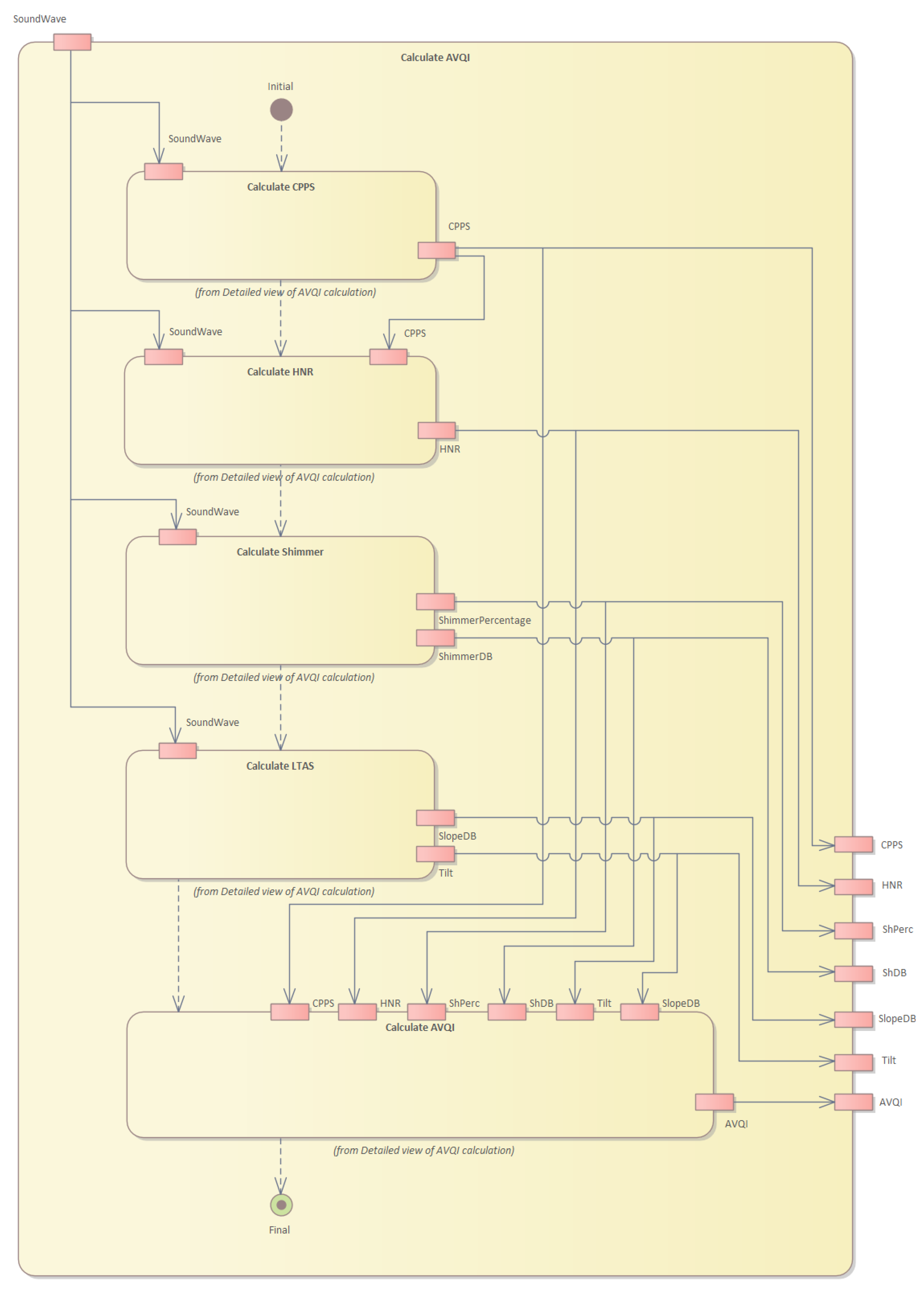
Finally, we calculate the AVQI values (see
Figure 10) given several acoustic measures of voice quality. The calculation algorithm is given in Algorithm 7. The Pareto optimization of AVQI scores is given in Algorithm 8.
| Algorithm 7 AVQI calculation. |
Require:
Ensure: AVQI
- 1:
function CalculateAVQI() - 2:
- 3:
return - 4:
end function
|
| Algorithm 8 Pareto optimization of AVQI scores. |
- 1:
Define the relevant voice quality parameters and define AVQI score as the objective to be optimized. - 2:
Select a set of candidate solutions that represent different combinations of the voice quality parameters. - 3:
Calculate the AVQI scores for each candidate solution using a combination of objective and subjective methods. - 4:
Plot the candidate solutions on a Pareto front to visualize the trade-off between the objectives. - 5:
Identify the Pareto optimal solutions on the Pareto front using visual inspection, clustering, or optimization algorithms, such as NSGA-II. - 6:
Select the Pareto optimal solution that best meets the specific needs and preferences of the AVQI assessment, considering factors such as clinical relevance, patient preference, and ease of implementation. - 7:
Evaluate the performance of the AVQI algorithm using validation data and feedback from clinicians and patients. - 8:
Fine-tune the AVQI algorithm and the Pareto optimization parameters based on the validation results and feedback.
|
Pareto Optimized Assessment of Impaired Voice
Pareto optimization is a technique used to identify the optimal trade-off between multiple conflicting objectives.
Let X be the set of candidate solutions, where each solution is a vector of n characteristics of voice quality, such as overall voice quality, strain, and pitch. Let be a vector of m objective functions that measure the performance of x in each characteristic. The Pareto front is defined as the set of nondominated solutions, i.e., those solutions that cannot be improved in any objective without worsening at least one other objective. Formally, a solution dominates another solution if and only if , and and there exists at least one objective function such that . The Pareto front is the set of all non-dominated solutions, i.e., is not dominated by . The Pareto optimal solution is any solution that maximizes the trade-off between the objectives, i.e., , where ≤ denotes Pareto dominance.
In the context of the evaluation of impaired voice by AVQI recorded on the smartphone, Pareto optimization is used to find the best trade-off between different parameters that affect overall vocal quality, such as breathiness, roughness, strain, and pitch. The first step in Pareto optimization is to define the objectives or criteria that need to be optimized. In the case of the AVQI assessment, the objective could be to maximize overall vocal quality while minimizing breathiness, roughness, and strain. Pitch could be considered a separate objective, depending on the specific voice impairment being assessed. The next step is to generate a set of candidate solutions that represent different combinations of objectives. This is done by varying the weights or importance assigned to each objective in the AVQI algorithm. For example, increasing the weight of the overall vocal quality objective would result in a higher score for samples with better overall quality, while decreasing the weight of the breathiness objective would result in a lower score for samples with more breathiness. Once the candidate solutions are generated, Pareto optimization techniques are used to identify the optimal trade-off between the objectives as follows.
Step 1: Calculate the AVQI scores for each candidate solution based on the relevant parameters.
To calculate the AVQI score, we need to first define the relevant parameters that affect voice quality. These could include measures of pitch, loudness, jitter, shimmer, harmonics-to-noise ratio, and other relevant acoustic and perceptual measures. Once the parameters are defined, we can use a combination of objective and subjective methods to calculate the AVQI score. Objective methods use signal processing and machine learning techniques to analyze the acoustic properties of the voice signal and extract relevant features. These features are then combined using a mathematical model to calculate the AVQI score. Examples of objective methods include Praat software, which measures various voice parameters, and the glottal inverse filtering (GIF) method, which estimates the glottal source waveform from the speech signal. Subjective methods use human listeners to rate the quality of the voice based on perceptual criteria, such as clarity, naturalness, and overall acceptability. These ratings are then combined using statistical methods to calculate the AVQI score. Examples of subjective methods include the consensus auditory–perceptual evaluation of voice (CAPE-V), which uses a standardized rating scale to evaluate various aspects of voice quality.
Step 2: Plot the candidate solutions on a Pareto front to visualize the trade-off between the objectives.
To plot the candidate solutions on a Pareto front, we first need to define the objective functions that we want to optimize. For example, we may want to maximize the clarity of the voice while minimizing the jitter and shimmer. We can then calculate the objective values for each candidate solution and plot them on a 2D or 3D graph, where each axis represents an objective function. The Pareto front is the set of candidate solutions that cannot be improved in one objective without sacrificing another objective.
Step 3: Identify the Pareto optimal solutions on the Pareto front that cannot be improved in one objective without sacrificing another objective.
To identify the Pareto optimal solutions, we can use a variety of techniques, such as visual inspection, clustering, or optimization algorithms. Visual inspection involves manually examining the Pareto front and selecting the solutions that best meet the specific needs and preferences of the AVQI assessment. Clustering involves grouping similar solutions together and selecting the representative solutions from each cluster. Optimization algorithms, such as the NSGA-II (non-dominated sorting genetic Algorithm 2) can be used to automatically identify the Pareto optimal solutions.
Step 4: Select the Pareto optimal solution that best meets the specific needs and preferences of the AVQI assessment.
To select the Pareto optimal solution that best meets the specific needs and preferences of the AVQI assessment, we need to consider factors, such as clinical relevance, patient preference, and ease of implementation. We may also want to consult with clinicians and patients to get their feedback and ensure that the selected solution is acceptable and feasible.
Step 5: Fine-tune the AVQI algorithm and the Pareto optimization parameters based on the validation results and feedback from clinicians and patients
To fine-tune the AVQI algorithm and the Pareto optimization parameters, we need to evaluate the performance of the algorithm using validation data and feedback from clinicians and patients. We can use metrics such as accuracy, sensitivity, specificity, and AUC (area under the roc curve) to assess the performance of the AVQI algorithm. We can also ask clinicians and patients to rate the quality of the voice for a subset of the validation data and compare the ratings with the AVQI scores. Based on the validation results and feedback.


 ,
, 


